Figure 1.
Calculation of the output by applying a convolution filter to an input layer represented by the matrix.
Figure 1.
Calculation of the output by applying a convolution filter to an input layer represented by the matrix.
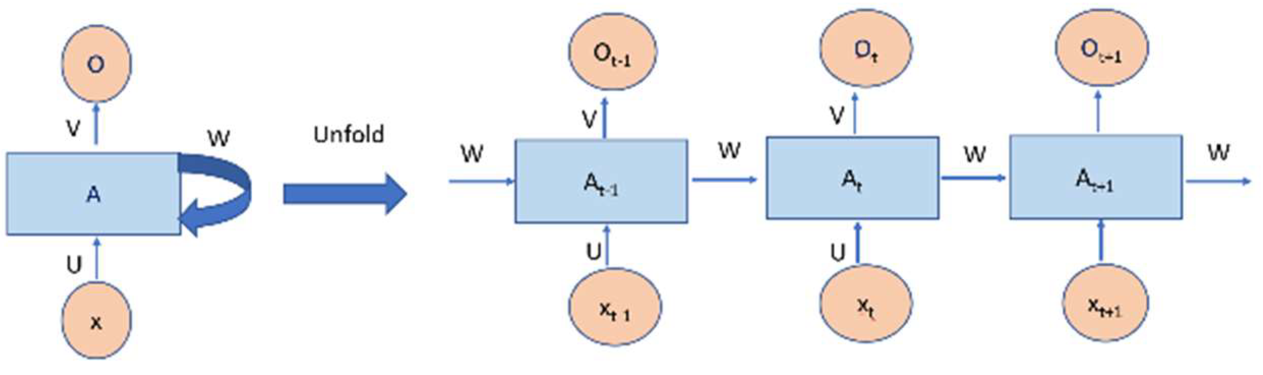
Figure 2.
An unrolled recurrent neural network.
Figure 2.
An unrolled recurrent neural network.
Figure 3.
One memory cell of a long short-term memory network.
Figure 3.
One memory cell of a long short-term memory network.
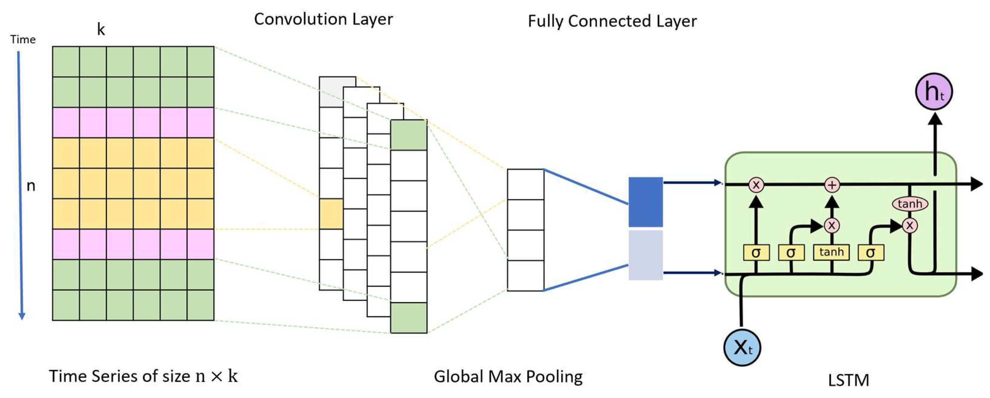
Figure 4.
The proposed hybrid model.
Figure 4.
The proposed hybrid model.
Figure 5.
The vector output LSTM model.
Figure 5.
The vector output LSTM model.
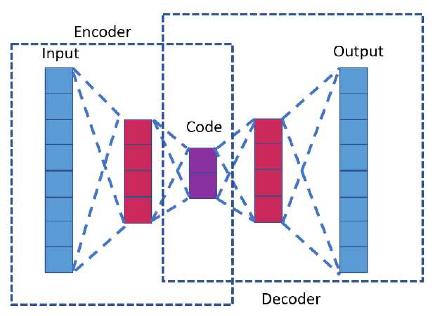
Figure 6.
The encoder–decoder LSTM model.
Figure 6.
The encoder–decoder LSTM model.
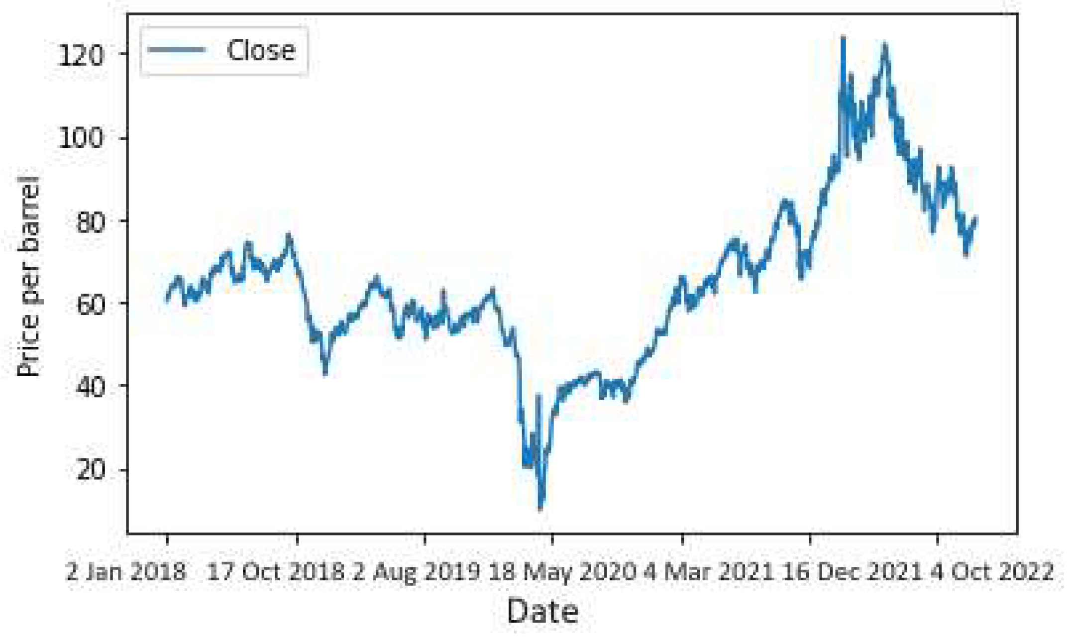
Figure 7.
Daily crude oil prices for the long-term period.
Figure 7.
Daily crude oil prices for the long-term period.
Figure 8.
Daily crude oil prices for the medium-term period.
Figure 8.
Daily crude oil prices for the medium-term period.
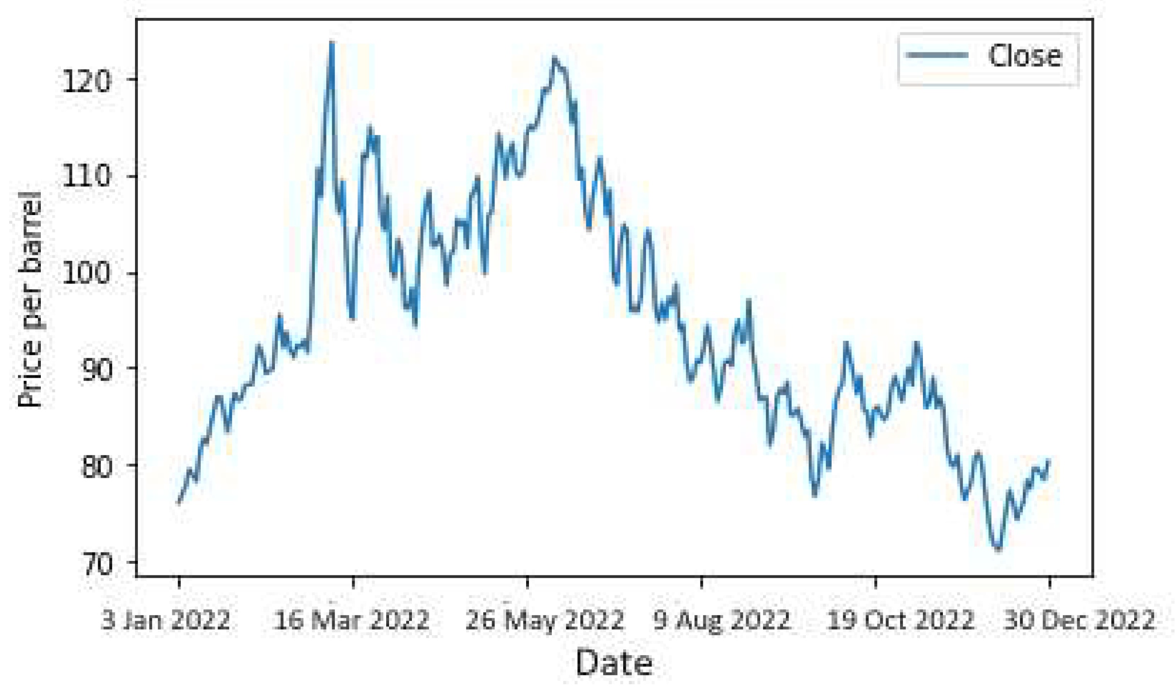
Figure 9.
Daily crude oil prices for the short-term period.
Figure 9.
Daily crude oil prices for the short-term period.
Figure 10.
The training and testing data for long-, medium-, and short-term datasets.
Figure 10.
The training and testing data for long-, medium-, and short-term datasets.
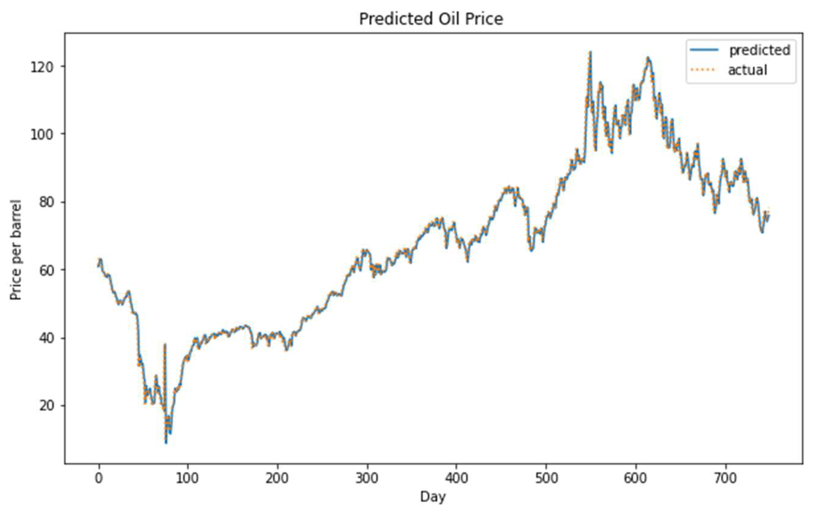
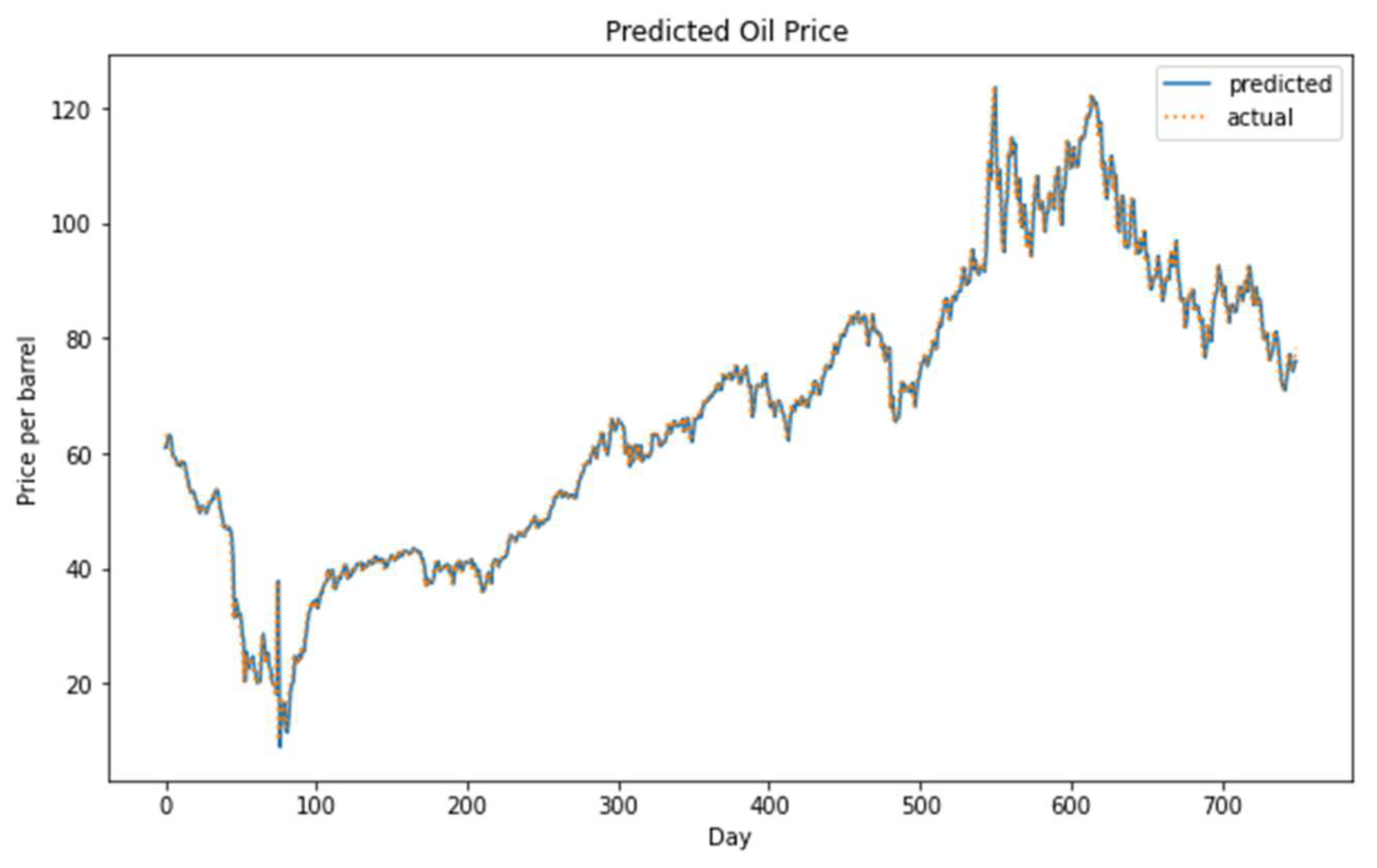
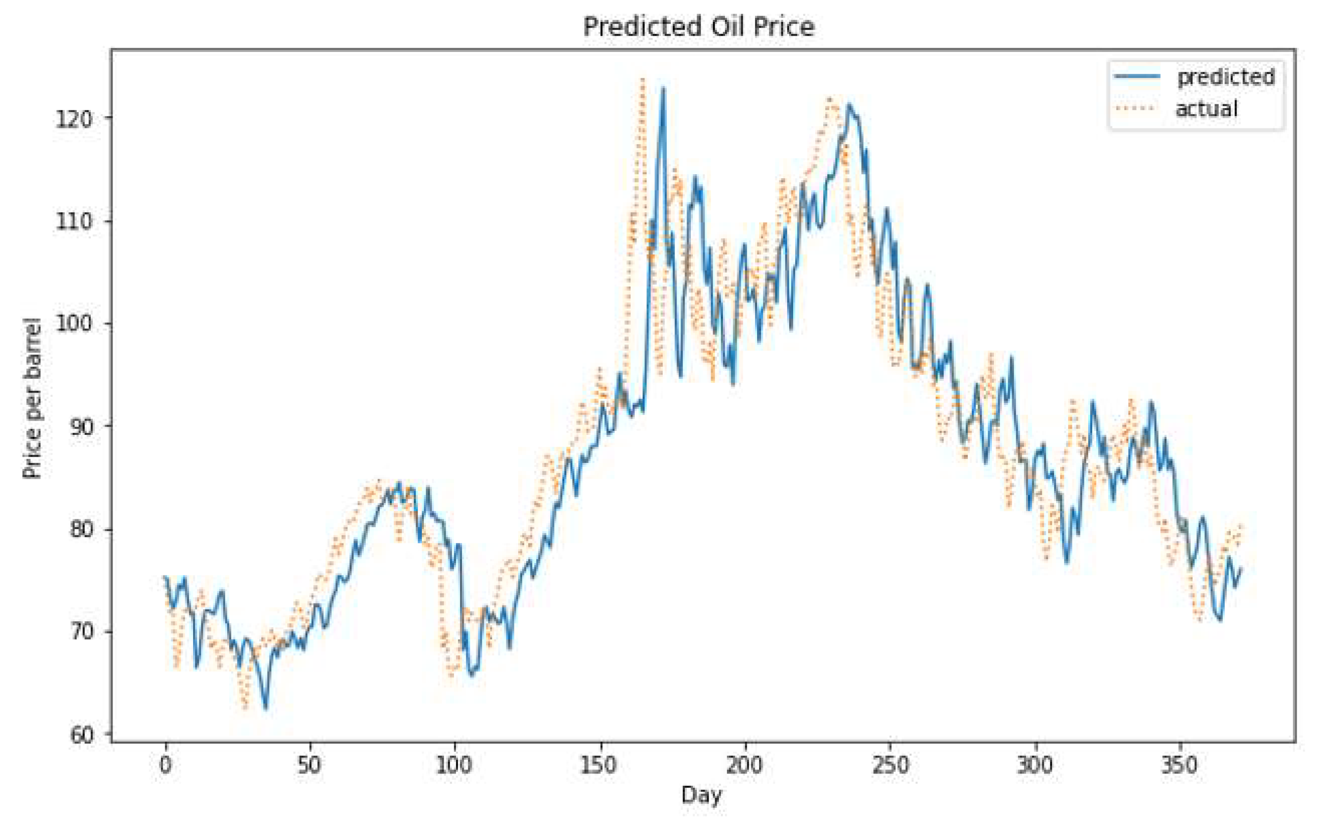
Figure 11.
The actual versus the predicted oil price using the hybrid model on the long-term dataset.
Figure 11.
The actual versus the predicted oil price using the hybrid model on the long-term dataset.
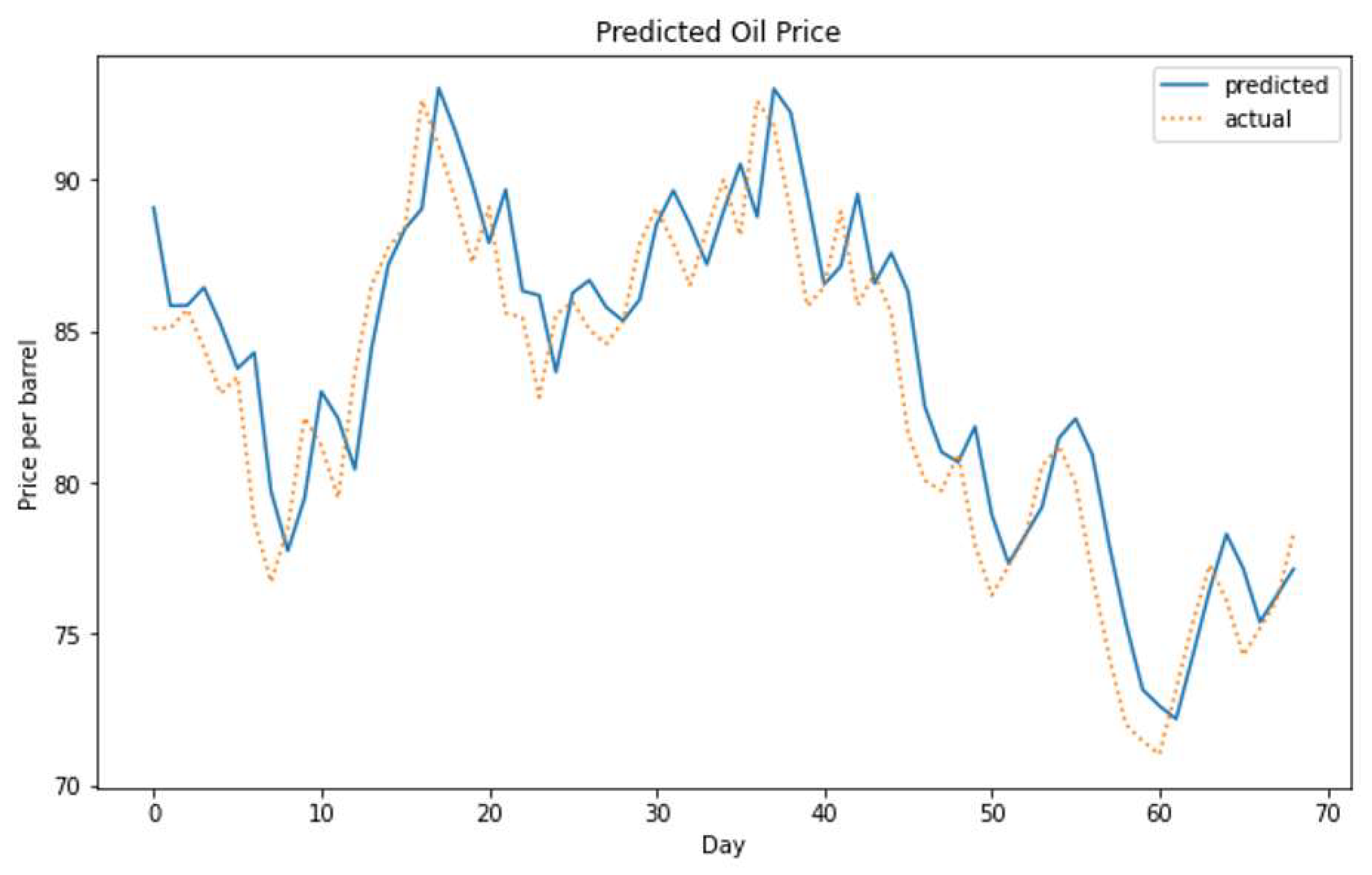
Figure 12.
The actual versus the predicted oil price using the hybrid model on the medium-term dataset.
Figure 12.
The actual versus the predicted oil price using the hybrid model on the medium-term dataset.
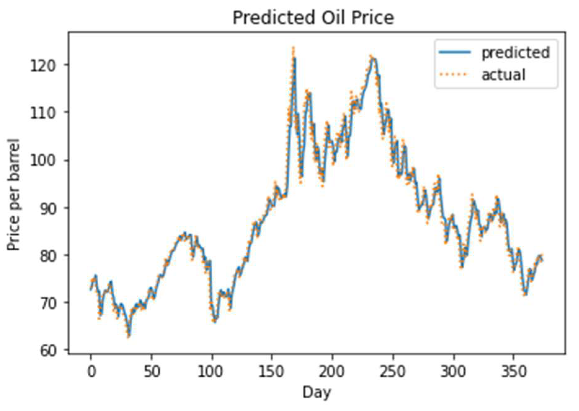
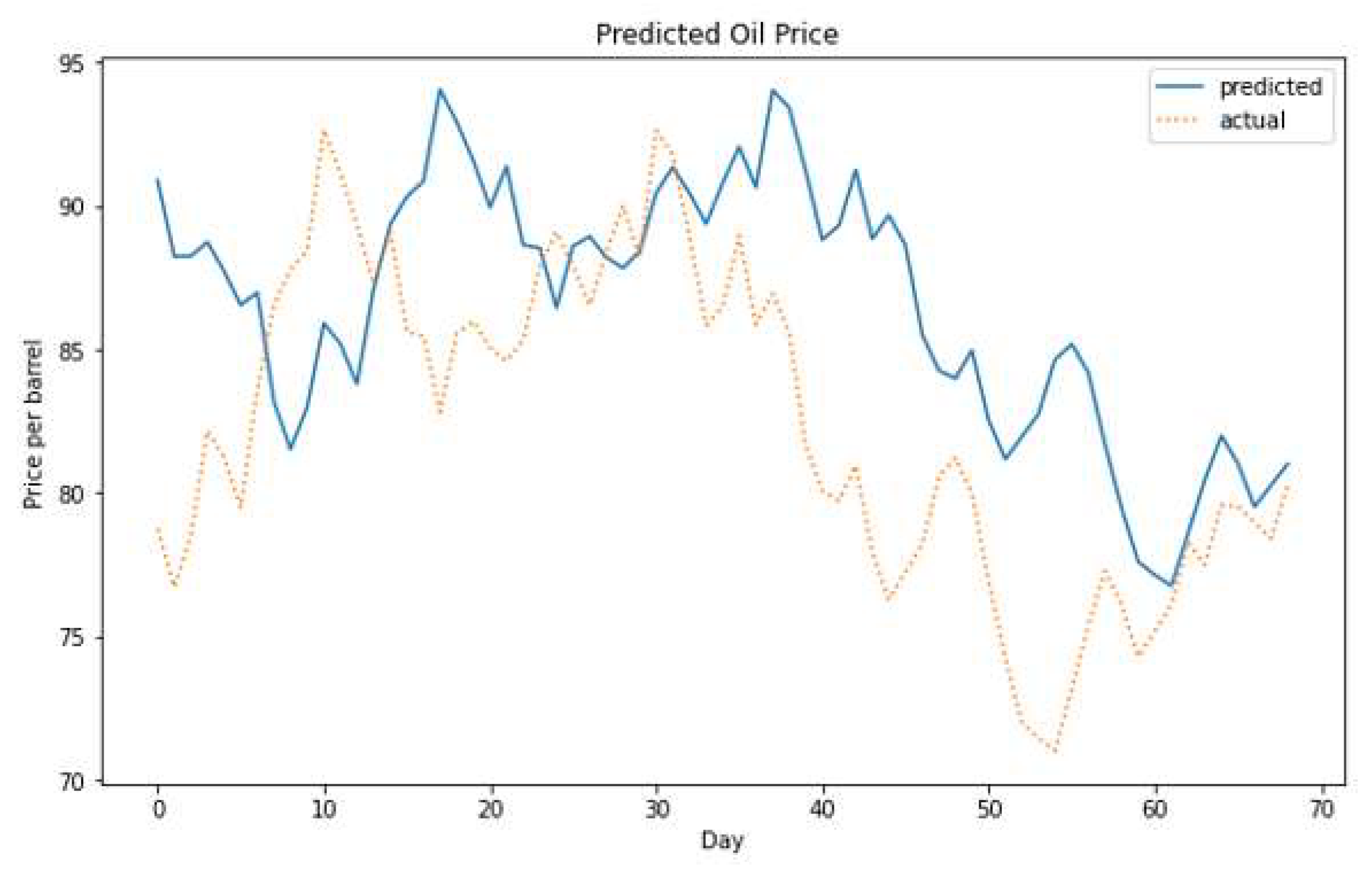
Figure 13.
The actual versus the predicted oil price using the hybrid model on the short-term dataset.
Figure 13.
The actual versus the predicted oil price using the hybrid model on the short-term dataset.
Figure 14.
(a) Simple moving average of the actual prices versus the predicted prices on the short-term dataset. (b) Simple moving average of the actual prices versus the predicted prices on medium-term dataset.
Figure 14.
(a) Simple moving average of the actual prices versus the predicted prices on the short-term dataset. (b) Simple moving average of the actual prices versus the predicted prices on medium-term dataset.
Figure 15.
Simple moving average of the actual prices versus the predicted prices on the long-term dataset with an enlarged view of six time-intervals.
Figure 15.
Simple moving average of the actual prices versus the predicted prices on the long-term dataset with an enlarged view of six time-intervals.
Figure 16.
The actual versus the predicted oil price, using the vector output CNN–LSTM model on the long-term dataset for the t+1 day price prediction.
Figure 16.
The actual versus the predicted oil price, using the vector output CNN–LSTM model on the long-term dataset for the t+1 day price prediction.
Figure 17.
The actual versus the predicted oil price, using the encoder–decoder model on the long-term dataset for the t+1 day price prediction.
Figure 17.
The actual versus the predicted oil price, using the encoder–decoder model on the long-term dataset for the t+1 day price prediction.
Figure 18.
The actual versus the predicted oil price, using the vector output CNN–LSTM model on the long-term dataset for the t+7 day price prediction.
Figure 18.
The actual versus the predicted oil price, using the vector output CNN–LSTM model on the long-term dataset for the t+7 day price prediction.
Figure 19.
The actual versus the predicted oil price, using the encoder–decoder LSTM model on the long-term dataset for the t+7 day price prediction.
Figure 19.
The actual versus the predicted oil price, using the encoder–decoder LSTM model on the long-term dataset for the t+7 day price prediction.
Figure 20.
The actual versus the predicted oil price, using the vector output CNN–LSTM model on the medium-term dataset for the t+1 day price prediction.
Figure 20.
The actual versus the predicted oil price, using the vector output CNN–LSTM model on the medium-term dataset for the t+1 day price prediction.
Figure 21.
The actual versus the predicted oil price, using the encoder–decoder model on the medium-term dataset for the t+1 day price prediction.
Figure 21.
The actual versus the predicted oil price, using the encoder–decoder model on the medium-term dataset for the t+1 day price prediction.
Figure 22.
The actual versus the predicted oil price, using the vector output CNN–LSTM model on the medium-term dataset for the t+7 day price prediction.
Figure 22.
The actual versus the predicted oil price, using the vector output CNN–LSTM model on the medium-term dataset for the t+7 day price prediction.
Figure 23.
The actual versus the predicted oil price, using the encoder–decoder LSTM model on the medium-term dataset for the t+7 day price prediction.
Figure 23.
The actual versus the predicted oil price, using the encoder–decoder LSTM model on the medium-term dataset for the t+7 day price prediction.
Figure 24.
The actual versus the predicted oil price, using the vector output CNN–LSTM model on the short-term dataset for the t+1 day price prediction.
Figure 24.
The actual versus the predicted oil price, using the vector output CNN–LSTM model on the short-term dataset for the t+1 day price prediction.
Figure 25.
The actual versus the predicted oil price, using the encoder–decoder model on the short-term dataset for the t+1 day price prediction.
Figure 25.
The actual versus the predicted oil price, using the encoder–decoder model on the short-term dataset for the t+1 day price prediction.
Figure 26.
The actual versus the predicted oil price, using the vector output CNN–LSTM model on the short-term dataset for the t+7 day price prediction.
Figure 26.
The actual versus the predicted oil price, using the vector output CNN–LSTM model on the short-term dataset for the t+7 day price prediction.
Figure 27.
The actual versus the predicted oil price, using the encoder–decoder LSTM model on the short-term dataset for the t+7 day price prediction.
Figure 27.
The actual versus the predicted oil price, using the encoder–decoder LSTM model on the short-term dataset for the t+7 day price prediction.
Table 1.
Statistical properties of crude oil prices (2013–2022).
Table 1.
Statistical properties of crude oil prices (2013–2022).
| Mean | Std. Dev. | Skewness | Kurtosis |
|---|
| 65.78 | 22.49 | 0.44 | 0.82 |
Table 2.
Statistical properties of crude oil prices (2018–2022).
Table 2.
Statistical properties of crude oil prices (2018–2022).
| Mean | Std. Dev. | Skewness | Kurtosis |
|---|
| 64.75 | 19.77 | 0.39 | 0.40 |
Table 3.
Statistical properties of crude oil prices (2022).
Table 3.
Statistical properties of crude oil prices (2022).
| Mean | Std. Dev. | Skewness | Kurtosis |
|---|
| 94.3 | 12.36 | 0.36 | −0.77 |
Table 4.
RMSE of various optimizers versus activation functions. The lowest RMSE is highlighted in the bold font.
Table 4.
RMSE of various optimizers versus activation functions. The lowest RMSE is highlighted in the bold font.
| | Adam | Nadam | Adadelta | Adagrad | Adamax | Ftrl | RMSprop |
|---|
| ELU | 2.45 | 2.42 | 3.82 | 3.36 | 2.39 | 3.5 | 3.06 |
| ReLU | 2.47 | 2.36 | 3.48 | 3.35 | 2.5 | 3.5 | 3.16 |
| SELU | 2.6 | 2.4 | 3.54 | 2.76 | 2.45 | 3.27 | 3.05 |
| tanh | 3.10 | 2.95 | 36.62 | 56.77 | 2.97 | 53.91 | 3.06 |
| Softplus | 2.51 | 2.44 | 3.68 | 3.10 | 2.42 | 3.37 | 2.55 |
| Softsign | 3.11 | 3.36 | 40.32 | 59.91 | 3.32 | 61.70 | 4.05 |
Table 5.
RMSE and MAPE of each model on the long-term dataset. The lowest RMSE and MAPE are highlighted in the bold font.
Table 5.
RMSE and MAPE of each model on the long-term dataset. The lowest RMSE and MAPE are highlighted in the bold font.
| Dataset (2013–2022) | RMSE | MAPE |
|---|
| Vanilla LSTM | 2.51 | 3.0% |
| Stacked LSTM | 2.52 | 3.0% |
| CNN–LSTM | 2.36 | 2.7% |
| SVM | 2.87 | 3.9% |
| CNN | 2.54 | 2.9% |
| ARIMA | 2.50 | 2.8% |
Table 6.
RMSE and MAPE of each model on the medium-term dataset. The lowest RMSE and MAPE are highlighted in the bold font.
Table 6.
RMSE and MAPE of each model on the medium-term dataset. The lowest RMSE and MAPE are highlighted in the bold font.
| Dataset (2018–2022) | RMSE | MAPE |
|---|
| Vanilla LSTM | 2.88 | 2.3% |
| Stacked LSTM | 2.88 | 2.2% |
| CNN–LSTM | 2.75 | 2.1% |
| SVM | 19.7 | 12.9% |
| CNN | 2.82 | 2.3% |
| ARIMA | 3.06 | 2.5% |
Table 7.
RMSE and MAPE of each model on the short-term dataset. The lowest RMSE and MAPE are highlighted in the bold font.
Table 7.
RMSE and MAPE of each model on the short-term dataset. The lowest RMSE and MAPE are highlighted in the bold font.
| Dataset (2022) | RMSE | MAPE |
|---|
| Vanilla LSTM | 2.72 | 2.7% |
| Stacked LSTM | 2.81 | 2.8% |
| CNN–LSTM | 2.18 | 2.2% |
| SVM | 2.58 | 2.6% |
| CNN | 2.35 | 2.4% |
| ARIMA | 2.35 | 2.3% |
Table 8.
RMSE of each model on the long-term dataset over seven consecutive days. The lowest RMSE is highlighted in the bold font.
Table 8.
RMSE of each model on the long-term dataset over seven consecutive days. The lowest RMSE is highlighted in the bold font.
| Day | 1 | 2 | 3 | 4 | 5 | 6 | 7 |
|---|
| CNN | 3.65 | 4.22 | 4.66 | 5.04 | 5.32 | 5.63 | 5.83 |
| LSTM | 2.79 | 3.59 | 4.19 | 4.52 | 4.93 | 5.24 | 5.49 |
| CNN–LSTM | 2.54 | 3.29 | 3.89 | 4.39 | 4.87 | 5.21 | 5.48 |
| Encoder–Decoder | 2.48 | 3.54 | 5.01 | 7.00 | 9.86 | 13.90 | 21.08 |
Table 9.
RMSE of each model on the medium-term dataset over seven consecutive days. The lowest RMSE is highlighted in the bold font.
Table 9.
RMSE of each model on the medium-term dataset over seven consecutive days. The lowest RMSE is highlighted in the bold font.
| Day | 1 | 2 | 3 | 4 | 5 | 6 | 7 |
|---|
| CNN | 4.02 | 4.71 | 5.27 | 5.81 | 6.16 | 6.37 | 6.58 |
| LSTM | 3.15 | 3.96 | 4.83 | 5.48 | 6.08 | 6.37 | 6.86 |
| CNN–LSTM | 2.74 | 3.83 | 4.58 | 5.19 | 5.78 | 6.21 | 6.46 |
| Encoder–Decoder | 2.74 | 4.00 | 4.72 | 5.43 | 5.97 | 6.36 | 6.61 |
Table 10.
RMSE of each model on the short-term dataset over seven consecutive days. The lowest RMSE is highlighted in the bold font.
Table 10.
RMSE of each model on the short-term dataset over seven consecutive days. The lowest RMSE is highlighted in the bold font.
| Day | 1 | 2 | 3 | 4 | 5 | 6 | 7 |
|---|
| CNN | 3.59 | 4.13 | 4.65 | 5.04 | 5.29 | 5.46 | 5.73 |
| LSTM | 4.36 | 5.21 | 6.52 | 6.30 | 6.81 | 7.43 | 7.35 |
| CNN–LSTM | 2.60 | 3.43 | 4.10 | 4.64 | 4.96 | 5.28 | 5.49 |
| Encoder–Decoder | 2.42 | 4.04 | 5.14 | 6.17 | 7.11 | 8.00 | 8.60 |
Table 11.
MAPE of each model on the long-term dataset over seven consecutive days. The lowest MAPE is highlighted in the bold font.
Table 11.
MAPE of each model on the long-term dataset over seven consecutive days. The lowest MAPE is highlighted in the bold font.
| Day | 1 | 2 | 3 | 4 | 5 | 6 | 7 |
|---|
| CNN | 4.25% | 4.94% | 5.45% | 5.96% | 6.53% | 6.98% | 7.34% |
| LSTM | 3.25% | 4.17% | 4.84% | 5.23% | 5.73% | 6.15% | 6.47% |
| CNN–LSTM | 2.75% | 3.66% | 4.52% | 5.09% | 5.60% | 6.01% | 6.49% |
| Encoder–Decoder | 2.66% | 4.08% | 5.11% | 5.79% | 6.37% | 6.87% | 7.34% |
Table 12.
MAPE of each model on the medium-term dataset over seven consecutive days. The lowest MAPE is highlighted in the bold font.
Table 12.
MAPE of each model on the medium-term dataset over seven consecutive days. The lowest MAPE is highlighted in the bold font.
| Day | 1 | 2 | 3 | 4 | 5 | 6 | 7 |
|---|
| CNN | 3.38% | 3.98% | 4.38% | 4.74% | 5.08% | 5.43% | 5.75% |
| LSTM | 2.56% | 3.36% | 4.10% | 4.62% | 5.11% | 5.33% | 5.96% |
| CNN–LSTM | 2.20% | 3.16% | 3.79% | 4.29% | 4.63% | 5.06% | 5.47% |
| Encoder–Decoder | 2.28% | 3.49% | 4.11% | 4.73% | 5.10% | 5.48% | 5.81% |
Table 13.
MAPE of each model on the short-term dataset over seven consecutive days. The lowest MAPE is highlighted in the bold font.
Table 13.
MAPE of each model on the short-term dataset over seven consecutive days. The lowest MAPE is highlighted in the bold font.
| Day | 1 | 2 | 3 | 4 | 5 | 6 | 7 |
|---|
| CNN | 3.61% | 4.15% | 4.67% | 5.24% | 5.44% | 5.61% | 5.88% |
| LSTM | 4.13% | 4.96% | 6.29% | 5.98% | 6.56% | 7.10% | 6.96% |
| CNN–LSTM | 2.55% | 3.38% | 3.88% | 4.31% | 4.63% | 5.07% | 5.39% |
| Encoder–Decoder | 2.34% | 3.87% | 4.76% | 5.77% | 6.72% | 7.63% | 8.27% |


_Zheng.png)


