Abstract
The Thailand Futures Exchange launched USD Futures as the first currency futures contract on 5 June 2012. However, it has been available for night trading since 27 September 2021. This research aims to analyze the effect of adding a night trading session on USD Futures market liquidity and to make a liquidity comparison between day and night session trading. By adding a dummy variable into the vector autoregression model of order 5 to capture the effect of a night session introduction on market liquidity, the results show that market depth and breadth are even stronger after a longer trading session. In addition, the t-test results show the presence of lower tightness but stronger depth and breadth in day session trading than in night session trading, because of the availability of a large number of orders and the ability of the market to have smoother trading in day as opposed to night. Due to the positive effect of extended trading hours on market depth and breadth, TFEX should consider a longer night session in line with other global futures markets. Night traders should also be aware of liquidity risk due to low night session trading volume.
1. Introduction
Over the past two decades, the Thailand Futures Exchange (TFEX) continued to develop new products and services to keep pace with investor demands, as well as boosting trading liquidity. To help traders hedge and speculate on the fluctuation of exchange rates, the TFEX launched USD Futures as the first currency derivatives product on 5 June 2012. The regular trading hours of USD Futures starts from 9:45 a.m.–4:55 p.m., which differs from the trading hours for foreign assets in different time zones. Major international futures markets already offer almost 24 h trading. The Singapore Exchange is an example of a market that extends hours for trading certain derivatives. The extension allows traders to execute derivatives on the Singapore Exchange until 05:15 Singapore time of the following day. The Taiwan Futures Exchange also launches after-hours trading session to allow traders to trade until 5:00 the next morning. The after-hours platform enhances futures market’s international competitiveness and provides investors with a comprehensive hedging channel and more trading opportunities. As evidenced by Jiang et al. (2020), trading activity, as measured by volume, turnover, and open interest, is higher after the introduction of a night trading session by the Shanghai Futures Exchange for gold and silver futures.
The TFEX started to launch night session of gold and silver futures on 20 June 2011. Following precious metals derivatives, the TFEX extended the trading hours of USD Futures on 27 September 2021 to align with the practices of major international markets. The launch of the night trading session during 6:50 p.m.–11:55 p.m. allows traders to speculate and hedge against foreign exchange movement more conveniently and efficiently. The higher volatility in exchange rate and the extended trading hours of USD Futures led to an increase in its trading volume in the last three years. As shown in Table 1, the trading volume of USD Futures moved down and up for almost a decade. However, it showed the biggest jump (316.48 percent) in 2020 to 2,803,128 contracts with an open interest of 44,059 contracts at the end of the year due to the COVID-19 pandemic impacting global markets and volatility. Since then, it has grown continuously to surpass the 10 million mark in 2022: a 191.57 percent surge in yearly trading volume. Overall, the open interest at the end of December 2022 soared 55.20 percent from a year earlier to 179,188 contracts. For the first time in over a decade, the TFEX has made it to the top ten currency derivative exchanges based on trading volume in 2022.

Table 1.
Yearly trading volume and open interest of USD Futures.
The launch of the night trading session is one of the most important developments in the USD Futures market. With a longer trading session, USD Futures has become an alternative hedging tool for traders who invest in foreign assets and want to manage exchange rate risk outside of commercial banks’ business hours. However, there are a number of factors that investors should be aware of when trading outside of regular hours. For example, there may be fewer traders involved with nighttime trading, leading to a lot less liquidity than during day trading session. As such, the primary focus of this study is to examine the effect of adding night trading session on the USD Futures’ market liquidity and to make a liquidity comparison between day and night session trading. The current study adds to the existing literature on liquidity measurement based on daily data in futures market. In addition, most studies in regular and after-hours trading focus on equity and commodity futures markets. To the best of our knowledge, the effect of adding a night trading session on liquidity has never been examined in the context of currency derivatives before. A better understanding of the USD Futures’ market liquidity, given an extension of trading hours, is crucial, since it will help the TFEX and other derivative exchanges in developing and promoting new products and services. It also helps investors make informed decisions and manage the risks associated with their investment.
The remainder of this paper is conducted as follows. Section 2 provides an overview of existing literature on the measurement of liquidity and the effect of night trading. Data and methodology are presented in Section 3. Section 4 discusses the estimation results and Section 5 summarizes the main findings and concludes this paper.
2. Literature Review
In this section, we begin by presenting various measures of liquidity. We next conduct a review of the empirical literature on liquidity, with emphasis on stock markets, fixed income markets, and futures markets. We finally investigate the link between night trading and liquidity, with an emphasis on futures markets.
Previous literature on the measurement of market liquidity across five dimensions, namely tightness, immediacy, depth, breadth, and resiliency, can be found in Sarr and Lybek (2002), Broto and Lamas (2020), and Díaz and Escribano (2020).
Tightness is linked to the expenses associated with the execution of a trade. Le and Gregoriou (2020) explained a decomposition of trading costs into two categories, namely explicit and implicit costs. Explicit costs include order processing costs, taxes, and brokerage fees, while implicit costs are bid–ask spreads, size of transaction, and timing of trade execution. Higher transaction costs are related to lower liquidity when market participants reduce their demand for trading and concentrate on a few transactions to avoid larger costs. Some proxies for tightness include Effective Bid-Ask Spread (EBS) and Percentage Spread (PS). According to Roll (1984), given market efficiency, EBS as an estimate of the PS is given by where is the first-order serial covariance of returns. PS is calculated by the spread over the average between bid price (Pb) and ask prices (Pa), .
Immediacy refers to the ability or the speed with which transactions can be executed and settled. It reflects the system efficiency in terms of trading, clearing, and settlement. Wanzala (2018) use the Coefficient of Elasticity of Trading (CET) to assess market immediacy. As introduced by Datar (2000), CET is computed as a ratio of the absolute value of percentage change in trading volume to the absolute value of percentage change in price, . A higher value of CET represents a higher level of immediacy.
Depth is related to the number of orders. Trading volume is the most used trading frequency proxy to assess liquidity. A higher trading volume indicates a deep market and reveals higher liquidity, since it shows how easier it is to execute large orders without moving the market.
Breadth represents the market ability to smoothly enable trading of a given volume of securities with a minimal influence on prices. The Amihud Illiquidity Ratio (IR) proposed by Amihud (2002) is one of the most widely used proxies for market breadth. It is given by a ratio of the absolute return to the dollar volume traded, . A lower IR means a wide market breadth and represents high liquidity.
Resiliency is a market characteristic, such that new orders flow quickly to correct market imbalances. To capture market resiliency, Hasbrouck and Schwartz (1988) proposed the Market Efficiency Coefficient (MEC) as a ratio between the variances of two returns with different time spans, where R is weekly returns and r is daily returns. When this ratio is closer to one, it conveys higher liquidity and a more efficient market.
Table 2 summarizes the liquidity measures to be used for the purpose of this analysis. When examining the effect of adding a night trading session on USD Futures market liquidity, this paper measures market tightness for the whole trading day by using Percentage Spread, which expresses daily spread as a percentage of the midpoint of the bid and ask prices. For a liquidity comparison between day and night session trading, Effective Bid-Ask Spread, as proposed by Roll (1984), is employed for measuring market tightness during day and night sessions due to the limit in obtaining day and night session data to calculate Percentage Spread. The last price data for day and night sessions are obtained to estimate the autocovariance measure of Roll (1984).
Table 2.
Measurement of market liquidity.
In addition, liquidity measures can be classified by data frequency. According to Le and Gregoriou (2020), liquidity proxies are separated into two groups, namely high-frequency (intraday) and low-frequency (daily) measures. The use of low frequency measures in research and practice has become more widely accepted because of the availability of data and simplicity.
Empirical studies employ numerous measures to analyze liquidity in a wide set of products and geographical regions. Several studies use low-frequency measures and focus on stock market liquidity. For example, Amihud (2002) analyzed the effect of illiquidity, defined as the average ratio of the daily absolute return to the dollar trading volume, on stock returns using data from New York Stock Exchange in the years 1963–1997. The results show that expected market illiquidity has a positive and significant effect on ex ante stock excess return, and unexpected illiquidity has a negative and significant effect on contemporaneous stock return. Both expected and unexpected illiquidity effects are shown to be stronger for small firms’ stocks. Wanzala (2018) proposed a new measure of market immediacy and conducted OLS regression analysis using data from 2001 to 2016 from the Nairobi Securities Exchange and Kenya National Bureau of Statistics. The findings show a negative impact of inflation and a positive impact of market immediacy on economic growth. Naik et al. (2020) employed Vector Auto Regressive (VAR) of the order 2 model to analyze the simultaneous relationships among four liquidity dimensions, namely depth, breadth, tightness, and immediacy, using data of 500 stocks in an Indian stock market from 2009 to 2019. There exists a negative relation between depth and tightness at the significance level of 0.01. Immediacy is found to be independently determined in the market. Xie et al. (2022) analyzed the determinants of stock liquidity in the Chinese market from January 2003 to September 2021. They used trading volume, Amihud’s illiquidity ratio, Roll’s price impact, and the quoted relative bid–ask spread as proxies for stock liquidity. Their findings show a positive relation between systematic return and stock liquidity and a negative relation between idiosyncratic variance and stock liquidity.
The vast literature is focused on the treasury and corporate bond markets. For example, Trebbi and Xiao (2019) employed a large set of liquidity proxies, including the Amihud measure, imputed round-trip cost, Roll measure, non-block trades, size, turnover, zero trading days, variability of Amihud, and variability of imputed round-trip cost, with emphasis on the U.S. corporate bond market. They found no systematic evidence of deterioration in liquidity levels or structural breaks during the period of regulatory intervention. Broto and Lamas (2020) focused on liquidity resilience of the US treasury debt by proposing liquidity volatility, rather than liquidity level, as the key variable to characterize resilience. They employed a bivariate CC-GARCH model to relate the volatility of five liquidity measures to returns volatility of the 10-year US Treasury note, using data from January 2003 to June 2016. The findings show that after the great financial crisis of 2007–2009, volatility persistence is lower, which is consistent with a lower resilience.
The empirical papers mentioned so far examine liquidity in stock markets and fixed income markets. In the case of future markets, Woo and Kim (2021) used low-frequency measures and employ regression models to investigate the effect of the National Pension Service (NPS)’s trading KOSPI200 futures on the returns, the liquidity and the volatility in both the futures market and the stock market. They use the recent ten years’ transaction data during the period from January 2010 to March 2020 and measure liquidity using trading amount and the Amihud measure. Their findings show that the NPS’s net investment flow in the KOSPI200 futures market improves the liquidity of the KOSPI market and reduces the volatility of both the KOSPI200 futures market and the KOSPI market. The NPS’s net investment flow in the KOSPI200 futures market shows the return predictability about both KOSPI200 futures and KOSPI200 spot index. Using the data of gold coin futures contracts in the Iran Mercantile Exchange from 2017 to August 2018, Basirian and Sehatpour (2021) analyzed how the volume of transactions, price volatility, and futures price affect liquidity, measured by bid-ask spread and market depth. The empirical results provides evidence of a positive impact of price volatility on market dept at the significance level of 0.01. Other factors do not show any significant impact on liquidity. In addition, another group of existing literature uses high-frequency measures to evaluate liquidity in the futures market. For example, Fett and Haynes (2017) calculated multiple liquidity measures, including bid-ask spreads, orderbook depth, and other metrics related to trading costs and execution quality for three active futures products (S&P E-mini, ten year treasuries and WTI crude oil) from 2013 through mid-2016. Trends for a few of these liquidity measures signal a potential increase in trading costs over the last few years such as reduced trade sizes and, in cases, reductions in orderbook depth, especially for the E-mini contract. Reductions in orderbook depth often coincide with periods of enlarged market volatility. Like orderbook depth, bid-ask spreads for WTI crude oil have increased during the volatile late-2014 period. In contrast, WTI crude oil trading volumes have increased since around mid-2015.
While several studies measure and analyze liquidity for individual assets, another group of research focuses on liquidity commonality, which is liquidity co-movements across assets or markets. Over the sample period from January 2000 to April 2010, Wang (2010) showed that liquidity commonality across 12 Asian stock markets is much higher when measured relative to a set of regional and global factors instead of the single factor. Regional factors affect liquidity commonality through shocks in liquidity and volatility, while global factors affect liquidity commonality through return and volatility. Cross-market liquidity commonality in Asia increased significantly during and after the recent global financial crisis. In the fixed income market, Panagiotou et al. (2022) empirically examined the determinants of liquidity commonality in the European sovereign bond over a period of 2011–2018. They calculated four liquidity measures, namely quoted spreads and depths, effective spreads and the Amihud ratio, and used the adjusted R2 of regressions of the liquidity of individual bonds on market-wide liquidity as a measure of liquidity commonality. There is strong evidence of liquidity commonality at the national level in all four liquidity measures, with quoted spreads and depths exhibiting strong co-movements.
There are some studies investigating market liquidity in the presence of nighttime trading. For example, Jiang et al. (2020) used three liquidity measures, including Roll measure, Amihud illiquidity measure, and the proportion of zero returns, to examine the liquidity of gold and silver futures at the Shanghai Futures Exchange (SHFE) before and after the introduction of night trading. Their findings show that the introduction of night trading significantly improves the volume and liquidity of gold and silver futures in China. In particular, the improvement in liquidity, as captured by Roll measure and Amihud illiquidity measure, suggests a decrease in transaction costs and a lesser price impact. Other studies also focus on the effect of introducing a night trading session at the Chinese futures market (see, e.g., Fung et al. 2016; Klein and Todorova 2021; Yao et al. 2021). However, to the best of our knowledge, the liquidity changes brought by the introduction of nighttime trading to currency futures market have not been addressed in previous literature. Therefore, this paper adds to the existing literature on the effects of night trade on currency futures market liquidity, especially in a Thai context.
3. Data and Methodology
This paper uses the daily data of USD Futures, such as settlement price, last price, bid price, ask price, and trading volume, from SETSMART for a period starting from 2 January 2020 to 30 December 2022, covering the period before and after the extended trading hour (night session) of USD Futures on 27 September 2021. The Thailand Futures Exchange (TFEX) sets the settlement months (expiry months) of USD Futures to the three nearest consecutive months plus the next quarterly months. However, the most active contract month is the quarterly month. As shown in Figure 1 and Figure 2, the quarterly month contracts have the highest average daily trading volume and average daily number of transactions. In addition, since the introduction of night session trading, the average trading volume of the quarterly month contracts has exceeded 10,000 contracts per day, and its average number of transactions has been above 600 deals per day. Therefore, this paper uses daily price data from the quarterly month contracts to construct the USD Futures price data set. Following Ripple and Moosa (2009), both the daily trading volume and open interest are used as a two-criterion test to determine when to switch from the contract, which is close to expiration, to another contract in a further-out month. The USD Futures price data set is then created by switching or rolling over from the expiring quarterly month contract to the next quarterly month contract when trading volume and open interest of the expiring quarterly month contract are lower than those of the next quarterly month contract. For example, the constructed series of USD Futures price start with the March 2020 USD Futures on 2 January 2020, then switch to the next quarterly month contract, the June 2020 USD Futures, when the trading volume and open interest of the March 2020 USD Futures are lower than those of the June 2020 USD Futures. It is rolled over to the September 2020 USD Futures when the trading volume and open interest of the June 2020 USD Futures are lower than those of the September 2020 USD Futures. The process continues until the prices of USD Futures on 30 December 2022 are collected from the March 2023 USD Futures.
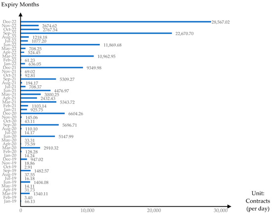
Figure 1.
Average daily trading volume of USD Futures by expiry months.
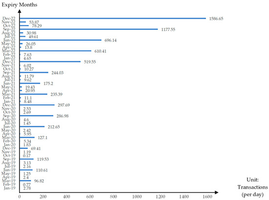
Figure 2.
Average daily number of transactions of USD Futures by expiry months.
Based on the data, this paper computes market liquidity measures across five dimensions, namely tightness, immediacy, depth, breadth, and resiliency, as shown in Table 2. As suggested by Naik et al. (2020), this paper uses Percentage Spread as a measure of market tightness, Coefficient of Elasticity of Trading as a measure of market immediacy, and Amihud Illiquidity Ratio as a measure of market breadth. The Effective Bid-Ask Spread is also employed as a proxy of market tightness (see Broto and Lamas 2020; Jiang et al. 2020). Following Broto and Lamas (2016), the trading volume and market efficiency coefficient are used to analyze market depth and resiliency, respectively. The USD Futures return (r) is obtained by taking the difference of natural log of USD Futures prices (P), rt = ln Pt − ln Pt−1. For a liquidity comparison between day and night session trading, the USD Futures returns (r) and the absolute value of percentage change in USD Futures price (%∆P) during day session and night session are computed using the last prices during day session and night session, respectively. On the other hand, the settlement price is used to represent the entire daily trading session when examining the effect of adding night trading session on USD Futures market liquidity.
Following Naik et al. (2020), this study assumes the existence of positive interdependency between Market Tightness (MT), Market Immediacy (MI), Market Depth (MD), Market Breadth (MB), and Market Resiliency (MR). Therefore, the Vector Autoregressive (VAR) model is employed for the simultaneous relationships among five liquidity dimensions. Then, the dummy variable (NT) is added into the VAR model to capture the effect of night session introduction on market liquidity. This paper picks the optimal lag order 5 in the VAR due to the minimum Hannan–Quinn Criterion (HQ) and Schwarz Criterion (SC). The VAR(5) model can be written as follows:
To make a comparison of USD Futures market liquidity between day session trading and night session trading, the dependent samples t-test is used for testing the mean difference in all five liquidity dimensions of day session trading and night session trading.
where D is difference in USD Futures market liquidity between day session trading and night session trading and n is the size of the sample. The degrees of freedom can be calculated as n − 1.
The null hypothesis (H0) is that the mean difference in USD Futures market liquidity during day session and night session is zero. In another word, there is no difference in USD Futures market liquidity during the day session and night session.
The alternative hypothesis (Ha) is that the mean difference in the USD Futures’ market liquidity during the day session and night session is different from zero. In another word, there is a difference in USD Futures’ market liquidity during day session and night session.
4. Results and Discussion
Table 3 presents the Augmented Dickey–Fuller (ADF) test results and the mean value of the liquidity measures from 2 January 2020 to 30 December 2022. The ADF test is conducted to evaluate whether the time series are stationary or not. Table 3 shows that all five liquidity measures are stationary at the 5 percent level of significance. Market Tightness (MT), measured by percentage spread, has the average value of 0.0446 percent. A narrow percentage spread would indicate lower transaction costs and higher liquidity through a tighter market. To measure Market Immediacy (MI), this study uses the coefficient of elasticity of trading, which has the average value of 375.4520. A larger value of the coefficient of elasticity of trading implies a higher immediacy and thus confirms higher market liquidity. Market Depth (MD) is measured by trading volume (unit: 10,000 contracts), which is the most used trading frequency proxy to assess liquidity. The average trading volume of USD Futures is 23,090 contracts per day. A higher trading volume implies a deep market and shows higher liquidity. For measuring Market Breadth (MB), this paper uses the Amihud illiquidity ratio. Its average value is 0.6277 meaning that a trade of 1 billion baht in USD Futures moves futures price by roughly 0.6277 percent. A lower ratio represents the wide market breadth and thus suggests the existence of high liquidity. To capture Market Resiliency (MR), market efficiency coefficient is used with the average value of 0.9775. When this ratio is closer to one, it conveys a more efficient liquidity resiliency.
Table 3.
ADF unit root results and mean value of the liquidity measures.
To determine if the VAR(5) model gives an adequate description of the data, the Lagrange Multiplier (LM) test is conducted for checking autocorrelation. The LM test statistics is 30.5716 (p-value = 0.2036), so the null hypothesis that there is no autocorrelation left in the residuals for any of the six orders tested cannot be rejected at a confidence interval of 99%. The stability test of the VAR(5) model is also conducted. Figure 3 shows that all the inverse roots of the model have roots with modulus less than one and lie inside the unit circle. The VAR(5) model is variance and covariance stationary, and therefore satisfies the stability condition. It is appropriate for this research. Table 4 presents the estimated results of the VAR(5) model.
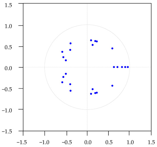
Figure 3.
Inverse roots of AR characteristic polynomial.
Table 4.
Estimation results of the VAR(5) model.
Table 4 shows that the total variations in MT, MI, MD, MB, and MR are explained by the other variables to the extent of 13.02%, 11.63%, 70.73%, 27.70%, and 86.97%, respectively. It is evident that current values of all liquidity measures are positively dependent on one or two days of own lagged values. MT is positively affected by its lagged values and also by one day lag of MB. This suggests that trading costs and the impact on futures price of the earlier periods define the crucial movements in current day costs. MI is found to be dependent on its lagged value and other liquidity dimensions, except MT. This exhibits that the speed of execution is caused by not only its own previous day lag but also the past trading volume, the past price impact, and the past market ability to recover from unexpected shocks. Regarding MD, the estimated results show that the current trading volume is positively affected by its own previous day lags and one day lagged value of MI. This suggests that investors base their trading behavior by referring to the past trading activity. Additionally, past increased immediacy in trade generates more trading volume. The results also show that one day and two day lags of MT are found to positively affect the present values of MB. As suggested by Naik et al. (2020), the increased execution costs will discourage further trades, which, in turn, will result in a higher impact on their prices. Variations in MR are caused by their own past movements and past changed immediacy. By adding the dummy variable (NT) into the VAR(5) model to capture the effect of night session introduction on market liquidity, the results show that the coefficient of NT in the regression equation of MD is positive and statistically significant at 0.05 level. This implies that the current trading volume is positively affected by the night session introduction. The coefficient of NT in the regression equation of MB is also statistically significant at 0.05 level. It is negative since this paper uses the Amihud illiquidity ratio as a measure of MB. After the introduction of the night session, a lower Amihud illiquidity ratio represents the wide market breadth. Therefore, market depth and breadth are even stronger after a longer trading session. It would make sense for the TFEX to respond to increased market liquidity by extending a night session in line with other global futures markets.
Next, this study conducts the VAR Granger causality test to assess the casual relationship between five liquidity dimensions, namely Market Tightness (MT), Market Immediacy (MI), Market Depth (MD), Market Breadth (MB), and Market Resiliency (MR). As shown in Table 5, Granger causality results support the patterns observed in the VAR model. MB and MT are interdependent. There is evidence of bi-directional causality between MB and MT, which implies that both MB and MT are influenced by each other. A chi-square statistic of 13.9850 for MB with reference to MT represents the hypothesis that lagged coefficients of MB in the regression equation of MT are equal to zero. Thus, MB is Granger causal for MT at 0.05 level of significance. In addition, a chi-square statistic of 36.8248 for MT with reference to MB represents the hypothesis that lagged coefficients of MT in the regression equation of MB are equal to zero. Thus, MT is Granger causal for MB at 0.01 level of significance. In addition, there is evidence of bi-directional causality between MR and MI. A chi-square statistic of 26.0995 for MR with reference to MI implies that MR is Granger causal for MI at 0.01 level of significance. Further, a chi-square statistic of 15.0175 for MI with reference to MR implies that MI is Granger causal for MR at 0.05 level of significance. However, with a chi-square statistic of 17.8689, there is evidence of uni-directional causality from MB to MI at 0.01 level of significance. This means that MB and MR are both statistically useful in forecasting MI, while MI only shows the impact on MR. On the other hand, MD is not useful in forecasting other liquidity dimensions. It is also not significantly dependent on any of the liquidity measures.
Table 5.
VAR Granger causality results.
In the following, Figure 4 presents the results of the impulse response function showing the time path of each variable to a one standard deviation shock in another variable. All liquidity measures respond quickly to their own lagged changes. However, the response of MT to MT, MI to MI, and MB to MB diminishes quickly and reaches equilibrium within 10 observation days, while in the case of MD to MD and MR to MR, it takes more than 10 days. Moreover, it is evident that MD is not dependent on any of the liquidity dimensions. MB is more dependent on MT than the other liquidity dimensions are. MI is more dependent on MR than other liquidity dimensions are. MR responds negatively to MI, MD, and MB and adjusts within 10 observation days.
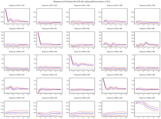
Figure 4.
Results of impulse response function for five liquidity dimensions. Note: The solid blue line represents the median response while the dashed red lines represent upper and lower bounds of the 95% confidence intervals.
Furthermore, this study performs the dependent samples t-test to assess liquidity difference between day session trading and night session trading for the period from 27 September 2021 until 30 December 2022. Table 6 presents a liquidity comparison of the USD Futures market during the day session and night session. When measuring market tightness by effective bid-ask spread, the absolute t-value and the corresponding p-value are 4.2313 and 0.0000, respectively, meaning that there is a difference between market tightness of day session trading and night session trading at 1% significance level. The average value of effective bid-ask spread decreases from 0.2811 (day session trading) to 0.2042 (night session trading). The results show the presence of lower tightness indicating higher transaction costs in day session trading than in night session trading. However, market depth and breadth are stronger in day session trading than in night session trading. When considering market depth by trading volume, the absolute t-value and the corresponding p-value are 15.5539 and 0.0000, respectively, meaning that we can reject the null hypothesis of no difference between market depth of day session trading and night session trading at 1% significance level. The average trading volume is 24,105 contracts per day in day session, and it decreases to almost half of the volume in the night session. When considering market breadth by the Amihud illiquidity ratio, the absolute t-value and the corresponding p-value are 9.3409 and 0.0000, respectively, meaning that we can reject the null hypothesis of no difference between market breadth of day session trading and night session trading at 1% significance level. The average value increases from 0.5974 (day session trading) to 1.4637 (night session trading). A deeper and broader market in day session trading emerges, because of the availability of a large number of orders and the ability of the market to have smoother trading in day session trading than in night session trading. Additionally, there are no differences in terms of market immediacy and market resiliency between day session trading and night session trading. When measuring market immediacy by coefficient of elasticity of trading, the absolute t-value and the corresponding p-value are 0.7800 and 0.4360, respectively, meaning that we cannot reject the null hypothesis of no difference between market immediacy of day session trading and night session trading. There is no difference in the speed of execution during day and night session trading. The results also show that when measuring market resiliency by the market efficiency coefficient, the absolute t-value and the corresponding p-value are 0.1254 and 0.9003, meaning that we cannot reject the null hypothesis of no difference between the USD Futures’ market resiliency of day session trading and night session trading.
Table 6.
Comparison results of USD Futures between day and night sessions for five liquidity dimensions.
5. Conclusions
USD Futures have been traded in the Thailand Futures Exchange (TFEX) since 27 September 2021. Over the past three years, USD Futures have shown significant growth due to exchange rate fluctuations. Since 27 September 2021 onwards, the TFEX has added a night session for trading USD Futures, starting from 6:50 p.m.–11:55 p.m. The launch of the night session enables investors to manage their foreign exchange risk more efficiently and to combine USD Futures and foreign assets trading. Therefore, this study aims to analyze the effect of extended trading hours on liquidity in the USD Futures market and to make a comparison of liquidity between day session trading and night session trading.
Using daily data from 2 January 2020 to 30 December 2022, this study develops a Vector Autoregression model of order 5 (VAR(5)) to examine the simultaneous relationships among five liquidity dimensions, namely tightness, depth, breadth, immediacy, and resiliency. By adding the dummy variable into VAR(5) to capture the effect of night session introduction on market liquidity, the empirical results show that market depth and breadth are even stronger after a longer trading session. These results are in confirmation to those obtained by Jiang et al. (2020) in the SHFE gold and silver futures market. Further, it is evident that the current values of all liquidity measures are positively dependent on one or two days of own lagged values. All liquidity measures also respond quickly to their own lagged changes, confirming the results obtained by Naik et al. (2020) in the Indian equity market. Using the Granger causality test, market tightness and market breadth are interdependent. While market breadth and market resiliency are both statistically useful in forecasting market immediacy, market immediacy only shows the impact on market resiliency. Market depth is not useful in forecasting other liquidity dimensions. This study also conducts the dependent samples t-test to assess liquidity difference between day session trading and night session trading using daily data from 27 September 2021 to 30 December 2022. The results show the presence of lower tightness in day session trading than in night session trading. These empirical results are generally in line with those of gold and silver futures in China (see Jiang et al. 2020). However, market depth and breadth are stronger in day session trading than in night session trading because of the availability of a large number of orders and the ability of the market to have smoother trading in day session trading than in night session trading.
Therefore, the TFEX should consider a longer night session in line with other global futures markets due to the positive effect of extended trading hours on market depth and breadth. Moreover, night traders should be aware of liquidity risk due to low night session trading volume. The TFEX should lower its night trading fees and conduct public relation activities to bring additional liquidity in the night session. For future research, the current study can be extended by providing a more comprehensive analysis of night session characteristics and a detailed cause of the liquidity problem during night session trading.
Funding
This research was funded by Department of Economics, Faculty of Economics, Kasetsart University.
Data Availability Statement
The data can be made available on reasonable request to the author.
Conflicts of Interest
The author declares no conflict of interest.
References
- Amihud, Yakov. 2002. Illiquidity and Stock Returns: Cross-Section and Time-Series Effects. Journal of Financial Markets 5: 31–56. [Google Scholar] [CrossRef]
- Basirian, Elnaz, and Mohammad Hadi Sehatpour. 2021. Study of Factors Affecting the Liquidity of Futures Contracts, Regarding Order-Based Criteria. Journal of Contemporary Issues in Business and Government 27: 2444–54. Available online: https://cibgp.com/uploads/paper/bbd64a5514644f4a248730d2d3e73c8e.pdf (accessed on 19 June 2023).
- Broto, Carmen, and Matías Lamas. 2016. Measuring Market Liquidity in US Fixed Income Markets: A New Synthetic Indicator. Banco de Espana Working Paper No. 1608. Madrid: Banco de Espana. [Google Scholar] [CrossRef]
- Broto, Carmen, and Matías Lamas. 2020. Is Market Liquidity Less Resilient after the Financial Crisis? Evidence for US Treasuries. Economic Modelling 93: 217–29. [Google Scholar] [CrossRef] [PubMed]
- Corwin, Shane A., and Paul Schultz. 2012. A Simple Way to Estimate Bid-Ask Spreads from Daily High and Low Prices. Journal of Finance 67: 719–60. [Google Scholar] [CrossRef]
- Datar, M. K. 2000. Stock Market Liquidity: Measurement and Implications. Paper present at the Fourth Capital Market Conference, Mumbai, India; Available online: https://www.researchgate.net/profile/Maurice-Ekpenyong/post/What_is_the_valid_instrument_for_stock_prices/attachment/5c6d1c6ecfe4a781a58189f7/AS%3A728312225755140%401550654574221/download/Stock+market.pdf (accessed on 8 August 2023).
- Díaz, Antonio, and Ana Escribano. 2020. Measuring the Multi-Faceted Dimension of Liquidity in Financial Markets: A Literature Review. Research in International Business and Finance 51: 1–16. [Google Scholar] [CrossRef]
- Fett, Nicholas, and Richard Haynes. 2017. Liquidity in Select Futures Markets. White Paper. Washington, DC: Office of the Chief Economist, United States Commodity Futures Trading Commission. [Google Scholar]
- Fung, Hung-Gay, Liuqing Mai, and Lin Zhao. 2016. The Effect of Nighttime Trading of Futures Markets on Information Flows: Evidence from China. China Finance and Economic Review 4: 1–16. [Google Scholar] [CrossRef]
- Hasbrouck, Joel, and Robert A. Schwartz. 1988. Liquidity and Execution Costs in Equity Markets. Journal of Portfolio Management 14: 10–16. [Google Scholar] [CrossRef]
- Jiang, Ying, Neil Kellard, and Xiaoquan Liu. 2020. Night Trading and Market Quality: Evidence from Chinese and US Precious Metal Futures Markets. Journal of Futures Markets 40: 1486–507. [Google Scholar] [CrossRef]
- Klein, Tony, and Neda Todorova. 2021. Night Trading with Futures in China: The Case of Aluminum and Copper. Resources Policy 73: 102205. [Google Scholar] [CrossRef]
- Le, Huong, and Andros Gregoriou. 2020. How Do You Capture Liquidity? A Review of the Literature on Low-Frequency Stock Liquidity. Journal of Economic Surveys 34: 1170–86. [Google Scholar] [CrossRef]
- Naik, Priyanka, B. G. Poornima, and Yeruva Venkata Ramana Reddy. 2020. Measuring Liquidity in Indian Stock Market: A Dimensional Perspective. PLoS ONE 15: e0238718. [Google Scholar] [CrossRef] [PubMed]
- Panagiotou, Panagiotis, Xu Jiang, and Angel Gavilan. 2022. The Determinants of Liquidity Commonality in the Euro-Area Sovereign Bond Market. The European Journal of Finance 29: 1144–86. [Google Scholar] [CrossRef]
- Ripple, Ronald D., and Imad A. Moosa. 2009. The Effect of Maturity, Trading Volume, and Open Interest on Crude Oil Futures Price Range-Based Volatility. Global Finance Journal 20: 209–19. [Google Scholar] [CrossRef]
- Roll, Richard. 1984. A Simple Implicit Measure of the Effective Bid-Ask Spread in an Efficient Market. Journal of Finance 39: 1127–39. [Google Scholar] [CrossRef]
- Sarr, Abdourahmane, and Tonny Lybek. 2002. Measuring Liquidity in Financial Markets. IMF Working Papers 02/232. Available online: https://www.imf.org/-/media/Websites/IMF/imported-full-text-pdf/external/pubs/ft/wp/2002/_wp02232.ashx (accessed on 1 November 2022).
- Trebbi, Francesco, and Kairong Xiao. 2019. Regulation and Market Liquidity. Management Science 65: 1949–68. [Google Scholar] [CrossRef]
- Wang, Jian-Xin. 2010. A Multi-Factor Measure for Cross-Market Liquidity Commonality. ADB Economics Working Paper Series No. 230; Available online: https://www.adb.org/sites/default/files/publication/28274/economics-wp230.pdf (accessed on 1 November 2022).
- Wanzala, Richard Wamalwa. 2018. Estimation of Market Immediacy by Coefficient of Elasticity of Trading Three Approach. Journal of Finance and Data Science 4: 139–56. [Google Scholar] [CrossRef]
- Woo, Mincheol, and Meong Ae Kim. 2021. The Market Impact of Futures Trading by the National Pension Service (NPS) of Korea. Journal of Derivatives and Quantitative Studies 29: 215–33. [Google Scholar] [CrossRef]
- Xie, Linyin, Yuanqing Jin, and Chanxuan Mo. 2022. Predictive and Contemporaneous Power of the Determinants of Stock Liquidity. Front. Psychol 13: 912159. [Google Scholar] [CrossRef] [PubMed]
- Yao, Xuan, Xiaofeng Hui, and Kaican Kang. 2021. Can Night Trading Sessions Improve Forecasting Performance of Gold Futures’ Volatility in China? Journal of Forecasting 40: 849–60. [Google Scholar] [CrossRef]
Disclaimer/Publisher’s Note: The statements, opinions and data contained in all publications are solely those of the individual author(s) and contributor(s) and not of MDPI and/or the editor(s). MDPI and/or the editor(s) disclaim responsibility for any injury to people or property resulting from any ideas, methods, instructions or products referred to in the content. |
© 2023 by the author. Licensee MDPI, Basel, Switzerland. This article is an open access article distributed under the terms and conditions of the Creative Commons Attribution (CC BY) license (https://creativecommons.org/licenses/by/4.0/).