Market Quality and Short-Selling Ban during the COVID-19 Pandemic: A High-Frequency Data Approach

Abstract

The recent emergence of COVID-19 and the subsequent short-selling restriction (SSR) imposed on some equity markets provide us with a unique framework to analyze the effects of this kind of measure on market quality in the context of increasingly automated equity markets. We contribute to the literature by analyzing the microstructure and quality parameters of the Spanish equity market during COVID-19 and SSR. We study four subperiods, namely pre-crisis, turmoil, SSR, and first de-escalation periods, by means of a tick-by-tick dataset and the complete limit order book (LOB). We observe the following impact of the SSR on the constituents of IBEX 35: (1) the SSR did comply partially with its aim at an intraday level regarding volatility, but liquidity was reduced; (2) liquidity deterioration affected more the sell than the buy side of the LOB; (3) high-frequency activity (HFT) diminished during SSR, reinforcing volatility; (4) negative effects on liquidity and HFT diminished and disappeared as the ban was lifted; (5) HFT unidirectionally Granger causes 1 min realized volatility while the natural logarithm of the slope of the LOB bidirectionally Granger causes 1 min realized volatility.

1. Introduction

The prevalence of algorithmic trading (AT), and high-frequency activity (HFT) in particular, has increased significantly in recent years (Baron et al. 2019; Borch 2016; Cvitanic and Kirilenko 2012; Dall’Amico et al. 2019; Golub et al. 2012; Hasbrouck and Saar 2013; Jovanovic and Menkveld 2012). Financial literature has thoroughly studied market quality parameters and their relationship with AT and HFT, although inconclusive findings have been reached regarding volatility, liquidity, price efficiency, and transaction costs related to HFT’s impact and behavior (Virgilio 2019). If one conclusion can be drawn it is that technology and new AT and HFT trading strategies significantly affect market microstructure (O’Hara 2015). This paper aims to jointly analyze the main quality parameters of the constituents of the Spanish equity index IBEX 35 and relate them to changes in the microstructure in several market situations at a high-frequency level of activity.

MiFID II clearly establishes what can be considered AT and HFT in a market. Specifically, AT is described as “trading in financial instruments where a computer algorithm automatically determines individual parameters of orders such as whether to initiate the order, the timing, price or quantity of the order or how to manage the order after its submission, with limited or no human intervention, and does not include any system that is only used for the purpose of routing orders to one or more trading venues or for the processing of orders involving no determination of any trading parameters or for the confirmation of orders or the post-trade processing of executed transactions” (Article 4(1)(39) of MiFID II), while HFT is defined as “an AT technique characterized by: (a) infrastructure intended to minimize network and other types of latencies, including at least one of the following facilities for algorithmic order entry: co-location, proximity hosting or high-speed direct electronic access; (b) system-determination of order initiation, generation, routing or execution without human intervention for individual trades or orders; and (c) high message intraday rates which constitute orders, quotes or cancellations” (Article 4(1)(40) of MiFID II).

The turmoil in the financial markets created by the COVID-19 shock is a unique opportunity to analyze the effects of interventionist policy measures over said market quality parameters in the context of increasingly automated markets. During the first wave of the COVID-19 crisis, the European Securities Market Authority (ESMA) prompted six European authorities to ban short selling in the most liquid shares. In Spain, Comisión Nacional del Mercado de Valores (CNMV) imposed the prohibition of short selling over liquid stocks on 17 March 2020 in accordance with Articles 23 and 24 of Regulation (EU) No. 236/2012 of the Short Selling Regulation in those inventories that involve the creation or increase of a net short position on the Spanish shares admitted to trading in the Spanish trading venues. The decision was implemented due to “extreme volatility taking hold of European securities markets, including those based in Spain, their performance in the context of the situation arisen as a result of the virus COVID-19 and the risk of disorderly trading taking place in the following weeks”. On 17 March 2020, a proposed emergency measure introduced by CNMV under Articles 20(2)(a) and (b) of Regulation (EU) No. 236/2012 (ESMA70-155-9556), subsequently imposed long-term exchange-wide short-selling ban effects, which started on 18 March 2020 and was lifted on 18 May 2020 as market conditions improved. Short selling adds liquidity and benefits price discovery (Massa et al. 2015; Sobaci et al. 2014; Feng and Chan 2016; Wang et al. 2017). However, it is still controversial if these restrictions with naked short selling actually reduce financial risks, through the reduction of the volatility of returns, introducing factual confidence in markets.

The period of exogenous shock due to COVID-19 and the ban on short selling in the Spanish stock market is an eligible one to analyze the impact of these kinds of measures on market quality and to assess whether the ban complied with its objectives or not. The increased prevalence of AT and HFT and their impact on market microstructure make it necessary to revisit the consequences of short-selling restrictions, since previous results may not be valid in current markets. Although the Spanish equity market is still not labeled as an HFT venue, it provides low-latency infrastructures, co-location services, and direct access to algorithms, which make it a suitable place to study the effects of SSR on market microstructure and quality in the context of modern, highly automated markets.

The main aim of this paper is to analyze different market quality measures and the prevalence of HFT on the IBEX 35 constituents during four different subperiods: the pre-pandemic period, the initial market turmoil due to the COVID-19 pandemic, the short-selling ban window, and, finally, the first phase of de-escalation. We contribute to the literature by analyzing the microstructure and quality parameters of the Spanish equity market during the emergence of COVID-19 and the subsequent SSR by means of a unique dataset including tick-by-tick changes in the LOB. The data, containing twenty levels of the positions of the LOB, allow the detection of the changes at the microstructure level and shed some light on the impact generated by SSR with low-latency infrastructures and co-location services. Buy, sell, modify, and cancellation orders arriving at the LOB can be perfectly linked to executed trades. Proxies based on message traffic have been used to identify AT and HFT by academics, industry bodies, trading venues, and regulators. We use the number of messages per EUR 100 of trading volume along with message-to-trade ratios as a proxy of high-frequency activity (Hendershott et al. 2011). We revisit liquidity measures, price efficiency, and volatility. Finally, we test for panel data Granger causality between realized 1 min volatility with a high-frequency proxy and the natural logarithm of the slope of the LOB.

More precisely, we provide research on a tick-by-tick basis about the message flow in the Spanish market from the pre-pandemic period to the first stage of de-escalation. Specifically, this paper identifies (1) the prevalence of high-frequency activity with indirect approaches such as message-to-trade ratios, messages per second, and changes in the midpoint price different from zero (Bouveret et al. 2014) and (2) changes in market quality across COVID-19 periods, either before or after the SSR, from 18th of March to 18th of May 2020; finally, (3) we analyze whether short sellers act as essential information intermediaries enhancing the information environment in normal and “extreme” times, as pointed out by Marsh and Payne (2012) in relation to the 2008 financial crisis, studying whether short-selling restriction impacts the symmetric deterioration of the elasticity of the LOB. Therefore, we formulate the following hypotheses:

Hypothesis 1.

The effectiveness of short sale constraints in reducing extreme volatility is low, consistent with most previous literature.

Hypothesis 2.

Market quality deteriorated during the SSR period.

Hypothesis 3.

Short-selling bans drastically reduce high-frequency activity, based on Granger causality.

Hypothesis 4.

Deterioration was non-symmetric in the ban period; it was worse on the sell side of the LOB.

Hypothesis 5.

High-frequency activity and the slope of the LOB Granger cause realized volatility.

HFT prevalence features are, among others, (1) the low–zero inventory at the end of the day in HFT firms; (2) the smaller size per trade, as pointed out by Menkveld (2013); (3) the existence of co-location services or low-latency infrastructures; and (4) high message traffic per trade and per order. Extant HFT literature bases proxies on message traffic, which should be increased if HFT increases (Hendershott et al. 2011). Specifically, these types of measures were used as indirect proxies by Brogaard et al. (2015, 2017), Boehmer et al. (2018), Brogaard et al. (2013), and Friederich and Payne (2012, 2015).

The interaction between high message ratios mainly due to HFT has affected microstructure parameters at the intraday level compared to a daily basis. Brogaard et al. (2019) concluded that more limit orders were associated with better price discovery but more volatility and adverse selection costs. This should be considered due to the partial impact explained by high-frequency activity. Due to the expansion of AT and high-frequency AT (HFT), MiFID II/MiFIR imposes certain obligations on trading venues to protect the integrity and quality of the market. Co-location services, market-maker activities, capacity and resilience of systems, and order-to-trade ratio are some of those. Trading venues are required to have systems that allow the limitation of the proportion of unexecuted orders that can be entered into the system by each participant. In the case of the Spanish stock market, the entry into force of the MiFID II directive on 1 January 2018 meant that it was no longer mandatory to reveal the broker code behind each order. Therefore, no detailed information about the companies that operate or participate in high-frequency trading as their main line of business is available from the market. However, a low-frequency infrastructure (SMART SIBE) was established in 2012. Although no member was registered as an HFT proprietary business, since 16 April 2012, the latency dropped to less than 1 millisecond. The ESMA Economic Report (Bouveret et al. 2014) presented an overview of HFT from different approaches, such as HFT flags and lifetime orders, in which the Spanish stock market had 20% of the value traded by HFT back in 2013, according to the latter, although no HFT-flag was available. Investment banks’ activity was 59% of the total value traded, of which 22% was HFT. In terms of the number of trades (orders), their activity accounted for 62% (70%) of the total number, of which 20% (27%) was HFT.

With regard to the private information behind Spanish HFTs and ATs, it seems appropriate to specify that algorithmic trading orders are usually based on the evolution of market parameters, more than on the information leakage related to macroeconomic fundamentals. These are orders that do not need to be managed by the broker; on the contrary, it is the system itself that is responsible for managing them internally, according to the algorithm and the parameters chosen by the trader. Without intending to present an exhaustive list, some typical variables included in the algorithms are the following: volume-weighted average price (VWAP), time-weighted average price (TWAP), percent of volume (POV), SOR best price, and SOR max volume.

Huhtilainen (2017) and Losada López and Martínez (2020) pointed out that banning short selling is not an effective tool (or at least it is limited) for containing extreme price volatility, improving liquidity (bid–ask spread), and obtaining better results in the Amihud illiquidity ratio. Diamond and Verrecchia (1987) find that short sellers are informed traders that provide price efficiency, so prohibiting their activity will potentially prevent information from reaching the market. However, the former loss of depth is not significantly due to the ban rather than to country premia, on a daily basis. Our results indicate that the Amihud ratio throws greater coefficients on a trade-by-trade basis, and it is not significant due to the SSR period. Our results are consistent with prior theoretical and empirical work (European Securities and Markets Authority 2022), as the COVID-19 short-selling bans are associated with more pronounced liquidity deterioration on large stocks.

According to Brogaard et al. (2017), liquidity and price efficiency improved due to low-frequency trading during the 2008 short-selling ban, and they deteriorated because of high-frequency trading due to unfavorable selection of limit orders, avoiding low-frequency trading in periods of short-selling restrictions. We emphasize that high-frequency messages by trade (our proxy for HFT) decreased significantly during SSR on the venue, but liquidity did not improve relative to the rest of the periods. Losada López and Martínez (2020), in accordance with the main strand of the literature, find that the SSR had a very negative impact on bid–ask spreads and depth in IBEX 35 constituents, but the Amihud illiquidity ratio is not significantly due to the ban. Siciliano and Ventoruzzo (2020), on the other hand, assert that liquidity (spread and Amihud illiquidity ratio) deteriorated with the ban in 2020. Regarding the provision of liquidity in the market in a high-frequency world, there is a branch of the literature focused on the measurement of order flow toxicity (the expected loss from trading against better-informed counterparties) headed by the papers by Easley et al. (2012) and their VPIN measure. According to these authors, providing liquidity in an HF environment introduces new risks: when order flows are balanced, HF traders earn tiny margins on massive numbers of trades, but when order flows become unbalanced, they face the prospect of losses due to adverse selection. Therefore, order flow toxicity can cause market makers to leave the market, triggering illiquidity. However, the accuracy of the VPIN measure as an estimator of toxicity has been questioned by Andersen and Bondarenko (2014a, 2014b, 2015), although these papers have been subsequently refuted in turn by Easley et al. (2014). This debate about the measurement of the existing risk does not erase the fact itself that order toxicity (as measured by the existence of imbalances in the LOB) can lead to a notable decrease in liquidity. Recently, the VPIN measure has been also used to assess whether HFTs are responsible for extreme price movements, and it was observed that they reduce their trading prior to price jumps, while low-frequency traders remain as the main market participants when jumps take place (Prodromou and Westerholm 2022). Informed trading has been the object of study in the FX market, where it has been observed that there is a certain intraday momentum effect due in part to informed investors (Gençay and Gradojevic 2013), who, in order not to reveal their positions, could concentrate their trades at the times of greatest volume (usually the opening and the closing, due to the well-known U-shape in intraday trading volume) (Elaut et al. 2018). These studies have been replicated in the S&P500, and it was concluded that the intraday momentum effect holds (Gao et al. 2018) but disappears during the COVID-19 pandemic shock (Hossain et al. 2021). However, on the one hand, the conclusions of FX studies are not 100% applicable to stock markets given the special characteristics of the former (trading is more decentralized and opaquer in the FX market, and trades can occur around the clock as opposed to fixed opening and closing hours, as indicated by D’Souza (2007)). On the other hand, although all HFT trading is sometimes considered to be informed, there are different levels of informativeness, as Benos and Sagade (2016) pointed out: high-frequency traders who pursue strategies that require the use of aggressive trades are most informed, as opposed to passive high-frequency traders who more likely act as market makers.

Price efficiency in this pandemic crisis could be treated in a different context compared to other short-sales restrictions due to suggested disinformation or incomplete information, even in efficient markets, since the situation of a new disease that generates a global pandemic reduces the real information and its incorporation, worsening the price efficiency, according to the European Securities and Markets Authority of 15 April 2020.

With regard to the symmetry of the impact of short-selling restriction (SSR) over the buy and the sell sides of the LOB, Marsh and Payne (2012) found that the impairment was symmetrical to financial stocks, affecting the buy and sell sides of the order book equally during the 2008/2009 financial crisis in the UK, while Duong and Kalev (2007) found that the buy side of the LOB is more informative than the sell side. Our results reflect a more dispersed (concentrated) order quantity in the sell (buy) side of the LOB during the short-selling restriction period, stronger in small companies than in large capitalization stocks. Consistent with Duong and Kalev (2007) we find dispersion of beliefs about asset values and the slope of the buy side of the book looks more informative than the sell side (Pascual and Veredas 2006).

The slope of the LOB, raised by Næs and Skjeltorp (2006), describes how the quantity supplied in the order book changes as a function of prices. This measure relates depth with the number of orders and quantity on both sides of the LOB. According to the authors, the flatter (steeper) the slope, the more widely distributed (concentrated) the volumes in the order book are. In addition, the volatility–volume relationship (negative related to slope) increases due to the dispersion of beliefs partially informed by the slope of the LOB. In addition, the authors claim that this measure has an informative influence as an endogenous variable explaining volume, trades, and price autocorrelation. Duong and Kalev (2007) found that the slope of the buy side of the LOB is more informative compared to the sell side of the LOB in the Australian Stock Exchange (ASX). The slope of the LOB considers the average of the slopes on the demand and supply sides. We approach this relationship from the point of view of comparing both slopes (demand and supply) as a ratio in each period. Goldstein and Kavajecz (2004) evidenced a negative relation between the shape of the LOB and volatility in the NYSE during the October 1997 turbulent period.

The remainder of the paper is organized as follows: Section 2 presents extant literature on market quality and the effects of the COVID-19 pandemic shock; Section 3 describes the data and the measures applied in the research; Section 4 presents the main results obtained; finally, Section 5 concludes.

2. Literature Review

The COVID-19 pandemic has had a great impact, affecting practically all sectors, levels of society, and countries in the world. This pandemic has developed very differently from previous health threats, having spread rapidly until it was declared a global pandemic in mid-March 2020. Government attempts to counteract the effects of the pandemic have included measures to limit the severe impacts of COVID-19 throughout the world, the most striking being lockdowns, but without forgetting other movement restrictions, including learning from home or working from home for non-essential businesses or services, as well as banning crowds and establishing fiscal stimulus.

The fact that it is a relatively recent shock has not been an obstacle to the generation of a plethora of research papers focused on this period; however, the literature is still limited since there are several questions yet to be identified and explored on the financial effects of the COVID-19 pandemic. In this literature review, we are going to focus on those papers whose scope is the impact of the shock caused by the pandemic on market efficiency. For an extensive and systematic review of the early literature on the impact of COVID-19 on markets, see the work of Anggraini et al. (2022).

With respect to liquidity, mixed results have been obtained when analyzing what happened in different markets. On the one hand, most of the studies have detected a worsening of liquidity measures in practically all the markets under analysis: for example, Haroon and Rizvi (2020), using a sample of emerging markets, find that an increase in the number of confirmed coronavirus cases is associated with deteriorating liquidity in financial markets. Foley et al. (2022), using data from North America, Europe, and Australia, claim that there are negative liquidity impacts most pronounced for stocks most exposed to HFT market makers. However, Chakrabarty and Pascual (2022) observe a drop in liquidity in assets belonging to the S&P500, although less pronounced in those assets more actively traded by AT. Other papers pointing in this direction are those of Damien (2021), Tissaoui et al. (2021), and Priscilla et al. (2022). On the other hand, authors such as Marozva and Magwedere (2021) have observed an improvement in liquidity in the capital market, with a negative relationship between illiquidity measures and COVID-19, more prevalent in developed markets than in emerging ones.

The recent pandemic also had a negative effect on volatility in the market. Research papers around the world show an increase in volatility coinciding with the outbreak of the pandemic (Ali et al. 2020; Barro et al. 2022; Chowdhury et al. 2021; David et al. 2020; Mishra and Mishra 2021; Sheraz and Nasir 2021; Uddin et al. 2021). Gao et al. (2021) find that the impact of COVID-19 on the stock market showed a significant leverage effect in both the US and China, imposing a stronger effect on the stock market volatility when it was already high. Engelhardt et al. (2020) note that, in spite of the negative impact of the pandemic, stock markets’ volatility is significantly lower in high-trust countries. Some studies have tried to identify the origin of this volatility, focusing on factors such as the dissemination of news about the health crisis (Alzyadat et al. 2021; Mishra and Mishra 2021), activities that facilitate mobility and economic shocks (Egger and Zhu 2021), fear (Li et al. 2021), and the implementation of mobility restriction measures (Chowdhury et al. 2021; Hunjra et al. 2021). Ftiti et al. (2021) also found that market sentiment toward the pandemic had significant effects on stock price volatility.

The impact of the pandemic could be summed up in a notable decrease in market efficiency, as pointed out by authors such as Dias et al. (2020), Hong et al. (2021), and Ozkan (2021). Our paper contributes to the existing literature by uncovering the information buried in the intraday data about the changes in market quality in various subperiods (including a short-selling ban), through the application of relevant measures and taking into account the activity of HFT and AT.

3. Materials and Methods

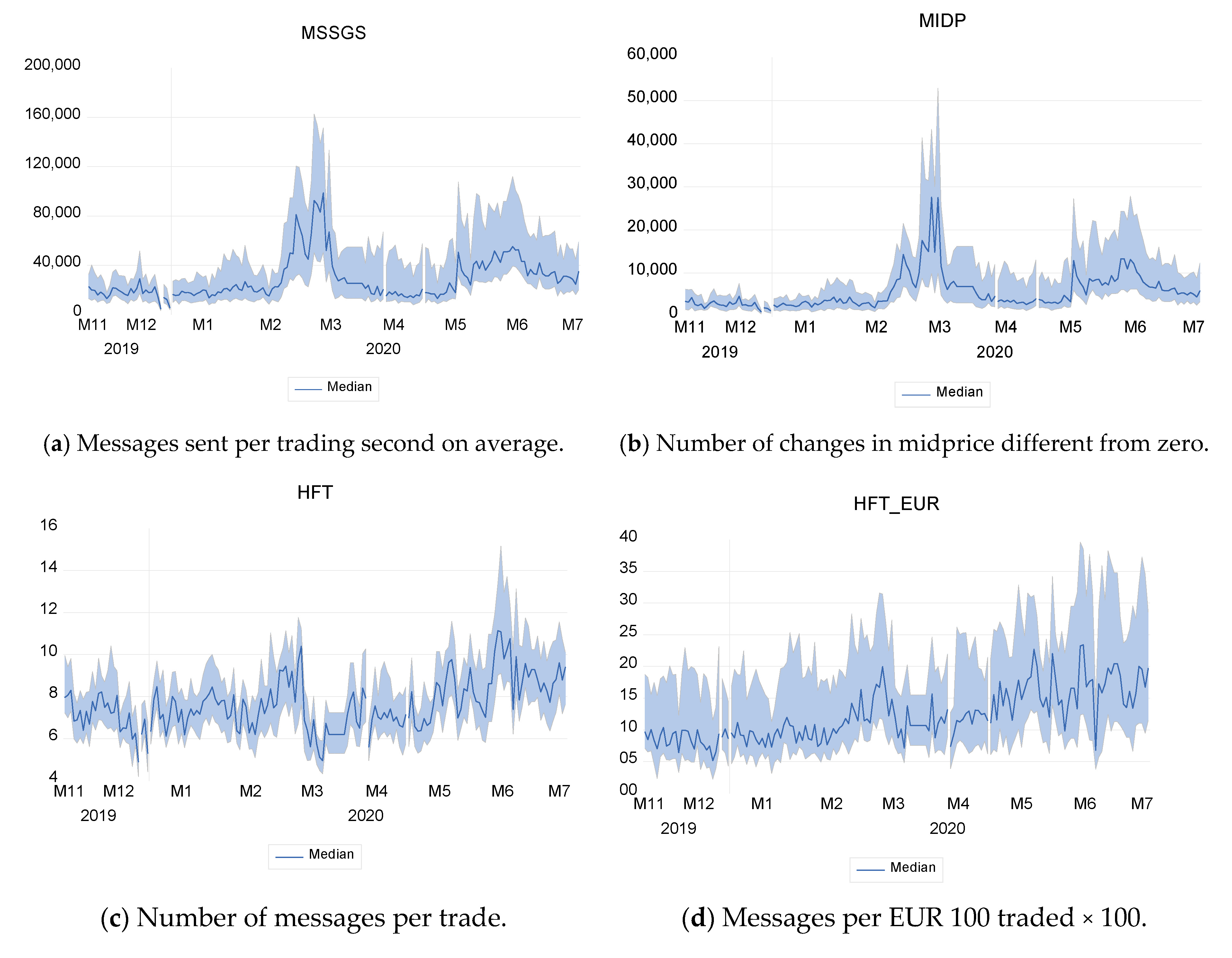
For conducting the research shown in this paper, tick-by-tick databases are used, containing both messages from the LOB and data on the transactions of ordinary shares traded on the electronic platform of the Spanish market. The original data have been supplied by BME Market Data. The analysis period covers 184 days, divided into four time-windows: pre-pandemic (W0), from 20 November 2019 to 20 January 2020; pandemic crash (W1), from 21 January 2020 to 17 March 2020; short-selling ban (W2), from 18 March 2020 to 18 May 2020; and de-escalation (W3), from 19 May 2020 to 13 July 2020. The temporary ban on short sales concerning the 13th of March is considered partial and not included in the period because it was not extensively informed further than that day. The sample consists of 35 stocks that are constituents of IBEX 35, subdivided into quartiles by market capitalization on 19 December 2019.

The LOB data, provided by BME DATA FEED Services, include the twenty best quotes, both bidding and asking, which are updated every time a new message is sent to the market (i.e., a limit order, a market order, a cancellation, or an order modification). For each level of the LOB and for each stock, there is information about the quotes, the number of visible orders at each quote level, and the depth. Each executed trade can be perfectly joined with the limit book order messages and changes. A unique sequence number is generated every time a buy, sell, cancellation, or modification order message reaches the Spanish Stock Exchange Interconnection System (SIBE), allowing us to have a snapshot of the LOB every time it is updated with a message. In this way, we relate the number of messages arriving at the SIBE to each executed trade. No information about hidden depth and iceberg orders is available in the data. Because the first and last minutes are key for our study, all messages and order data from the pre-auction and auction periods have been included in the study.

Group 1 measures: algorithmic data and high-frequency trading proxies.

An accurate identification of HFT presence is challenging to achieve; no unique or easy method can accurately estimate the percentage of HFT, apart from, of course, labeled data. Since the implementation of MiFID II in 2018, BME DATA FEED Services provides detailed information about the LOB and transactions, but it does not include HFT labels in the data. However, another label (AlgorithmicTradeIndicator) reveals whether the trade was submitted by a trading algorithm. In this paper, indirect proxies have been calculated due to the fact that flagged HFT labeled data do not exist in the Spanish market.

Regarding some indirect HFT metrics, we consider, as MIFID II further defines under Article 19 of Commission Delegated Regulation (EU) 2017/565, high message intraday rate “as the submission, on average, of any of the following: “(a) at least 2 messages per second with respect to any single financial instrument traded on a trading venue; (b) at least 4 messages per second with respect to all financial instruments traded on a trading venue; where only messages concerning financial instruments for which there is a liquid market are to be included in the calculation”. The limit is defined at firm activity, so as we do not have broker’s data, we will analyze changes in the number of messages per second and per executed trade over periods as in previous literature.

Infrastructure requirements were implemented in the Spanish stock venue in 2012 with the Smart SIBE, which complies with one of the HFT and AT requirements, which is using co-location and proximity services to minimize latency. At a microstructure level, high-frequency data, message traffic flow, and message-to-trade ratios are fundamental to include in the Spanish market quality study. We have to highlight that these high-frequency activity proxies cannot be taken purely as an indicator of HFT, although the imprint of this activity on said measures is definitely observable. We analyze changes in average trade size, messages sent per second, messages per trade, midprice changes on the LOB, and number of trades. Additionally, we use the Hendershott et al. (2011) combined number of messages per EUR 100 of trading volume along with message-to-trade ratios as an indirect approach to HFT. In all the cases, high-frequency activity increases these measures and vice versa, except in the case of average size, where the prevalence of HFT trades usually reduces the quantity of stocks in each trade.

Firms generating message traffic of more than two messages per second or 75,000 messages per trading day are HFT firms if they also fulfill the other criteria of the HFT act. Jovanovic and Menkveld (2012) define HFT firms as intermediaries with high volume traded and near-to-zero intraday and overnight inventories. As it is not mandatory to disclose the broker code, the average end-of-the-day inventories of brokers can not be calculated. The measures presented below are indirect proxies for high-frequency activity, which are calculated per transaction and on a tick-by-tick basis with LOB messages. Then, they are averaged by asset and day to obtain daily series that cover the entire analysis period. We have contrasted non-normal distribution medians of algorithm trading, average size per trade, messages per second, midprice changes different from zero, number of executed trades, and number of messages per EUR 100 traded on the complete LOB. These measures are defined in Equations (1)–(6).

$$ALGO\_T{R}_i=100 \times {\left(orders submitted by a trading algorithm/orders submitted\right)}_i$$

(1)

$$AVGSIZE={(Traded volume/\#Executed trades)}_i$$

(2)

$$MESSAGES\_SE{C}_i={(\#messages sent to LOB/\#seconds of trading day)}_i$$

(3)

$$MESSAGE{S}_{TRADE}{\left(HFT\right)}_i={(\#messages sent to LOB/\#trades)}_i$$

(4)

$$MIDPRICE\_CHANGE{S}_i={\left(\#changes in midpoint price different of zero\right)}_i$$

(5)

$$MESSAGES\_€{100}_i=\#messages sent to LOB/100 euro traded$$

(6)

Group 2 measures: liquidity measures.

Market quality measures revisited in this paper are calculated on an intraday basis. Liquidity is one of the most important market parameters (Ma et al. 2018). The measures considered at an intraday, high frequency, level include direct and indirect approaches used in the literature: average volume as the daily traded volume, bid–ask spread calculated as the difference between the best buy price and the best-selling price over the midpoint, relative spread as spread divided by midpoint price, and depth (as the average between the accumulated stocks at the twenty best buy and sell prices). We also obtain liquidity measures such as the Amihud illiquidity ratio on a trade-by-trade basis. The liquidity measures taken into account are shown in Equations (7)–(10).

$$AVGVO{L}_i=Average traded volume in a da{y}_i$$

(7)

$$SPREA{D}_i=Best ask pric{e}_i-Best bid pric{e}_i$$

(8)

$$RELATIVE SPREA{D}_i=2 x SPREAD{ }_i/\left(Best ask pric{e}_i+Best bid pric{e}_i\right)$$

(9)

$$Dept{h}_i=(Accumulated ask orders \left(20 levels\right){ }_i+Accumulated bid orders {\left(20 levels\right)}_i)/2$$

(10)

We have calculated the Amihud (2002) illiquidity measure, adapting from daily to trade-by-trade level, as the ratio of absolute stock trade-by-trade return to the volume in EUR obtained from each trade. The original Amihud illiquidity measure is calculated on a daily basis, comparing close to the previous day close to calculate the absolute return compared to the volume in USD. It is not necessary to apply revision due to the case of a trade-by-trade basis, as open price and prior-close price are coincident (Barardehi et al. 2020). The mean of the daily data of each stock is used as input for the constituents of the quartile-period panel. For the rest of the test, the average across IBEX 35 constituents is used.

$$AMIHU{D}_{i,trades}=\frac{1}{N_{trades,i}}{\displaystyle \sum }_{s=1}^{N_{trades}}\left\{\frac{\left|retur{n}_{i,trade}\right|}{€volum{e}_{i,trade}}\right\}$$

(11)

where, at an asset level ($i$), $N_{trades,i}$ is the number of executed trades, $retur{n}_{i,trade}$ is the realized return in each trade, $€volum{e}_{i,trade}$ is the volume in EUR consumed in each trade.

We contrast out average-pairwise verification among stocks, considering the non-normal distribution of data. Non-parametric mean with t-test with two paired samples and median test with ranked signed Wilcoxon verification test (Wilcoxon 1945) is used. Changes between the four periods have been calculated on a tick-by-tick/trade basis; otherwise, frequency has been specified in the labels.

Literature on the EU short-selling restriction period linked to COVID-19 usually measures the bid–ask spread using daily (end of the trading day) data. Therefore, our analysis of the full order book at a high frequency level can provide a deeper insight into liquidity by revealing the depth available for trade at all price levels throughout the day, rather than focusing on just the prices at the top of the book at one specific point in time. The combination of higher frequency data of the LOB, orders, volumes, and prices across the whole LOB, can uncover even more precise liquidity information.

Group 3: volatility and price efficiency measures.

The first of the price efficiency indicators that have been identified is the slope of the LOB. We adapt it to analyze the symmetry in the deterioration on both sides of the order book. We analyze the daily average relation between the ratio of the slope of the demand side and the supply side in the visible order book. We processed each of the steps described in Næs and Skjeltorp (2006) as in Equations (12)–(14).

$$D{E}_{i,t}^S=\frac{1}{N_B}\{\frac{v_1^B}{\raisebox{1ex}{$p_1^B$}\!\left/ \!\raisebox{-1ex}{$p_0^B$}\right.-1}+{\displaystyle \sum }_{t=1}^{N_B}\frac{\raisebox{1ex}{$v_{t+1}^B$}\!\left/ \!\raisebox{-1ex}{$v_t^B$}\right.-1}{\raisebox{1ex}{$p_{t+1}^B$}\!\left/ \!\raisebox{-1ex}{$p_t^B$}\right.-1}\}$$

(12)

$$S{E}_{i,t}^S=\frac{1}{N_A}\{\frac{v_1^A}{\raisebox{1ex}{$p_1^A$}\!\left/ \!\raisebox{-1ex}{$p_0^A$}\right.-1}+{\displaystyle \sum }_{t=1}^{N_B}\frac{\raisebox{1ex}{$v_{t+1}^A$}\!\left/ \!\raisebox{-1ex}{$v_t^A$}\right.-1}{\raisebox{1ex}{$p_{t+1}^A$}\!\left/ \!\raisebox{-1ex}{$p_t^A$}\right.-1}\}$$

(13)

$$SLOP{E}_{i,t}=\frac{1}{N_i}{\displaystyle \sum }_{s=1}^{N_i}\left\{\frac{S{E}_{i,t}^S+D{E}_{i,t}^S}{2}\right\}$$

(14)

where $S{E}_{i,t}^S$ $(D{E}_{i,t}^S)$ is the average slope of the sell (buy) side. N_A (N_B) is the total number of ask (bid) prices or tick levels, containing orders. Let $t=0$ denote the bid–ask midpoint.$p_0^A$ and $p_0^B$ are the bid–ask midpoint, and $t=1$ represents the best quote with volume. Finally, $v_1^{}$ is the natural logarithm of accumulated total share volume at each level $t$.

The average slope of the day is calculated following Equation (15), where $N_i$ is the number of exchanges or snapshots on the LOB for each asset.

$$ELO{B}_{i,t}=\frac{1}{N_i}{\displaystyle \sum }_{s=1}^{N_i}\left\{\frac{D{E}_{i,t}^S}{S{E}_{i,t}^S}\right\}$$

(15)

We present Equation (15) where we estimate the average of the ask side (SE) divided by the average of the bid side (DE) for each snapshot change of the complete LOB and take the daily ratio (ELOB) to compare the slopes of both sides of the LOB. This will highlight the changes between price concentration or dispersion on the ask side compared to those on the bid side, giving us information about the symmetry deterioration or improvement of the limit order book. The novelty of applying these measures using intraday data is of interest because the use of daily data could hinder HFT due to the low–zero inventory of HFT firms at the end of the day.

Regarding volatility, we revisited parameters such as realized volatility at one-minute frequency, realized volatility at 30 min frequency, and price autocorrelation to add consistency to the price efficiency analysis. We calculate realized volatility as the standard deviation of returns for each frequency studied. We have calculated realized volatility of returns for 1 min (RVol_1m) and 30 min (RVol_30 min) periods. If prices were efficient according to the efficient market theory, the 1 min realized volatility scaled to 30 min (multiplying it by $\sqrt{30}$) should be the same as (or close to) 30 min realized volatility, Equation (16). We used the coefficient between 30 min volatility and scaled 1 min volatility as in Equation (16) as an additional price efficiency intraday measure. Again, looking only at daily changes in volatility may hide HFT as was the case in the liquidity measures, so the use of intraday data could be of help to avoid the loss of information.

$$COEF\_VO{L}_{i,t}=\frac{\sqrt{30}·{\sigma }_{1min}}{{\sigma }_{30min}}$$

(16)

$$AUTOCORR=firstorderreturnautocorrelationin1minfrequency$$

(17)

According to price efficiency theories, ideally, this ratio should be around 1, and non-first-order or residual first-order return autocorrelation should exist, reflecting a random walk. The greater the volatility coefficient ($COEF\_VO{L}_{i,t}$) and the first-order return autocorrelation ($AUTOCORR$), the less efficient prices are. In low-frequency data, return or prices are unpredictable, following a random walk. In high-frequency data, Roll (1984) demonstrated that the noise component of prices generates a negative autocorrelation in price changes. We calculate 1 min frequency autocorrelation.

Seasonality in intraday dynamics exists and is well revised in financial literature. Effects on variables under high-frequency data vary depending on the interval chosen. Patterns can be found in the distribution of both intraday returns and main market quality measures such as liquidity and volatility. Autocorrelation or co-movements generate “U”-shaped or inverted “J” patterns as noted by Martens et al. (2002), Hua and Li (2011), and Tian and Guo (2007), among others; Kottaridi et al. (2020) pointed out that the intraday pattern is more pronounced in specific days of the week in the case of returns and volatility. During the COVID-19 period, although the “U”-shape persisted, Kubiczek and Tuszkiewicz (2022) pointed out that private investors operated more, decompensating the usual distribution of the percentages of data during the day that usually exists at the opening and close of the trading day.

These patterns, and also their causes, vary between different markets. In the case of equity markets, Ozenbas (2008) noted that in different regions such as US and EU, changes in the rules (such as call auctions or the extension of trading hours) affect the shape of the distribution. Eaves and Williams (2010) assert that the timing of privately informed traders cannot be the source of intraday patterns in the Tokyo Grain Exchange. Seasonality (both intraday and day-of-the-week), despite being caused by different events, can be observed in the increasing volatility and liquidity in auctions and in the first hours of trading, thus allowing informed investors to use those periods of the day to operate their volumes as indicated by Gençay et al. (2015).

Data can be deseasonalized to focus on the dynamics around average behavior, as in the work of Bińkowski and Lehalle (2018), taking the natural logarithm to symmetrize the distribution and eliminate the seasonal component, thus obtaining closer to normal distributions. However, applying this correction to our data still results in non-normal distributions. Our objective being to contrast whether the representative measures are significantly different during each period studied, we applied the Wilcoxon Mann–Whitney test with the medians of the intraday values as a central measure of the day including the whole data. The original data were used because the research methodology is to determine the differences in the central tendency of the non-parametric distributions between periods. These (median) data series are also the ones regressed in the last part of the study.

To control for the day-of-the-week effect, we run the following dummy regression to understand the impact of the day of the week on all the measures considered, including Monday in the intercept.

$$Measur{e}_{i,t}={\beta }_0+{\beta }_1{T}^{}+{\beta }_2{W}^{}+{\beta }_{3}T{h}^{}+{\beta }_{4}F+{\epsilon }_{i,t}$$

(18)

where $T$ is a dummy variable that takes value 1 when the weekday is Tuesday and 0 otherwise, $W$ is a dummy variable that takes value 1 when the weekday is Wednesday and 0 otherwise, $Th$ is a dummy variable that takes value 1 when the weekday is in Thursday and 0 otherwise, and $F$ is a dummy variable that takes value 1 when the weekday is Friday and 0 otherwise. According to the results (available upon request for clarity reasons), no significant day-of-the-week effect is found in the majority of the measures. Only Friday is significant at a 5% level in algorithmic trading and volume. In the case of the number of messages, Thursday becomes significant, and finally, Wednesday and Thursday are significant in the case of autocorrelation. The remaining measures do not present any day-of-the-week effect.

We have included the daily data of the VDAX index as the implied volatility of the German option market. Implied volatility is an expectation of volatility, the variability that market makers believe the underlying will have in the next 30 days. The German market was one of the markets where the SSR was not established. The data of the 35 constituents of the IBEX 35 group and the securities that are part of the IBEX 35 index (equally weighted) are considered as a treated group (by the restriction), and the VDAX is considered as a control group. They are treated as similar groups with respect to price and return characteristics during the periods under study.

The difference in differences (DID) technique is applied, disaggregating the uncertainty measured by the realized volatility in (1) that caused by the restriction of short sales and (2) the underlying one by the period of base agitation. We calculated the difference in differences as (group treated after restriction minus group treated before restriction)—(control group after restriction minus control group before restriction). This DID draws out the difference caused by the treatment, in this case, the SSR. The data were provided by Bloomberg.

The proxy of the impact of the SSR on volatility measure is therefore estimated through the DID technique between the treated group and VDAX (scaling down daily data to 1 min frequency data). We extract the difference of the partial realized volatility cause due to SSR because of COVID-19 and other causes compared to VDAX as a control group, due to the fact that the German market was a venue where no restriction on short selling was implemented. We know that there are several pitfalls to making the Spanish 1 min realized volatility perfectly comparable with VDAX used as a German volatility proxy. The validity of this methodology (DID) is based on the assumption that the trend in the control group (VDAX) approximates what would have happened in the treated (banned) group in the absence of that treatment.

$$Realized\_Vol={\beta }_0+{\beta }_1{D}^{post}+{\beta }_2{D}^{Tr}+{\beta }_3{D}^{Post}{D}^{Tr}+[{\beta }_{4}X]+\epsilon$$

(19)

where $D^{post}$ is a dummy variable that takes value 1 when the ban is in force and 0 otherwise, $D^{Tr}$ is a dummy variable that takes value 1 if the stock belongs to the treated group (Spain) and 0 otherwise, and $X$ is the control variable vector (VDAX).

To conclude the study of the HFT prevalence, liquidity, volatility, and price efficiency measures, we estimate the contribution of each period under study to the aggregate sample period coefficient for each measure by running a fixed effects (Hausman test) panel model, including dummy variables for each of the four subperiods (W0, W1, W2, and W3). We include a constant and 4 periods rather than leaving constant as the basis. The model we used with panel least squares (fixed effects) is as follows:

$$Measur{e}_{i,t}={\beta }_0+{\beta }_{1}W{0}_{i,t}+{\beta }_{2}W{1}_{i,t}+{\beta }_{3}W{2}_{i,t}+{\beta }_{1}W{3}_{i,t}+{\epsilon }_{i,t}$$

(20)

Panel data Granger causality

Panel data are composed of each measure for the median of the daily distribution of intraday data of the 35 IBEX constituents, from 20th November 2019 to 14th July 2020, with 5740 total observations. The existence of cross-sectional dependency in panel data tends to produce biased estimations. The causality process we have driven distinguishes two cases. (1) We use VAR vector error correction when endogeneity among variables is expected in the study and (2) DH test (Dumitrescu and Hurlin 2012). The process is as follows: (1) testing for the existence of unit root and stationarity in level and first-order differences of variables (Hadri unit root); (2) finding the optimal lag-minimizing information criteria (Akaike or Bayesian); (3) testing for cointegration in case of non-stationarity in level and same order of integration; (4) testing Granger causality and analyzing the VECM model for impulse responses on the short run.

The DH test solves long panel issues and deals with the empirical issue of cross-sectional dependence, computing p-values established on a bootstrap method. In the case where the optimal number of lags through minimizing Akaike or Bayesian cannot be used, the maximum number of lags authorized by EVIEWS is used. We study panel data Granger causality between BAN dummy (takes value 1 if the SSR is in effect, and 0 otherwise) and the natural log of the number of trades to test the causality of the decrease in trades by short-selling restrictions.

4. Results

First of all, we present the results for the difference in relative medians between the daily series for the different periods to see how the different parameters considered evolved throughout the subperiods under study. As a statistical test, we have applied the Wilcoxon test (medians). The results for the total sample and for the four quartiles of IBEX 35 shares according to market capitalization are shown. The significance level of the differences is indicated.

High-frequency activity

We start by assessing the prevalence of AT and HFT in periods W0, W1, W2, and W3. The results are shown in Figure 1 and

Table 1. Panel A. Algorithmic data and high-frequency trading proxies. Panel B. Changes in median: algorithmic data and high-frequency trading proxies.

Panel A.
Measures		Algo Tr %	Avg Size	Messages Sec	Messages Trade (HFT)	Midprice Changes	#_trades	Messages_€100
Pre-COVID W0	IB	71.892	441.986	0.571	7.100	2505.000	2255.000	0.087
COVID Crash W1		73.028	402.232	1.004	7.529	5076.000	3804.000	0.112
Short-Selling Ban W2		72.454	502.345	0.616	6.767	4181.000	2737.000	0.117
De-escalation W3		68.377	408.680	1.225	8.801	7293.000	4115.000	0.167
Pre-COVID W0	Q4	75.841	539.405	0.998	6.710	3958.000	4375.000	0.045
COVID Crash W1		77.023	458.254	1.788	6.948	9724.000	7368.000	0.064
Short-Selling Ban W2		76.574	529.740	1.653	6.322	11,229.000	7403.000	0.064
De-escalation W3		73.369	430.040	2.296	8.613	11,772.000	7852.000	0.091
Pre-COVID W0	Q3	69.867	383.641	0.796	7.456	3622.500	2676.500	0.075
COVID Crash W1		70.909	351.761	1.694	8.097	8388.000	5314.500	0.099
Short-Selling Ban W2		70.092	519.319	1.435	7.546	10,156.000	4765.500	0.097
De-escalation W3		68.243	406.606	2.092	9.485	13,566.500	5990.000	0.155
Pre-COVID W0	Q2	73.010	561.486	0.521	6.855	2224.000	2145.000	0.099
COVID Crash W1		74.229	516.710	0.857	7.512	4123.000	3332.000	0.117
Short-Selling Ban W2		71.618	562.891	0.542	6.699	3354.000	2537.000	0.143
De-escalation W3		66.501	413.067	1.096	8.681	6399.000	3888.000	0.197
Pre-COVID W0	Q1	67.857	338.089	0.288	7.390	1232.000	1123.000	0.205
COVID Crash W1		68.379	330.296	0.418	7.549	2214.000	1841.000	0.229
Short-Selling Ban W2		67.384	409.503	0.263	6.910	1512.000	1135.000	0.210
De-escalation W3		61.832	391.942	0.564	8.658	3364.000	1922.000	0.324
Panel B.
Changes %		Algo tr	AvgSize	Messages sec	Messages trade (HFT)	Midprice changes	#_trades	Messages_€100
W1-W0	IB	1.58 ***	−8.99 ***	75.90 ***	6.04 ***	102.63 ***	68.69 ***	28.13 ***
W2-W0		0.78	13.66 ***	7.91 ***	−4.69 ***	66.91 ***	21.37 ***	33.66 ***
W3-W0		−4.89	−7.54	114.57 ***	23.96	191.14 ***	82.48 ***	91.71 ***
W2-W1		−0.79 ***	24.89 ***	−38.65 ***	−10.12 ***	−17.63 ***	−28.05 ***	4.31 **
W3-W1		−6.37 ***	1.60 ***	21.99 ***	16.90 ***	43.68 ***	8.18 ***	49.62 ***
W3-W2		−5.63 ***	−18.65 ***	98.84 ***	30.06 ***	74.43 ***	50.35 ***	43.43 ***
W1-W0	Q4	1.56 ***	−15.04 ***	79.08 ***	3.53 ***	145.68 ***	68.41 ***	42.59 ***
W2-W0		0.97 ***	−1.79 ***	65.57 ***	−5.79 *	183.70 ***	69.21 ***	43.40 ***
W3-W0		−3.26 ***	−20.28 ***	130.03 ***	28.36 ***	197.42 ***	79.47 ***	105.01 ***
W2-W1		−0.58	15.60 ***	−7.54 ***	−9.01 ***	15.48	0.48 ***	0.57 *
W3-W1		−4.74 ***	−6.16 **	25.45	23.98 ***	21.06	6.57	43.78 ***
W3-W2		−4.19 ***	−18.82 ***	38.93 ***	36.25 ***	4.84 ***	6.07 ***	42.97 ***
W1-W0	Q3	1.49 **	−8.31 ***	112.76 ***	8.58 ***	131.55 ***	98.56 ***	32.96 ***
W2-W0		0.32	35.37 ***	80.24 ***	1.20	180.36 ***	78.05 ***	29.66 ***
W3-W0		−2.33 ***	5.99 **	162.65 ***	27.21 ***	274.51 ***	123.80 ***	107.56 ***
W2-W1		−1.15 **	47.63 ***	−15.28 ***	−6.80 ***	21.08 ***	−10.33 *	−2.48
W3-W1		−3.76 ***	15.59	23.45 ***	17.15 ***	61.74 ***	12.71 **	56.11 ***
W3-W2		−2.64 ***	−21.70 ***	45.72 ***	25.70 ***	33.58 ***	25.70 ***	60.07 ***
W1-W0	Q2	1.67 ***	−7.97 ***	64.39 ***	9.58 ***	85.39 ***	55.34 ***	18.13 ***
W2-W0		−1.91 ***	0.25 ***	3.93 ***	−2.28 **	50.81 ***	18.28 ***	44.48 ***
W3-W0		−8.92 ***	−26.43	110.19 ***	26.64 ***	187.72 ***	81.26 ***	22.31 ***
W2-W1		−3.52 ***	8.94 ***	−36.78 ***	−10.82 ***	−18.65 ***	−23.86 ***	22.31 ***
W3-W1		−10.41 ***	−20.06	27.87 ***	15.57 ***	55.20 ***	16.69 **	69.33 ***
W3-W2		−7.15 ***	−26.62 ***	102.26 ***	29.59 ***	90.79 ***	53.25 ***	38.45 ***
W1-W0	Q1	0.77 *	−2.31	44.87 ***	2.15 *	79.71 ***	63.94 ***	11.93 ***
W2-W0		−0.70	21.12 ***	−8.60 ***	−6.49	22.73 ***	1.07 **	2.68 ***
W3-W0		−8.88 ***	15.93 ***	95.69 ***	17.16 ***	173.05 ***	71.15 ***	58.09 ***
W2-W1		−1.45	23.98 ***	−36.91 ***	8.46 **	−31.71 ***	−38.35 ***	−8.26
W3-W1		−9.57 ***	18.66 ***	35.08 **	14.69 ***	51.94 ***	4.40	41.24 ***
W3-W2		−8.24 ***	−4.29 ***	114.09 ***	25.29 ***	122.49 ***	69.34 ***	53.96 ***

Panel A of the table presents the median values for the algorithmic data and high-frequency trading proxies for the four periods under study, for all the IBEX 35 constituents and each of the size (capitalization) quartiles, where Q4 refers to the quartile with the highest capitalization stocks and Q1 refers to the quartile with the lowest capitalization stocks. Panel B of the table shows the changes in the median from one subperiod to the others in the algorithmic and high-frequency trading proxies, for all the IBEX 35 constituents and each of the size (capitalization) quartiles, where Q4 refers to the quartile with the highest capitalization stocks and Q1 refers to the quartile with the lowest capitalization stocks. *, **, and *** represent statistical significance at the 10%, 5%, and 1% significance levels, respectively.

. MSSG_S, MSSG_T, and MIDP increased during the COVID crisis period W1 from pre-COVID period W0, something that could be interpreted as a rise in the prevalence of AT and HFT in the Spanish market. The increase rates (all significantly different from zero) for MSSG_S, MSSG_T, MIDP, and MSSG_100 were 75.90%, 6.04%, 102.63%, and 28.13%, respectively. At the same time, the number of trades increased by 68.69% in IBEX 35 constituents. The results are more pronounced in those stocks with higher market capitalization (Q4).

We highlight the following findings for the SSR period, W2 (and the variation between COVID crisis W1 and short-selling ban period W2): We find that indirect proxies tend to decrease, in line with the results of Brogaard (2011), who pointed out that HFT stops in banned venues. The changes from the pre-COVID period W0 to the short-selling ban period W2 (from the COVID crisis W1 to the short-selling ban period W2) in MSSG_S, MSSG_T, MIDP, and MSSG_100 were the following (all significant except for the decrease in messages per trade from W0 to W1): 7.91% (−38.65%), −4.69% (−10.12%), 66.91% (−17.63%), and 33.66 (4.31), respectively. The number of trades changed at a (significant) rate of 21.37% (−28.05%) in IBEX 35 constituents. The results are more significant for those stocks with higher market capitalization (Q4) (see Table 1). We find that pre-COVID period W0, directly compared with SSR period W2, showed increased speed in MSSG_S, MIDP, and MSSG_100. The difference between COVID crisis W1 and SSR period W2 yields results where high-frequency activity decreased or stopped. In the fourth period under study, when SSR was lifted, MSSG_S, MSSG_T, and MIDP, all of them proxies of high-frequency activity, reappeared compared to pre-COVID period W0 (variation between SSR period W2 and de-escalation W3 is also shown). The increase rates (all significant) on MSSG_S, MSSG_T, MIDP, and MSSG_100 were 95.69% (114.09%), 17.16% (25.29%), 36.09% (51.65%), and 58.09% (53.96%), respectively. Additionally, the number of trades increased by a significant 71.15% (69.34%) in IBEX 35 constituents.

The results are more pronounced for higher market capitalization stocks (Q4), as can be seen in Table 1. Our findings are consistent with Hypothesis 3. It is important to point out that interaction among high-frequency activity and market quality variables should be studied through cointegration causality. We intended to shed some light on these interactions in the Spanish equity market. We would like to highlight that the average size of trades was augmented during the period of SSR according to the description of lower-size trades with increased HFT prevalence.

Liquidity

The results regarding the liquidity measures are shown in Figure 2 and

Table 2. Panel A. Liquidity measures. Panel B. Changes in median: liquidity measures.

Panel A.
Liquidity		AvgVol	Spread	Relative Spread	Depth	Amihud (Trades)
Median				%		×1,000,000
Pre-COVID W0	IB	894,028.000	0.013	0.068	70.736	1.010
COVID Crash W1		1,461,954.000	0.013	0.077	68.555	1.110
Short-Selling Ban W2		1,205,918.000	0.018	0.183	36.819	1.890
De-escalation W3		1,382,215.000	0.011	0.099	70.598	1.130
Pre-COVID W0	Q4	2,335,742.000	0.013	0.042	78.601	0.378
COVID Crash W1		3,482,542.000	0.013	0.051	79.911	0.459
Short-Selling Ban W2		3,658,708.000	0.014	0.091	48.341	0.879
De-escalation W3		3,217,618.000	0.012	0.064	81.125	0.688
Pre-COVID W0	Q3	937,541.500	0.014	0.058	70.576	0.378
COVID Crash W1		1,749,269.500	0.015	0.062	69.189	0.482
Short-Selling Ban W2		1,664,479.500	0.019	0.144	40.510	0.743
De-escalation W3		1,626,919.500	0.013	0.078	73.550	0.484
Pre-COVID W0	Q2	1,245,738.000	0.010	0.078	71.835	1.680
COVID Crash W1		1,666,171.000	0.010	0.091	68.891	1.650
Short-Selling Ban W2		1,445,547.000	0.020	0.192	35.091	3.100
De-escalation W3		1,540,680.000	0.010	0.111	67.870	1.930
Pre-COVID W0	Q1	392,815.000	0.013	0.133	63.480	2.980
COVID Crash W1		572,274.000	0.016	0.148	60.694	4.400
Short-Selling Ban W2		463,558.000	0.022	0.308	32.986	6.290
De-escalation W3		755,178.000	0.014	0.176	61.047	3.120
Panel B.
%		AvgVol	Spread	Relative Spread	Depth	Amihud (trades)
W1-W0	IB	63.52 ***	6.27 ***	13.66 ***	−3.08 ***	9.90
W2-W0		34.89 ***	43.42 ***	168.14 ***	−47.95 ***	87.13 ***
W3-W0		54.61 ***	−9.47 ***	44.93 ***	−0.20	11.88 *
W2-W1		−17.51	34.96 ***	135.92 ***	−46.29 ***	70.27 ***
W3-W1		−5.45 ***	−14.81	27.52 ***	2.98 ***	1.80 **
W3-W2		14.62 ***	−36.88 ***	−45.95 ***	91.75 ***	−40.21 ***
W1-W0	Q4	49.10 ***	3.49 ***	20.52 ***	1.67	21.43
W2-W0		56.64 ***	12.77 ***	114.15 ***	−38.68 ***	132.54 ***
W3-W0		37.76 ***	−5.84 ***	49.76 ***	3.21 ***	82.01 ***
W2-W1		5.06	8.97 ***	77.69 ***	−39.69 ***	91.50 ***
W3-W1		−7.61	−9.01 **	24.27 ***	1.52 ***	49.89 ***
W3-W2		−12.06	−16.50 ***	−30.07 ***	68.32 ***	−21.73 ***
W1-W0	Q3	86.58 ***	4.53 **	5.65 ***	−1.97	27.51
W2-W0		77.54 ***	36.52 ***	146.19 ***	−42.60 ***	96.43 ***
W3-W0		73.53 ***	−4.47 ***	32.85 ***	4.21	28.04
W2-W1		−4.85 ***	30.60 ***	133.04 ***	−41.45	54.05 ***
W3-W1		−6.99 ***	−8.61	25.75 ***	6.30	0.41
W3-W2		−2.26 *	−30.02	−46.04 ***	81.56 ***	34.81 ***
W1-W0	Q2	33.75 ***	0.00 ***	16.45 ***	−4.10 ***	−1.79
W2-W0		16.04 ***	100.00 ***	145.15 ***	−51.15 ***	84.52 ***
W3-W0		23.68 ***	0.00 ***	41.58 ***	−5.52 ***	14.88 **
W2-W1		−13.24 ***	100.00 ***	110.51 ***	−49.06 ***	87.88 ***
W3-W1		−7.53 ***	0.00 ***	21.58 ***	−1.48 ***	16.97 **
W3-W2		6.58 ***	−50.00 ***	−42.25 ***	93.41 ***	−34.74 ***
W1-W0	Q1	45.69 ***	24.47 ***	11.30 ***	−4.39 ***	47.65
W2-W0		18.01 ***	74.05 ***	131.55 ***	−48.04 ***	111.07 ***
W3-W0		92.25 ***	6.71 ***	32.30 ***	−3.83	4.70
W2-W1		−19.00 ***	39.84 ***	108.05 ***	−45.65 ***	42.945 ***
W3-W1		31.96 *	−14.27	18.88 ***	0.58 ***	−29.09
W3-W2		62.91 ***	−38.69 ***	−42.86 ***	85.07 ***	−50.40 ***

Panel A of the table presents the median values for the liquidity measures considered in the four periods under study, for all the IBEX 35 constituents and each of the size (capitalization) quartiles, where Q4 refers to the quartile with the highest capitalization stocks and Q1 refers to the quartile with the lowest capitalization stocks. Panel B of the table shows the changes in the median from one subperiod to the others in the liquidity measures, for all the IBEX 35 constituents and each of the size (capitalization) quartiles, where Q4 refers to the quartile with the highest capitalization stocks and Q1 refers to the quartile with the lowest capitalization stocks. *, **, and *** represent statistical significance of the Wilcoxon test at the 10%, 5%, and 1% significance levels, respectively.

. Panel A of Table 2 shows absolute results, while Panel B contains the growth rates of the medians between the four periods. The evolution shown in Figure 2 allows observing an anomalous behavior of the spread, the relative spread, and the depth in the months of March and April 2020. We obtain results consistent with the descriptive results of Losada López and Martínez (2020) regarding the bid–ask spread and the Amihud (2002) illiquidity ratio, which increases drastically during the SSR period.

We observe that the shock created by COVID-19 increased illiquidity ratio medians from pre-COVID W0 to the short-selling ban period W2 by 87.13%. We compared changes between periods and found that the Amihud illiquidity ratio (intraday) increased by a significant 70.27% from COVID-19 shock W1 to short-selling ban period W2, decreasing by 40.21% when the SSR was lifted in de-escalation W3 (view Figure 2). Therefore, according to this measure, liquidity decreased during the SSR, something that could be expected given the role as liquidity providers that has often been assigned to short sellers. We have to remark that although the descriptive results of Losada López and Martínez (2020) are aligned with these, they followed a methodology similar to that of Arce and Mayordomo (2016) and indicated that the Amihud ratio would have been even higher without the ban. Changes at the quartile level by market capitalization are more pronounced in the extreme quartiles (Q4 and Q1) (see Table 2).

With regard to the bid–ask spread and the relative spread, the main results are those related to the change in medians between COVID W1 and short-selling ban period W2, with an increase of 34.96% of the median spread (135.92% of the median relative spread). The subsequent decrease of 36.88% (45.95%) when SSR was lifted in de-escalation W3 can be highlighted as well. The median of the spread (relative spread) fell (increased) by 9.47% (44.93%) when comparing pre-COVID W0 to de-escalation W3, meaning that liquidity has not yet recovered to the pre-COVID levels (in terms of relative spread). More precisely, the spread increased by 34.96% during the SSR. These results are aligned with others such as those of Boehmer and Wu (2013) in the US market and Helmes et al. (2010) in the Australian market during the effects of the 2008 financial crisis. We need to highlight this quoted spread as an implicit cost to investors. Traders who want to trade quickly will buy at higher prices and sell at lower prices than those willing to wait for others to trade with them, bearing this spread cost on each trade. In an increasingly automated intraday environment, this cost should be taken into consideration by regulators, as it might be affecting different types of market participants unequally. Changes at the quartile level by market capitalization are extremely differentiated at the Q2 and Q1 ends (see Table 2).

The depth of the LOB was reduced by a significant 46.29% from W2 to W1 while it only increased by 3.08% during the COVID-19 shock period, W2. Depth rapidly recovered pre-COVID levels as soon as the ban was lifted. It is clear that the depth decreased significantly during the ban period, leading to higher liquidity costs, consistent with Hypothesis 2.

Volatility

We run the difference in differences test with the realized volatility of returns for 1 min (RVol_1m) as the treated group, considering the short-selling ban as the treatment, and 30-day option-intrinsic volatility VDAX as the control group due to the fact that no ban was implemented in the German market. Once VDAX has been scaled down to a 1 min frequency proxy of non-banned market volatility, the results show that without the short-selling ban, 1 min realized volatility of the Spanish market would have been even greater than it had been. Therefore, we can infer that the SSR has in fact helped to reduce volatility during the period, in line with the findings of Losada López and Martínez (2020). The SSR reduced the 1 min level volatility by 37.83% on an intraday basis compared with the expected realized volatility extracted from DID with VDAX (see

Table 3. Volatility. Difference in differences.

1 min Volatility Measures	No SSR Period	SSR Period W2
VDAX (1 min scaled)	0.002026	0.04199
(RVol_1m)	0.000957	0.001184
(RVol_1m) without SSR *	0.000957	0.003130

* The table presents the values for the volatility measures considered in the periods under study; the first column shows values previous to the short-selling restriction, and the second column shows the results for the restriction period. The data shown in the last row are the 1 min realized volatility median of the 35 constituent stocks of IBEX 35 if no ban had been imposed.

). These results are not consistent with Hypothesis 1, but it is important to highlight that the median of (RVol_1m) increased from W0 to W1, during the turmoil of the COVID period, and increased even more from W1 to W2 by 79.73%, accumulating a growth of 165.41% from the beginning of the studied period (see

Table 4. Panel A. The 1 min realized volatility. Panel B. Changes in median: 1 min realized volatility.

Panel A.
Volatility		Realized_vol_1min
Pre-COVID W0	IB	0.001
COVID Crash W1		0.001
Short-Selling Ban W2		0.001
De-escalation W3		0.001
Pre-COVID W0	Q4	0.000
COVID Crash W1		0.001
Short-Selling Ban W2		0.001
De-escalation W3		0.001
Pre-COVID W0	Q3	0.001
COVID Crash W1		0.001
Short-Selling Ban W2		0.002
De-escalation W3		0.001
Pre-COVID W0	Q2	0.001
COVID Crash W1		0.001
Short-Selling Ban W2		0.001
De-escalation W3		0.001
Pre-COVID W0	Q1	0.001
COVID Crash W1		0.001
Short-Selling Ban W2		0.002
De-escalation W3		0.001
Panel B.
%		Median change
W1-W0	IB	47.67 ***
W2-W0		165.41 ***
W3-W0		106.27 ***
W2-W1		79.73 ***
W3-W1		39.68 ***
W3-W2		−22.28 ***
W1-W0	Q4	41.39 ***
W2-W0		187.92 ***
W3-W0		117.90 ***
W2-W1		103.64 ***
W3-W1		54.11 ***
W3-W2		−24.32 ***
W1-W0	Q3	48.27 ***
W2-W0		191.97 ***
W3-W0		110.13 ***
W2-W1		96.92 ***
W3-W1		41.72 ***
W3-W2		−28.03
W1-W0	Q2	42.81 ***
W2-W0		159.68 ***
W3-W0		106.93 ***
W2-W1		81.84 ***
W3-W1		44.90 ***
W3-W2		−20.31 ***
W1-W0	Q1	43.74 ***
W2-W0		123.11 ***
W3-W0		92.71 ***
W2-W1		55.22 ***
W3-W1		34.07 ***
W3-W2		−13.63 ***

Panel A of the table presents the median values for the volatility measures considered in the four periods under study, for all the IBEX 35 constituents and each of the size (capitalization) quartiles, where Q4 refers to the quartile with the highest capitalization stocks and Q1 refers to the quartile with the lowest capitalization stocks. Panel B of the table shows the changes in the median from one subperiod to the others in the volatility measures, for all the IBEX 35 constituents and each of the size (capitalization) quartiles, where Q4 refers to the quartile with the highest capitalization stocks and Q1 refers to the quartile with the lowest capitalization stocks. *** represent statistical significance of the Wilcoxon test at the 1% significance levels, respectively.

). We stress that during the SSR period, while IBEX did recover less than one-third of the drawdown on 19 February 2020, the German market had recovered more than two-thirds of the drawdown (see Table 3). These findings are especially relevant for policy makers since, despite the fact that a measure such as a restriction on naked short selling may have a certain positive impact on volatility, reducing the latter at the cost of increasing transaction costs (spread), reducing liquidity, etc., might in the end damage investors.

Price efficiency

As Næs and Skjeltorp (2006) pointed out, the slope of the limit order book (Equation (14)) can be used as a proxy for disagreement among investors. A steeper slope indicates concentrated intentions around price. We computed the components of the slope of the LOB, to compare the impact of the SSR on the slope of each side of the book. We compare the buy-side slope (DE) with the sell-side slope (SE) rather than averaging them, and we look at the coefficient between them, as in Equation (15). If this coefficient grows on average, the slope of the buy (sell) side increases (decreases), indicating more (less) dispersion of converging price to value on the sell (buy) side, which is consistent with Hypothesis 4.

We use the ratio to analyze the symmetry of the impact on the LOB of the different periods under study. Our findings are that ELOB medians from pre-COVID W0 to COVID crisis W1 or from pre-COVID W0 to de-escalation W3 did not change significantly. These ELOB results explain that in periods without SSR, ELOB has been symmetrically maintained on both sides of the LOB. However, the slope itself decreased by −12.63% from W0 to W1. If we look at the changes from pre-COVID W0 to selling ban period W2, ELOB (slope) raises (decreases) by 3.90% (54.50%), while from COVID-19 shock W1 to short-selling ban period W2 the ELOB (slope) increased (decreased) by 3.05% (47.92%). It is interesting to note that, when the SSR was lifted in de-escalation W3, the trend in the changes reversed and the ELOB (slope) decreased (increased) by 3.69% (57.04%). However, looking at the four quartiles, the size of the coefficients is not homogeneous, with bigger changes in lower capitalization stocks (Q2 and Q1), as shown in Table 4. We can conclude that during the ban period, the orders on the sell side were more dispersed than those on the buy side of the LOB, meaning that the buy side was more informative (Table 4 and Figure 3).

The next parameters related to market quality that have been analyzed are the volatility coefficient ($COEF\_VOL$), which compares 30 min realized volatility to scaled-up 1 min realized volatility, and 1 min return autocorrelation ($AUTOCORR$). We find price efficiency deteriorates during the ban restriction much more than during the COVID-19 crisis period before the ban was in force, returning back to the pre-COVID W0 levels or better when the ban was lifted, regarding 1 min autocorrelation and volatility coefficient.

We find the following results when comparing 1 min return volatility with 30 min return volatility. During the period under study, $COEF\_VOL$ (AUTOCORR) medians decrease by −1.61% (−12.77%) from pre-COVID W0 to COVID crisis W1, and by −0.10% (−42.17%) when comparing pre-COVID W0 to de-escalation W3. On the other hand, $COEF\_VOL$ (AUTOCORR) raises by 3.42% (68.28%) from pre-COVID W0 to selling ban period W2. The increase holds when comparing periods W1 and W2, where $COEF\_VOL$ (AUTOCORR) increases 5.11% (77.09%), decreasing by –3.40% (−65.64%) when the SSR was lifted in de-escalation W3. Changes at the quartile level by market capitalization are concentrated in Q4 and Q3 (see

Table 5. Panel A. Price efficiency measures. Panel B. Change in median: price efficiency measures.

Panel A.
Price Efficiency		Autocorrelation 1 min	Slope	ELOB	Vol_coef_1m_30m
Pre-COVID W0	IB	−0.061	1282.29	1.023	1.28
COVID Crash W1		−0.053	1120.38	1.032	1.26
Short-Selling Ban W2		−0.103	583.50	1.063	1.32
De-escalation W3		−0.035	916.34	1.024	1.28
Pre-COVID W0	Q4	−0.086	1740.22	1.018	1.23
COVID Crash W1		−0.067	1529.51	1.023	1.20
Short-Selling Ban W2		−0.093	1059.28	1.046	1.21
De-escalation W3		−0.044	1329.84	1.019	1.19
Pre-COVID W0	Q3	−0.049	1454.90	1.024	1.28
COVID Crash W1		−0.047	1308.47	1.033	1.27
Short-Selling Ban W2		−0.100	723.95	1.044	1.34
De-escalation W3		0.000	1021.12	1.026	1.28
Pre-COVID W0	Q2	−0.058	1198.12	1.025	1.23
COVID Crash W1		−0.048	1052.86	1.032	1.20
Short-Selling Ban W2		−0.105	597.96	1.079	1.21
De-escalation W3		−0.025	889.31	1.024	1.19
Pre-COVID W0	Q1	−0.057	685.33	1.028	1.35
COVID Crash W1		−0.057	622.41	1.053	1.34
Short-Selling Ban W2		−0.117	352.44	1.107	1.42
De-escalation W3		−0.039	514.22	1.026	1.39
Panel B.
%		Median change	Median change	Median change	Median change
W1-W0	IB	−12.77 ***	−12.63 ***	0.82	−1.61 ***
W2-W0		68.28 ***	−54.50 ***	3.90 ***	3.42 ***
W3-W0		−42.17 ***	−28.54 ***	0.06 **	−0.10 **
W2-W1		92.92 ***	−47.92 ***	3.05 ***	5.11 ***
W3-W1		−33.70 ***	−18.21 ***	−0.76 ***	1.53 **
W3-W2		−65.64 ***	57.04 ***	−3.69 ***	−3.40 ***
W1-W0	Q4	−21.71 ***	−12.11 ***	0.46 ***	−2.88 **
W2-W0		8.71 ***	−39.13 ***	2.73 ***	−1.84 *
W3-W0		−48.09 ***	−23.58 ***	0.05	−3.45 **
W2-W1		38.86 ***	−30.74 ***	2.27 ***	1.08
W3-W1		−33.70 ***	−13.05 ***	−0.41 **	−0.58
W3-W2		−52.25 ***	25.54 ***	−2.61 ***	−1.64
W1-W0	Q3	−5.63	−10.06 ***	0.90 ***	−0.60 **
W2-W0		101.76 ***	−50.24 ***	1.94 ***	4.33
W3-W0		−100 ***	−29.82 ***	0.25 ***	−0.18 *
W2-W1		113.80 ***	−44.67 ***	1.03 ***	4.96 ***
W3-W1		−100 ***	−21.96 ***	−0.65 ***	0.43
W3-W2		−100 ***	41.05 ***	−1.66 ***	−4.32 **
W1-W0	Q2	−17.58 *	−12.12 ***	0.69 ***	−2.72 *
W2-W0		81.21 ***	−50.09 ***	5.29 ***	−1.68
W3-W0		−57.35 ***	25.77 ***	−0.05	−3.29 **
W2-W1		119.87 ***	−43.21 ***	4.58 ***	1.08
W3-W1		−48.25 ***	−15.53 ***	−0.73 ***	−0.58
W3-W2		−76.46 ***	48.72 ***	−5.08 ***	−1.64
W1-W0	Q1	0.05	9.18 ***	2.45 ***	−0.62
W2-W0		106.29 ***	−48.57 ***	7.74 ***	5.35 ***
W3-W0		−31.72 **	−21.97 ***	−0.18	2.81 ***
W2-W1		106.18 ***	−43.38 ***	5.17 ***	6.01 ***
W3-W1		−31.75	−17.38 ***	−2.56 ***	3.44 ***
W3-W2		−66.90 ***	45.91 ***	−7.35 ***	−2.42

Panel A of the table presents the median values for the price efficiency measures considered in the four periods under study, for all the IBEX 35 constituents and each of the size (capitalization) quartiles, where Q4 refers to the quartile with the highest capitalization stocks and Q1 refers to the quartile with the lowest capitalization stocks. Panel B of the table shows the changes in the median from one subperiod to the others in the price efficiency measures, for all the IBEX 35 constituents and each of the size (capitalization) quartiles, where Q4 refers to the quartile with the highest capitalization stocks and Q1 refers to the quartile with the lowest capitalization stocks. *, **, and *** represent statistical significance of the Wilcoxon test at the 10%, 5%, and 1% significance levels, respectively.

and Figure 3). These results are consistent with Hypothesis 2, and we cannot ignore that although there is a reduction in volatility due to the SSR, the distortion of price efficiency captured by the greater increase in volatility at high frequencies (1 min) related to lower frequencies (30 min), as well as the negative autocorrelation of returns, requires a global consideration of the impact of the measure taken, assessing the joint impact it generates in the results of fund managers and investors’ decision making.

In

Table 6. Fixed effect panel regression coefficients (standard error).

Coefficients	SPREAD	RELATIVE SPREAD %	DEPTH	AMIHUD 106
Intercept	0.005 (0.002) **	−0.028 (0.009) ***	79.849 (1.534) ***	13.181 (9.909)
Pre-COVID W0	0.014 (0.002) ***	0.121 (0.010) ***	−8.374 (1.566) ***	−3.535 (10.121)
COVID Crisis W1	0.017 (0.002) ***	0.136 (0.009) ***	−9.346 (1.498) ***	−6.150 (9.682)
Ban Period W2	0.031 (0.002) ***	0.252 (0.009) ***	−39.038 (1.500) ***	0.040 (9.693)
De-escalation W3	0.017 (0.002) ***	0.155 (0.010) ***	−8.723 (1.566) ***	2.110 (10.121)
Adjusted R	0.810	0.765	0.707	0.057
Coefficients		ELOB	SLOPE
Intercept		0.867 (0.066) ***	1480.501 (35.364) ***
Pre-COVID W0		0.158 (0.067) **	−99.918 (36.119) ***
COVID Crisis W1		0.193 (0.064) ***	−241.908 (34.550) ***
Ban Period W2		0.165 (0.064) **	−763.373 (36.119) ***
De-escalation W3		0.167 (0.067) **	−516.373 (36.119) ***
Adjusted R		0.024	0.812
Coefficients	REALIZED_VOL %	VOLCOEF	AUTOCORR
Intercept	−0.124 (0.009) ***	1.389 (0.045) ***	−0.031 (0.008) ***
Pre-COVID W0	0.185 (0.009) ***	−0.040 (0.046)	−0.036 (0.008) ***
COVID Crisis W1	0.230 (0.008) ***	−0.0797 (0.044)	−0.026 (0.008) ***
Ban Period W2	0.305 (0.008) ***	−0.0103 (0.044)	−0.076 (0.008) ***
De-escalation W3	0.252 (0.009) ***	−0.048 (0.046)	−0.015 (0.008) **
Adjusted R	0.263	0.053	0.436
Coefficients	MIDPRICE CHANGES	MSSG_SEC	MSSG_TRADE	MSSG_EUR
Intercept	986.828 (1.277.187)	0.793 (0.094) ***	9.443 (0.544) ***	0.174 (0.016) ***
Pre-COVID W0	3.136.770 (1.304.473) **	−0.046 (0.096)	−0.905 (0555)	−0.038 (0.016) **
COVID Crisis W1	9.687.549 (1.247.859) ***	0.736 (0.09) ***	−0.356 (0.531)	−0.003 (0.015)
Ban Period W2	8.461.500 (1.249.336) ***	0.234 (0.09) **	−1.050 (0.532) **	−0.001 (0.015)
De-escalation W3	12.046.030 (1.304.473) ***	0.923 (0.10) ***	1.477 (0.555) ***	0.074 (0.016) ***
Adjusted R	0.589	0.652	0.786	0.231

**, and *** represent statistical significance of the Wilcoxon test at the 5%, and 1% significance levels, respectively.

we present the results of panel least squares regression (fixed effects) for each variable. We find that during the COVID crisis, spread, relative spread, and depth deteriorated at significant levels. These results indicate the variation generated in each subperiod for the complete set of quality variables. Regarding the implicit costs generated by a widened spread (relative spread), during the non-ban subperiods, W0, W1, and W3, the extra cost in EUR for spread, and basis points for relative spread, increase in a similar manner, 0.017 (13.6–15.5 bps) during crisis and de-escalation, but worsen by 82.35% (73.20%) during the SSR. These implicit costs have to be added to losses in liquidity due to the depth deterioration, while during non-ban periods a decrease of 8.374–8.723 increases more than 4.5 times to 39.038, causing liquidity to deteriorate drastically.

Regarding price efficiency measures, results show how during the crisis period W1, the slope of the LOB decreases due to divergences in price and value beliefs. This is common under situations of uncertainty, but it reaches its maximum loss during the period of restriction of short selling, eliminating the liquidity and information efficiency that short sellers provide to the market (Boehmer and Wu 2013). We would like to highlight that after the prohibition was released, the slope of the LOB showed a situation worse than the ones in W0 and W1, but it was nonetheless 32.36% better than that in the previous SSR period W2.

Finally, one of the challenges of this study is the analysis of the behavior of high-frequency activity in an environment of turmoil. We can assert that high-frequency activity decreases drastically during the SSR period according to the HFT characterization Article 4(1)(40) of MiFID II, where midprice changes, messages per second, and messages per trade were drastically reduced during the ban. We find that this is not the case for messages per EUR 100 traded, where we can conclude that EUR-average trade did not change significantly during this period.

Another important contribution is to find the causality in variables at the intraday level. We run VECM and DH tests, as well as analyze the impulse responses in the short run of those variables. One of the most discussed causality issues in HFT financial literature is whether HFT causes changes in volatility or if changes in volatility attract high-frequency activity. Results have been found in both directions (Virgilio 2019), and it is still a topic of study. In our study, we investigate this by applying Granger causality between realized volatility and the HFT proxy. We complete the causality analysis of the volatility by analyzing the relationship between realized volatility and the slope of the LOB, two fundamental price efficiency metrics.

Causality caveats

We start by testing for unit roots in heterogeneous panel data following Hadri (2000); the first pair of variables to be analyzed are 1 min realized volatility and messages per trade (HFT) and we find that both are cointegrated I (1) variables, non-stationary at level but stationary in first-order difference. We include the optimal lag length (10) which minimizes Schwartz information criterion (SIC) to test Johansen cointegration for a long-run relationship, and (optimal –1 lag) range in the VECM. We test Johansen cointegration (1) to optimal (10), both trace and maximum eigenvalues, where one cointegrated equation exists at the 5% level (MacKinnon et al. 1999).

We use panel VECM because our purpose is purely to examine the relationship between the variables, reducing lags to (9), and finally we use the Wald test to determine Granger causality. We include 1 min realized volatility (REALIZED_VOL) and messages per trade (HFT) as relevant variables. We find that VEC Granger causality and block exogeneity Wald test indicate that (HFT) unidirectionally Granger causes (REALIZED_VOL) at a 0.05 level of significance, something consistent with Hypothesis 5 (see

Table 7. Panel A. Panel Granger causality/block exogeneity Wald tests. Panel B. Panel Granger causality/block exogeneity Wald tests.

Panel A.
VECM and Panel Granger Causality
Realized Volatility and HFT	$\mathit{\xi }$	$\mathit{\mu }$	$\mathit{\lambda }$	$\mathit{\partial }$	${\mathit{\gamma }}_{\mathit{i}}$	${\mathit{\eta }}_{\mathit{m}}$	Chi-sq	p-value
Long-run cointegrating equation ECTt−1 *	−1.08 × 10−5	−0.001158
VECM equation			−0.1016	3.27 × 10−6
Lag (1)					−0.33295	−6.76 × 10−6
Lag (2)					−0.15369	−2.93 × 10−6
Lag (3)					−0.06585	6.91 × 10−7
Lag (4)					−0.00661	−7.23 × 10−7
Lag (5)					0.02862	−8.91 × 10−8
Lag (6)					0.01534	2.72 × 10−6
Lag (7)					−0.01898	1.18 × 10−6
Lag (8)					−0.02616	2.98 × 10−6
Lag (9)					0.02010	6.00 × 10−7
HFT Granger causes 1 min realized volatility							20.0095	0.0179
1 min realized volatility does not Granger cause HFT							14.5797	0.1031
Panel B.
VECM and Granger Panel Causality
Realized Volatility and LNSLOPE	$\mathit{\xi }$	$\mathit{\mu }$	$\mathit{\lambda }$	$\mathit{\partial }$	${\mathit{\gamma }}_{\mathit{i}}$	${\mathit{\eta }}_{\mathit{m}}$	Chi-sq	p-value
Long-run cointegrating equation ECTt−1	0.000346	−0.003593
VECM equation			−0.1095	2.64 × 10−6
Lag (1)					−0.36147	−0.00025
Lag (2)					−0.18476	−0.00031
Lag (3)					−0.12068	−0.00032
Lag (4)					−0.03289	−1.68 × 10−5
Lag (5)					0.03733	0.00018
Lag (6)					0.02358	0.00012
Lag (7)					−0.00789	0.00015
Lag (8)					−0.02764	5.72 × 10−6
LNSLOPE Granger causes 1 min realized volatility							74.0635	0.0000
1 min realized volatility Granger causes LNSLOPE							236.823	0.0000

Panel A. The table shows the estimates for the Granger causality tests for the optimal lag-length (ten lags) for HFT. The VECM model with 1 cointegrating equation is specified by the error correction term (ECT) obtained from the long-run cointegrating equation, which that explains the previous period’s deviation from long-run equilibrium influences short-run movement in the variable of interest. ($\lambda$) Lambda coefficient of the ECT is the speed of adjustment at which the dependent variable returns to equilibrium. The cointegrating equation and long-run model is $EC{T}_{t-1}=\left[{\mathrm{REALIZED}}_{\mathrm{VOL}}{}_{t-1}-\xi ·HF{T}_{t-1}+\mu \right].$ Panel B. The table presents the estimates for the Granger causality tests for the optimal lag-length (nine lags) for LNSLOPE. The VECM model with 1 cointegrating equation is specified by the error correction term (ECT) obtained from the long-run cointegrating equation, which explains that the previous period’s deviation from long-run equilibrium influences short-run movement in the variable of interest. ($\lambda$) Lambda coefficient of the ECT is the speed of adjustment at which the dependent variable returns to equilibrium. The cointegrating equation and long-run model is $EC{T}_{t-1}=\left[{\mathrm{REALIZED}}_{\mathrm{VOL}}{}_{t-1}-\xi ·{\mathrm{LNSLOPE}}_{t-1}+\mu \right].$

, Panel A). VEC lag exclusion Wald test is rejected for the nine lags. The analysis has been repeated with the panel DH test for robustness reasons, obtaining results similar to the ones shown in the tables which are available from the authors upon request.

The VECM equation is

$$\Delta REALIZED\_VO{L}_t=\partial +{{\displaystyle \sum }}_{i=1}^{lags-1}{\gamma }_i·\mathrm{REALIZED}\_{\mathrm{VOL}}_{t-i}+{{\displaystyle \sum }}_{m=1}^{lags-1}{\eta }_m·{\mathrm{HFT}}_{t-m}+\lambda ·EC{T}_{t-1},$$

where $\partial$ is the intercept of the VECM equation, and ${\gamma }_i$ and ${\gamma }_m$ are the coefficients of the regressors. VECM has no restrictions.

Later, we apply the unit-root test (Hadri 2000) to the natural logarithm of the slope of the LOB (LNSLOPE) and 1 min realized volatility (REALIZED_VOL) and find that both are cointegrated variables I (1), not stationary at level but stationary in first-order difference. We include the optimal lag (9) which minimizes Schwartz information criterion (SIC) to test Johansen cointegration for a long-run relationship, and (optimal −1 lag) range in the VECM. We test Johansen cointegration (1) to optimal lag (9), both the trace eigenvalues and the maximums, where there is a cointegrated equation at level 0.05.

Again, we use the VECM panel because our purpose is purely to examine the relationship between these endogenous variables, and we find that Granger VEC causality and Wald’s block exogeneity test indicate that LNSLOPE bidirectionally Granger causes REALIZED_VOL (see Table 7, Panel B).

The VECM equation is

$$\Delta REALIZED\_VO{L}_t=\partial +{{\displaystyle \sum }}_{i=1}^{lags-1}{\gamma }_i·\mathrm{REALIZED}\_{\mathrm{VOL}}_{t-i}+{{\displaystyle \sum }}_{m=1}^{lags-1}{\eta }_m·{\mathrm{LNSLOPE}}_{t-m}+\lambda ·EC{T}_{t-1},$$

where $\partial$ is the intercept of the VECM equation, and ${\gamma }_i$ and ${\gamma }_m$ are the coefficients of the regressors. VECM has no restrictions.

The impulse response interpretation is how 1 min realized volatility responds to a standard deviation shock of high-frequency trading activity through the proxy HFT, (see Figure 4). We use a forty-period window to analyze this response. We find that 1 min realized volatility decreases in the very short run to a standard deviation shock of HFT (periods 0 and 1) exacerbating later (2 to 8) and continues stable in the long run (10 to 40 periods). This indicates that realized volatility is very sensitive to changes in standard deviation shocks of HFT. The previous period deviation from the long-run equilibrium is corrected in the current period at a speed of 10.16%, and a percentage change in HFT is associated with a −6.76 × 10⁻⁶% decrease on average (ceteris paribus) in the short run.

In the case of the slope of the LOB measured through the natural logarithm of the slope, Granger causality is bidirectional, which is partially consistent with Hypothesis 5, and we find that 1 min realized volatility decreases drastically in the short run (periods 0 to 4) due to an innovation of one standard deviation, returning back to close to previous levels, and becoming stable in the long run. The previous period deviation from the long-run equilibrium is corrected at a speed of 10.95%, and a percentage change in HFT is associated with a −0.00025% decrease on average (ceteris paribus) in the short run. It is observable how the natural logarithm of the slope reacts by decreasing during the short–medium periods (1–8) and returns more slowly in the long run (8–10) in a concave shape. This indicates that the LOB takes more time to be reconstructed after a shock, generating less efficiency and liquidity issues.

5. Conclusions

Market intervention through banning net short-selling positions is a usual mechanism that the regulator uses to prevent extreme volatility during crises and turmoil. We examine how short-selling restriction in the Spanish equity market affects the quality of stock prices under a high-frequency approach due to the context of increasingly automated equity markets.

We analyze a range of liquidity and price efficiency and realized volatility measures. Our evidence supports the idea that short-selling restrictions worsen the main quality measures, generating high implicit costs for managers and investors on an intraday basis.

Although the SSR eliminates some intraday volatility, it is far from its objective of eliminating the extreme instability that results from falling returns during a shock such as the one produced during the COVID-19 lockdown period (Hypothesis 1). High-frequency activity, which increases realized volatility in the short run, is crowded out in the SSR period, returning when the restriction is released (Hypothesis 3). We find fairly robust results by applying different econometric approaches to test for panel Granger causality, and we show that during the period under study, the HFT proxy Granger causes unidirectionally realized volatility (Hypothesis 5).

This type of restriction keeps prices out of line with fundamentals, worsening equilibrium among price and value, which itself generates volatility, reflected in a much lower slope of the LOB. This SSR period with no or residual short sellers has deteriorated price efficiency even more, increasing return negative autocorrelation as well as increasing the volatility coefficient, which finally impacts intraday and automated trading (Hypothesis 2). We show that, when short sellers disappear, the impact on both sides of the LOB is not symmetrical, dispersing sell orders from the fundamental value much more than the buy intentions. This effect disappears when shorting constraints are lifted (Hypothesis 4).

Taken together, these deteriorations in liquidity and price efficiency all suggest that SSR contributes significantly to creating high intraday implicit costs, which are not always visible on a low-frequency approach. (Hypothesis 2). Moreover, the lack of liquidity, the increase in intraday autocorrelation, and prices consistently (intraday) separated from value open the door to destabilizing or manipulative trading by at least giving an advantage to speculation. These measures can bring consequences, far from protecting the investor, penalizing with very high implicit costs and deteriorating price quality in the sense that prices are not closer to efficient or fundamental values. Our results have important implications for recent regulatory actions that restrict short selling. Specifically, it is necessary to take into account that an SSR reduces high-frequency activity, which subsequently reduces realized volatility in the short run. In times of crisis, it constrains liquidity providers, reducing depth, significantly increasing transaction costs, and being likely to alter the price efficiency in markets.

In this sense, it would be interesting to deepen the analysis and understanding of these effects. A possible alternative would be to use a dynamic approach in the style of Tilfani et al. (2021) to study the relationship between the different variables, so that instead of obtaining isolated figures for each subperiod, we would be able to visualize the temporal evolution of the aforementioned relationships, thereby capturing information that might otherwise be hidden by data aggregation. Another example in this direction would be to group the assets based on the prevalence of HFT/AT in each of them and analyze whether there are differences in the deterioration of market quality measures based on the amount of automatic trading recorded on each asset, as Chakrabarty and Pascual (2022) show. In this way, relations between this type of negotiation and the impact of the policy measure (SSR) on the quality of the market could be established.

In line with the studies that have detected intraday seasonality, it could be of interest to divide the days into time slots so that it can be observed whether the effects are generalized or vary in moments of high volume vs. moments of low volume traded. Finally, related to the study of the market microstructure in this interesting period, future steps in the research could include analyzing phenomena such as the intraday momentum effect, already observed in the FX market.

References

1. Ali, Mohsin, Nafis Alam, and Syed Aun R. Rizvi. 2020. Coronavirus (COVID-19)—An Epidemic or Pandemic for Financial Markets. Journal of Behavioral and Experimental Finance 27: S2214635020301350. [Google Scholar] [CrossRef] [PubMed]
2. Alzyadat, Jumah, Alaa Adden Abuhommous, and Huthaifa Alqaralleh. 2021. Testing the conditional volatility of saudi arabia stock market: Symmetric and asymmetric autoregressive conditional heteroskedasticity (garch) approach. Academy of Accounting and Financial Studies Journal 25: 1–9. [Google Scholar]
3. Amihud, Yakov. 2002. Illiquidity and Stock Returns: Cross-Section and Time-Series Effects. Journal of Financial Markets 5: 31–56. [Google Scholar] [CrossRef] [Green Version]
4. Andersen, Torben G., and Oleg Bondarenko. 2014a. Reflecting on the VPIN Dispute. Journal of Financial Markets 17: 53–64. [Google Scholar] [CrossRef]
5. Andersen, Torben G., and Oleg Bondarenko. 2014b. VPIN and the Flash Crash. Journal of Financial Markets 17: 1–46. [Google Scholar] [CrossRef]
6. Andersen, Torben G., and Oleg Bondarenko. 2015. Assessing Measures of Order Flow Toxicity and Early Warning Signals for Market Turbulence*. Review of Finance 19: 1–54. [Google Scholar] [CrossRef]
7. Anggraini, Puspita Ghaniy, Evy Rahman Utami, and Eva Wulandari. 2022. What Happens to the Stock Market during the COVID-19 Pandemic? A Systematic Literature Review. Pacific Accounting Review 34: 406–25. [Google Scholar] [CrossRef]
8. Arce, Óscar, and Sergio Mayordomo. 2016. The Impact of the 2011 Short-Sale Ban on Financial Stability: Evidence from the Spanish Stock Market. European Financial Management 22: 1001–22. [Google Scholar] [CrossRef]
9. Barardehi, Yashar H, Dan Bernhardt, Thomas Ruchti, and Marc Weidenmier. 2020. The Night and Day of Amihud’s (2002) Liquidity Measure. The Review of Asset Pricing Studies 11: 269–308. [Google Scholar] [CrossRef]
10. Baron, Matthew, Jonathan Brogaard, Björn Hagströmer, and Andrei Kirilenko. 2019. Risk and Return in High-Frequency Trading. Journal of Financial and Quantitative Analysis 54: 993–1024. [Google Scholar] [CrossRef]
11. Barro, Robert J., José F. Ursúa, and Joanna Weng. 2022. Macroeconomics of the Great Influenza Pandemic, 1918–1920. Research in Economics 76: 21–29. [Google Scholar] [CrossRef] [PubMed]
12. Benos, Evangelos, and Satchit Sagade. 2016. Price Discovery and the Cross-Section of High-Frequency Trading. Journal of Financial Markets 30: 54–77. [Google Scholar] [CrossRef]
13. Bińkowski, Mikołaj, and Charles-Albert Lehalle. 2018. Endogeneous Dynamics of Intraday Liquidity. arXiv arXiv:1811.03766. [Google Scholar]
14. Boehmer, Ekkehart, and Juan (Julie) Wu. 2013. Short Selling and the Price Discovery Process. The Review of Financial Studies 26: 287–322. [Google Scholar] [CrossRef]
15. Boehmer, Ekkehart, Kingsley Y. L. Fong, and Juan (Julie) Wu. 2018. Algorithmic Trading And Market Quality: International Evidence. SSRN Electronic Journal. [Google Scholar] [CrossRef]
16. Borch, Christian. 2016. High-Frequency Trading, Algorithmic Finance and the Flash Crash: Reflections on Eventalization. Economy and Society 45: 350–78. [Google Scholar] [CrossRef] [Green Version]
17. Bouveret, Antoine, Cyrille Guillaumie, Carlos Aparicio Roqueiro, Christian Winkler, and Steffen Nauhaus. 2014. Economic Report. Available online: https://www.esma.europa.eu/sites/default/files/library/2015/11/esma20141_-_hft_activity_in_eu_equity_markets.pdf (accessed on 10 September 2021).
18. Brogaard, J. 2011. High Frequency Trading and Market Quality. Capital Markets: Market Microstructure eJournal, 66. [Google Scholar] [CrossRef]
19. Brogaard, Jonathan, Björn Hagströmer, Lars Nordén, and Ryan Riordan. 2015. Trading Fast and Slow: Colocation and Liquidity. Review of Financial Studies 28: 3407–43. [Google Scholar] [CrossRef]
20. Brogaard, Jonathan, Terrence Hendershott, and Ryan Riordan. 2013. High Frequency Trading and Price Discovery. Review of Financial Studies 27: 2267–306. [Google Scholar] [CrossRef] [Green Version]
21. Brogaard, Jonathan, Terrence Hendershott, and Ryan Riordan. 2017. High Frequency Trading and the 2008 Short-Sale Ban. Journal of Financial Economics 124: 22–42. [Google Scholar] [CrossRef]
22. Brogaard, Jonathan, Terrence Hendershott, and Ryan Riordan. 2019. Price Discovery without Trading: Evidence from Limit Orders. The Journal of Finance 74: 1621–58. [Google Scholar] [CrossRef]
23. Chakrabarty, Bidisha, and Roberto Pascual. 2022. Stock Liquidity and Algorithmic Market Making during the COVID-19 Crisis. Journal of Banking & Finance 2022: 106415. [Google Scholar] [CrossRef]
24. Chowdhury, Emon Kalyan, Iffat Ishrat Khan, and Bablu Kumar Dhar. 2021. Catastrophic impact of Covid-19 on the global stock markets and economic activities. Business and Society Review 127: 437–60. [Google Scholar] [CrossRef]
25. Cvitanic, Jaksa, and Andrei A. Kirilenko. 2012. High Frequency Traders and Asset Prices. SSRN Electronic Journal. [Google Scholar] [CrossRef]
26. D’Souza, Chris. 2007. Where Does Price Discovery Occur in FX Markets? Working paper. York: Bank of Canada, Available online: https://www.bankofcanada.ca/wp-content/uploads/2010/02/wp07-52.pdf (accessed on 10 September 2021).
27. Dall’Amico, Lorenzo, A. Fosset, J.-P. Bouchaud, and M. Benzaquen. 2019. How does latent liquidity get revealed in the limit order book? Journal of Statistical Mechanics: Theory and Experiment 2019: 013404. [Google Scholar] [CrossRef] [Green Version]
28. Damien, Kunjal. 2021. The Impact of COVID-19 on Stock Market Liquidity: Evidence from the Johannesburg Stock Exchange. African Review of Economics and Finance 13: 104–23. [Google Scholar] [CrossRef]
29. David, S., Claudio Inacio, and José Tenreiro Machado. 2020. The Recovery of Global Stock Markets Indices after Impacts Due to Pandemics. Research in International Business and Finance 55: 101335. [Google Scholar] [CrossRef] [PubMed]
30. Diamond, Douglas W., and Robert E. Verrecchia. 1987. Constraints on Short-Selling and Asset Price Adjustment to Private Information. Journal of Financial Economics 18: 277–311. [Google Scholar] [CrossRef]
31. Dias, Rui, Paula Heliodoro, Nuno Teixeira, and Teresa Godinho. 2020. Testing the Weak Form of Efficient Market Hypothesis: Empirical Evidence from Equity Markets. International Journal of Accounting, Finance and Risk Management 5: 40. [Google Scholar] [CrossRef]
32. Dumitrescu, Elena-Ivona, and Christophe Hurlin. 2012. Testing for Granger Non-Causality in Heterogeneous Panels. Economic Modelling 29: 1450–60. [Google Scholar] [CrossRef] [Green Version]
33. Duong, Huu Nhan, and Petko S. Kalev. 2007. Order Book Slope and Price Volatility. SSRN Electronic Journal. [Google Scholar] [CrossRef] [Green Version]
34. Easley, David, Marcos de Prado, and Maureen O’Hara. 2012. Flow Toxicity and Liquidity in a High Frequency World. Review of Financial Studies 25: 1457–93. [Google Scholar] [CrossRef] [Green Version]
35. Easley, David, Marcos M. López de Prado, and Maureen O’Hara. 2014. VPIN and the Flash Crash: A Rejoinder. Journal of Financial Markets 17: 47–52. [Google Scholar] [CrossRef]
36. Eaves, James, and Jeffrey Williams. 2010. Are Intraday Volume and Volatility U-Shaped After Accounting for Public Information? American Journal of Agricultural Economics 92: 212–27. [Google Scholar] [CrossRef]
37. Egger, Peter H., and Jiaqing Zhu. 2021. Dynamic Network and Own Effects on Abnormal Returns: Evidence from China’s Stock Market. Empirical Economics 60: 487–512. [Google Scholar] [CrossRef]
38. Elaut, Gert, Michael Frömmel, and Kevin Lampaert. 2018. Intraday Momentum in FX Markets: Disentangling Informed Trading from Liquidity Provision. Journal of Financial Markets 37: 35–51. [Google Scholar] [CrossRef]
39. Engelhardt, Nils, Miguel Krause, Daniel Neukirchen, and Peter Posch. 2020. Trust and Stock Market Volatility during the COVID-19 Crisis. Finance Research Letters 38: 101873. [Google Scholar] [CrossRef]
40. European Securities and Markets Authority. 2022. TRV, ESMA Report on Trends, Risks and Vulnerabilities. No 1. Available online: https://www.esma.europa.eu/document/esma-report-trends-risks-and-vulnerabilities-no1-2022 (accessed on 10 September 2021).
41. Feng, Xunan, and Kam C. Chan. 2016. Information Advantage, Short Sales, and Stock Returns: Evidence from Short Selling Reform in China. Economic Modelling 59: 131–42. [Google Scholar] [CrossRef]
42. Foley, Sean, Amy Kwan, Richard Philip, and Bernt Arne Ødegaard. 2022. Contagious Margin Calls: How COVID-19 Threatened Global Stock Market Liquidity. Journal of Financial Markets 59: 100689. [Google Scholar] [CrossRef]
43. Friederich, Sylvain, and Richard Payne. 2012. Computer Based Trading, Liquidity and Trading Costs. (Foresight: DR5) 2012: 1–39. [Google Scholar]
44. Friederich, Sylvain, and Richard Payne. 2015. Order-to-Trade Ratios and Market Liquidity. Journal of Banking and Finance 50: 214–23. [Google Scholar] [CrossRef] [Green Version]
45. Ftiti, Zied, Hachmi Ben Ameur, and Waël Louhichi. 2021. Does non-fundamental news related to COVID-19 matter for stock returns? Evidence from Shanghai stock market. Economic Modelling 99: 105484. Available online: https://EconPapers.repec.org/RePEc:eee:ecmode:v:99:y:2021:i:c:s0264999321000675 (accessed on 10 September 2021). [CrossRef]
46. Gao, Lei, Yu Han, Sophia Zhengzi Li, and Guofu Zhou. 2018. Market intraday momentum. Journal of Financial Economics 129: 394–414. [Google Scholar] [CrossRef]
47. Gao, Xue, Yixin Ren, and Muhammad Umar. 2021. To what extent does COVID-19 drive stock market volatility? A comparison between the U.S. and China. Economic Research-Ekonomska Istraživanja 2021: 1–21. [Google Scholar] [CrossRef]
48. Gençay, Ramazan, and Nikola Gradojevic. 2013. Private Information and Its Origins in an Electronic Foreign Exchange Market. Economic Modelling 33: 86–93. [Google Scholar] [CrossRef]
49. Gençay, Ramazan, Nikola Gradojevic, Richard Olsen, and Faruk Selçuk. 2015. Informed Traders’ Arrival in Foreign Exchange Markets: Does Geography Matter? Empirical Economics 49: 1431–62. [Google Scholar] [CrossRef] [Green Version]
50. Goldstein, Michael A., and Kenneth A. Kavajecz. 2004. Trading Strategies during Circuit Breakers and Extreme Market Movements. Journal of Financial Markets 7: 301–33. [Google Scholar] [CrossRef]
51. Golub, Anton, John Keane, and Ser-Huang Poon. 2012. High Frequency Trading and Mini Flash Crashes. SSRN Electronic Journal, 1–22. [Google Scholar] [CrossRef] [Green Version]
52. Hadri, Kaddour. 2000. Testing for Stationarity in Heterogeneous Panel Data. The Econometrics Journal 3: 148–61. [Google Scholar] [CrossRef]
53. Haroon, Omair, and Syed Aun R. Rizvi. 2020. COVID-19: Media Coverage and Financial Markets Behavior—A Sectoral Inquiry. Journal of Behavioral and Experimental Finance 27: 100343. [Google Scholar] [CrossRef]
54. Hasbrouck, Joel, and Gideon Saar. 2013. Low-Latency Trading. Journal of Financial Markets 16: 646–79. [Google Scholar] [CrossRef]
55. Helmes, Uwe, Julia Henker, and Thomas Henker. 2010. The Effect of the Ban on Short Selling on Market Efficiency and Volatility. Available online: https://papers.ssrn.com/sol3/papers.cfm?abstract_id=1688135 (accessed on 10 September 2021).
56. Hendershott, Terrence, Charles M. Jones, and Albert J. Menkveld. 2011. Does Algorithmic Trading Improve Liquidity? Spreads for the Long Run. Journal of Finance 66: 1–33. [Google Scholar] [CrossRef] [Green Version]
57. Hong, Hui, Zhicun Bian, and Chien-Chiang Lee. 2021. COVID-19 and Instability of Stock Market Performance: Evidence from the U.S. Financial Innovation 7: 12. [Google Scholar] [CrossRef]
58. Hossain, Saddam, Beáta Gavurová, Xianghui Yuan, Morshadul Hasan, and Judit Oláh. 2021. The impact of intraday momentum on stock returns: Evidence from s&p500 and csi300. E a M: Ekonomie a Management 24: 121–44. [Google Scholar] [CrossRef]
59. Hua, Mingshu, and Chen-Yu Li. 2011. The Intraday Bid–Ask Spread Behaviour of the JPY/USD Exchange Rate in the EBS Electronic Brokerage System. Applied Economics 43: 2003–13. [Google Scholar] [CrossRef]
60. Huhtilainen, Matias. 2017. European Journal of Government and Economics The Short Selling Regulation in the European Union: Assessing the Authorization Granted for the European Securities and Markets Authority to Prohibit Short Selling. European Journal of Government and Economics 6: 5–23. [Google Scholar] [CrossRef] [Green Version]
61. Hunjra, Ahmed Imran, Ploypailin Kijkasiwat, Murugesh Arunachalam, and Helmi Hammami. 2021. COVID-19 health policy intervention and volatility of Asian capital markets. Technological Forecasting and Social Change 169: 120840. [Google Scholar] [CrossRef]
62. Jovanovic, Boyan, and Albert J. Menkveld. 2012. Middlemen in Limit-Order Markets. SSRN Electronic Journal. [Google Scholar] [CrossRef]
63. Kottaridi, Constantina, Emmanouil Skarmeas, and Vasileios Pappas. 2020a. Intraday Stock Returns Patterns Revisited. A Day of the Week and Market Trend Approach. A Day of the Week and Market Trend Approach. Available online: https://papers.ssrn.com/sol3/papers.cfm?abstract_id=3482450 (accessed on 10 September 2021).
64. Kubiczek, Jakub, and Marcin Tuszkiewicz. 2022. Intraday Patterns of Liquidity on the Warsaw Stock Exchange before and after the Outbreak of the COVID-19 Pandemic. International Journal of Financial Studies 10: 13. [Google Scholar] [CrossRef]
65. Li, Weiqing, Fengsheng Chien, Hafiz Waqas Kamran, Talla M. Aldeehani, Muhammad Sadiq, Van Chien Nguyen, and Farhad Taghizadeh-Hesary. 2021. The Nexus between COVID-19 Fear and Stock Market Volatility. Economic Research-Ekonomska Istraživanja, 1–22. [Google Scholar] [CrossRef]
66. Losada López, Ramiro, and Albert Martínez. 2020. Analysis of the Effect of Restrictions on Net Short Positions on Spanish Shares between March and May 2020. Madrid: Comisión Nacional del Mercado de Valores. [Google Scholar]
67. Ma, Rui, Hamish D. Anderson, and Ben R. Marshall. 2018. Market Volatility, Liquidity Shocks, and Stock Returns: Worldwide Evidence. Pacific-Basin Finance Journal 49: 164–99. [Google Scholar] [CrossRef]
68. MacKinnon, James G., Alfred A. Haug, and Leo Michelis. 1999. Numerical distribution functions of likelihood ratio tests for cointegration. Journal of Applied Econometrics 14: 563–77. [Google Scholar] [CrossRef]
69. Marozva, Godfrey, and Margaret Rutendo Magwedere. 2021. COVID-19 and Stock Market Liquidity: An Analysis of Emerging and Developed Markets. Scientific Annals of Economics and Business 68: 129–44. [Google Scholar] [CrossRef]
70. Marsh, Ian W., and Richard Payne. 2012. Banning Short Sales and Market Quality: The UK’s Experience. Journal of Banking and Finance 36: 1975–86. [Google Scholar] [CrossRef] [Green Version]
71. Martens, Martin, Yuan-Chen Chang, and Stephen J. Taylor. 2002. A Comparison of seasonal adjustment methods when forecasting intraday volatility. Journal of Financial Research XXV: 283–99. [Google Scholar]
72. Massa, Massimo, Bohui Zhang, and Hong Zhang. 2015. The Invisible Hand of Short Selling: Does Short Selling Discipline Earnings Management? The Review of Financial Studies 28: 1701–36. [Google Scholar] [CrossRef]
73. Menkveld, Albert J. 2013. High Frequency Trading and the New Market Makers. Journal of Financial Markets 16: 712–40. [Google Scholar] [CrossRef] [Green Version]
74. Mishra, P. K., and S. K. Mishra. 2021. Do Banking and Financial Services Sectors Show Herding Behaviour in Indian Stock Market Amid COVID-19 Pandemic? Insights from Quantile Regression Approach. Millennial Asia, 09763996211032356. [Google Scholar] [CrossRef]
75. Næs, Randi, and Johannes A. Skjeltorp. 2006. Order Book Characteristics and the Volume-Volatility Relation: Empirical Evidence from a Limit Order Market. Journal of Financial Markets 9: 408–32. [Google Scholar] [CrossRef]
76. O’Hara, Maureen. 2015. High Frequency Market Microstructure. Journal of Financial Economics 116: 257–70. [Google Scholar] [CrossRef]
77. Ozenbas, Deniz. 2008. Intra-Day Trading Volume Patterns Of Equity Markets: A Study Of US And European Stock Markets. International Business & Economics Research Journal (IBER) 2008: 7. [Google Scholar] [CrossRef] [Green Version]
78. Ozkan, Oktay. 2021. Impact of COVID-19 on stock market efficiency: Evidence from developed countries. Research in International Business and Finance 58: 101445. [Google Scholar] [CrossRef]
79. Pascual, Roberto, and David Veredas. 2006. Does the Open Limit Order Book Matter in Explaining Long Run Volatility? Louvain: Université catholique de Louvain, Center for Operations Research and Econometrics (CORE). [Google Scholar]
80. Priscilla, Sherin, Saarce Hatane, and Josua Tarigan. 2022. COVID-19 Catastrophes and Stock Market Liquidity: Evidence from Technology Industry of Four Biggest ASEAN Capital Market. Asia-Pacific Journal of Business Administration. [Google Scholar] [CrossRef]
81. Prodromou, Tina, and P. Joakim Westerholm. 2022. Are High Frequency Traders Responsible for Extreme Price Movements? Economic Analysis and Policy 73: 94–111. [Google Scholar] [CrossRef]
82. Roll, Richard. 1984. A Simple Implicit Measure of the Effective Bid-Ask Spread in an Efficient Market. The Journal of Finance 39: 1127–39. [Google Scholar] [CrossRef]
83. Sheraz, Muhammad, and Imran Nasir. 2021. Information-Theoretic Measures and Modeling Stock Market Volatility: A Comparative Approach. Risks 9: 89. [Google Scholar] [CrossRef]
84. Siciliano, Gianfranco, and Marco Ventoruzzo. 2020. Banning Cassandra from the Market? An Empirical Analysis of Short-Selling Bans during the COVID-19 Crisis. European Company and Financial Law Review 17: 386–418. [Google Scholar] [CrossRef]
85. Sobaci, Cihat, Ahmet Sensoy, and Mutahhar Erturk. 2014. Impact of Short Selling Activity on Market Dynamics: Evidence from an Emerging Market. Journal of Financial Stability 15: 53–62. [Google Scholar] [CrossRef]
86. Tian, Gary Gang, and Mingyuan Guo. 2007. Interday and Intraday Volatility: Additional Evidence from the Shanghai Stock Exchange. Review of Quantitative Finance and Accounting 28: 287–306. [Google Scholar] [CrossRef] [Green Version]
87. Tilfani, Oussama, Paulo Ferreira, and My Youssef El Boukfaoui. 2021. Dynamic cross-correlation and dynamic contagion of stock markets: A sliding windows approach with the DCCA correlation coefficient. Empirical Economics 60: 1127–56. [Google Scholar] [CrossRef]
88. Tissaoui, Kais, Besma Hkiri, Mariem Talbi, Waleed Alghassab, and Khaled Issa Alfreahat. 2021. Market Volatility and Illiquidity during the COVID-19 Outbreak: Evidence from the Saudi Stock Exchange through the Wavelet Coherence Approaches. The North American Journal of Economics and Finance 58: 101521. [Google Scholar] [CrossRef]
89. Uddin, Moshfique, Anup Chowdhury, Keith Anderson, and Kausik Chaudhuri. 2021. The Effect of COVID-19 Pandemic on Global Stock Market Volatility: Can Economic Strength Help to Manage the Uncertainty? Journal of Business Research 128: 31–44. [Google Scholar] [CrossRef]
90. Virgilio, Gianluca Piero Maria. 2019. High-Frequency Trading: A Literature Review. Financial Markets and Portfolio Management 33: 183–208. [Google Scholar] [CrossRef]
91. Wang, Shu-Feng, Kuan-Hui Lee, and Min-Cheol Woo. 2017. Do Individual Short-Sellers Make Money? Evidence from Korea. Journal of Banking & Finance 79: 159–72. [Google Scholar] [CrossRef]
92. Wilcoxon, Frank. 1945. Individual Comparisons by Ranking Methods. Biometrics Bulletin 1: 80–83. [Google Scholar] [CrossRef]
Figure 1. This figure shows the evolution of the values of the different proxies of high-frequency activity used in this paper between 20 November 2019 and 13 July 2020. More precisely, (a) shows the number of messages sent per trading second on average; (b) presents the number of changes in midprice different from zero; the number of messages per trade can be seen in (c); (d) corresponds to the number of messages per EUR 100 traded scaled by 100.
Jrfm 15 00308 g001
Figure 2. Liquidity measures during the periods under study. Medians and 1st and 4th quartile ranges are shown (a) Spread on the top of the LOB. (b) Relative spread as spread to midprice. (c) Amihud ratio by trade. (d) Depth of the complete level of the LOB.
Jrfm 15 00308 g002
Figure 3. Efficiency measures during the periods under study. Median and 1st and 4th quartiles range are shown. (a) Slope on the complete snapshot LOB. (b) ELOB. Relation among buy and sell slopes of the complete LOB. (c) The 1 min first-order return autocorrelation. (d) Coefficient of scaled 1 min realized volatility divided by 30 min realized volatility.
Jrfm 15 00308 g003
Figure 4. Impulse responses of VECM (a) Response to Cholesky 1 S.D. innovations of REALIZED_VOL to HFT innovations in upper-right panel; (b) Response to Cholesky 1 S.D. innovations of REALIZED_VOL to the natural logarithm of slope innovations and vice versa in upper-right and lower-left panels.
Jrfm 15 00308 g004