
A Procedure to Set Prices and Select Inventory in Thinly Traded Markets Using Data from eBay


Abstract
:1. Introduction
2. Method
3. Results
3.1. Listed Items and Duration
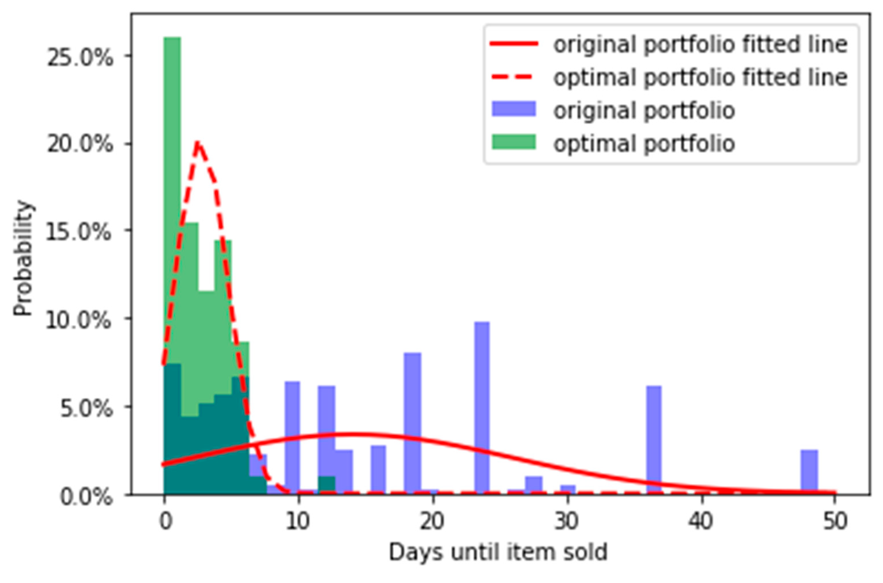
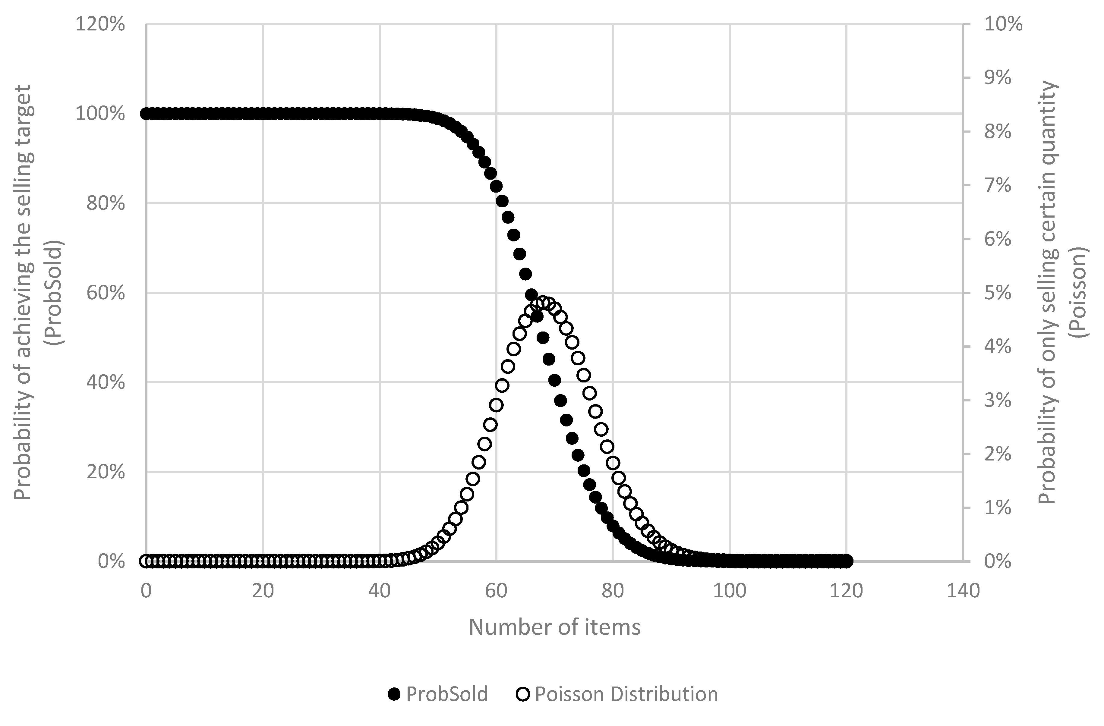
3.2. Determining the Distribution of Listed Items
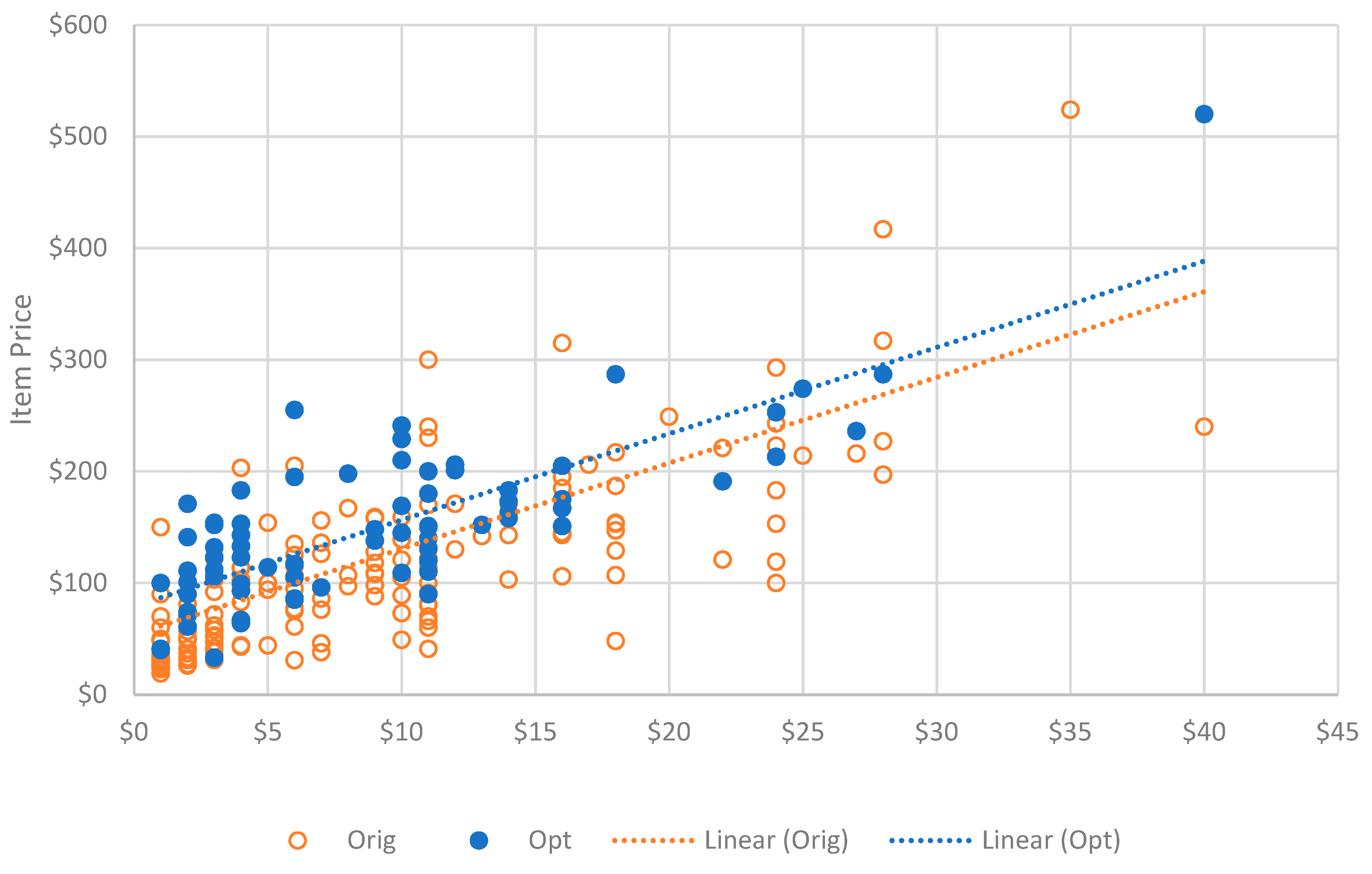
3.3. Duration and Prices
4. Discussion
Author Contributions
Funding
Data Availability Statement
Conflicts of Interest
Appendix A
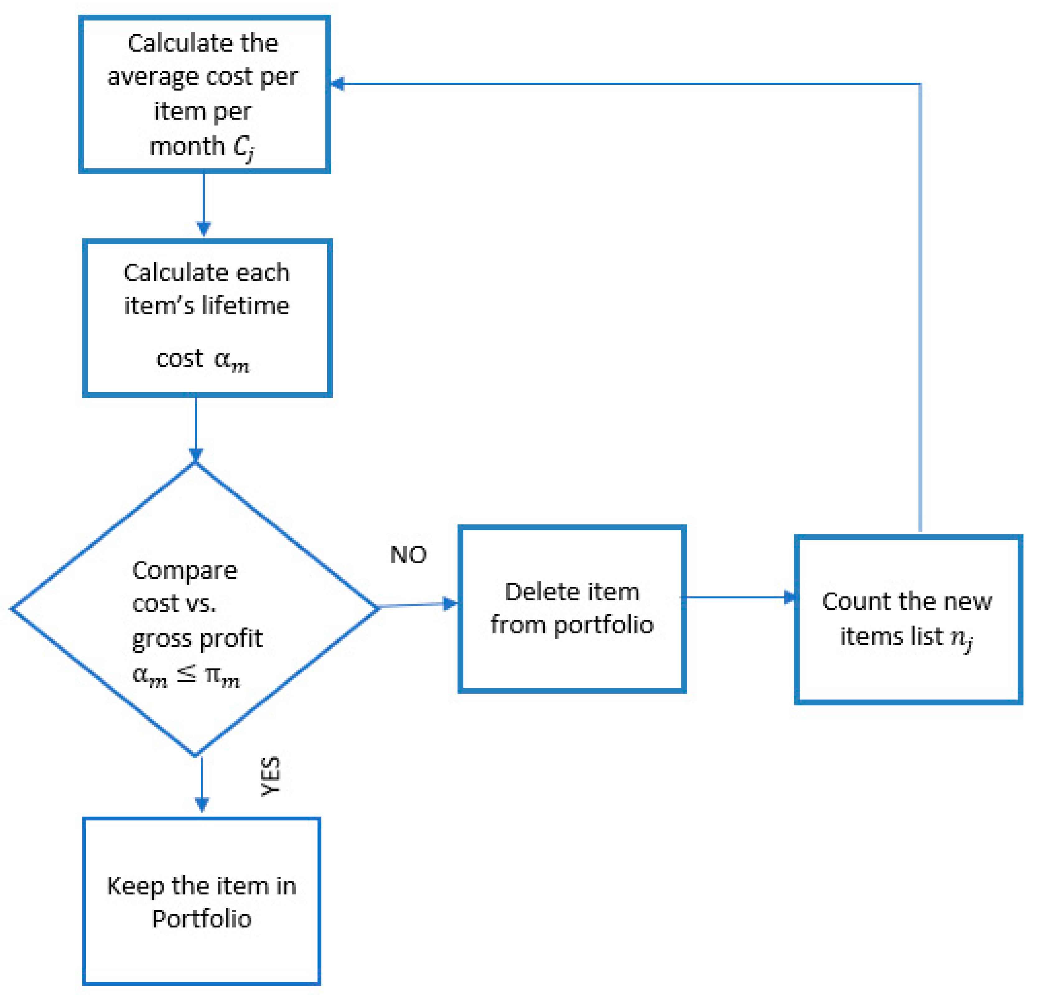
- Let be the number of items kept in the portfolio and let j be the number of iterations (j = 0, 1, 2, …).
- when j = 0, .
- Let C be the total cost of items based on current cycle’s portfolio.
- Let α be the cost of an item, T be the duration of the listing, m be the index of items kept in the jth cycle. The cost to source an item is assumed to increase in proportion to duration based on data from the original portfolio,
- =
- Compare each items’ profit vs. cost such that if >, keep the item in the portfolio. Otherwise, delete the item from the portfolio.
- Recalculate
- Repeat this process until there is no < to obtain the final optimal portfolio.
- proc import out=my_Ebay
- datafile=‘C:\SAS\Ebay’
- dbms=xlsx replace;
- sheet=”Orig data”my_Ebay
- run;
- /*Add column of 1/T=orig d*/
- data my_Ebay;
- set my_Ebay;
- orig_d=1/Dur__Months;
- run;
- sheet="Orig data";
- run;
- proc contents data=my_Ebay;
- run;
- /*Add column of 1/T=orig_d*/
- data my_Ebay;
- set my_Ebay;
- orig_d=1/Dur__Months;
- k=_N_;
- fact_k=fact(k);
- run;
- /*calculate the total orig d*/
- proc sql;
- select sum(orig_d)/count(*) into: final_d
- from my_Ebay;
- quit;
- %put &final_d.;
- /*test count*/
- proc sql;
- select count(*) from my_Ebay;
- quit;
- /*calculate p*/
- data my_Ebay;
- set my_Ebay;
- p=exp(-&final_d.)*(&final_d.*k)/fact_k;
- run;
References
- Acemoglu, Daron. 2007. Equilibrium bias of technology. Econometrica 75: 1371–409. [Google Scholar] [CrossRef] [Green Version]
- Armstrong, Mark. 2006. Competition in two-sided markets. The RAND Journal of Economics 37: 668–91. [Google Scholar] [CrossRef] [Green Version]
- Barney, Jay, and William S. Hesterly. 2014. Strategic Management and Competitive Advantage: Concepts and Cases, 5th ed. Englewood Cliffs: Prentice Hall, pp. 283–301. [Google Scholar]
- Cirman, Andreja, Marko Pahor, and Miroslav Verbic. 2015. Determinants of time on the market in a thin real estate market. Inzinerine Ekonomika-Engineering Economics 26: 4–11. [Google Scholar] [CrossRef] [Green Version]
- Coslor, Erica. 2016. Transparency in an opaque market: Evaluative frictions between “thick” valuation and “thin” price data in the art market. Accounting, Organizations and Society 50: 13–26. [Google Scholar] [CrossRef]
- Deng, Shiming, and Candace A. Yano. 2006. Joint production and pricing decisions with setup costs and capacity constraints. Management Science 52: 741–56. [Google Scholar] [CrossRef]
- Elmaghraby, Wedad, and Pınar Keskinocak. 2003. Dynamic pricing in the presence of inventory considerations: Research overview, current practices, and future directions. Management Science 49: 1287–309. [Google Scholar] [CrossRef]
- Guadix, Jose, Luis Onieva, Jesus Munuzuri, and Pablo Cortés. 2011. An overview of revenue management in service industries: An application to car parks. The Service Industries Journal 31: 91–105. [Google Scholar] [CrossRef]
- Hanson, Robin. 2003. Combinatorial information market design. Information Systems Frontiers 5: 107–19. [Google Scholar] [CrossRef]
- Kendall, Todd D., and Kevin Tsui. 2011. The economics of the long tail. The BE Journal of Economic Analysis & Policy 11: 76. [Google Scholar] [CrossRef]
- Khezr, Peyman. 2015. Time on the market and price change: The case of Sydney housing market. Applied Economics 47: 485–98. [Google Scholar] [CrossRef]
- Knight, John R. 2002. Listing price, time on market, and ultimate selling price: Causes and effects of listing price changes. Real Estate Economics 30: 213–37. [Google Scholar] [CrossRef]
- Lin, Ying. 2020. 10 eBay Statistics You Need to Know in 2020. Oberlo.com. Available online: https://www.oberlo.com/blog/ebay-statistics (accessed on 15 October 2021).
- Severini, Thomas A. 2017. Introduction to Statistical Methods for Financial Models. Boca Raton: Chapman and Hall/CRC. [Google Scholar]
- Sudhir, Karunakaran. 2001. Competitive pricing behavior in the auto market: A structural analysis. Marketing Science 20: 42–60. [Google Scholar] [CrossRef]
- Tesauro, Gerald, and Jeffrey O. Kephart. 2002. Pricing in agent economies using multi-agent Q-learning. Autonomous Agents and Multi-Agent Systems 5: 289–304. [Google Scholar] [CrossRef]
- Yu, Rongshan, Wenxian Yang, and Susanto Rahardja. 2011. Optimal real-time price based on a statistical demand elasticity model of electricity. Paper presented at the 2011 IEEE First International Workshop on Smart Grid Modeling and Simulation (SGMS), Brussels, Belgium, October 17; pp. 90–95. [Google Scholar]


| Listed Quantity | 319 | 600 | 900 | 1200 | 1500 | 1800 | 2100 |
|---|---|---|---|---|---|---|---|
| Lambda (λ) | 68.65 | 129.14 | 193.70 | 258.27 | 322.84 | 387.41 | 451.97 |
| Maximum expected gross profit | USD 5798 | USD 11,633 | USD 18,045 | USD 24,559 | USD 31,142 | USD 37,775 | USD 44,444 |
| Median Split Category | Gross Profit | Item Cost | Weighted Profit (per Item) |
|---|---|---|---|
| High profit, sold fast (HF) | 70.37% | 50.62% | USD 104.85 |
| High profit, sold slow (HS) | 1.23% | 1.23% | USD 22.43 |
| Low profit, sold fast (LF) | 28.40% | 48.15% | USD 5.93 |
| Low profit, sold slow (LS) | 0.00% | 0.00% | USD 0.00 |
Publisher’s Note: MDPI stays neutral with regard to jurisdictional claims in published maps and institutional affiliations. |
© 2022 by the authors. Licensee MDPI, Basel, Switzerland. This article is an open access article distributed under the terms and conditions of the Creative Commons Attribution (CC BY) license (https://creativecommons.org/licenses/by/4.0/).
Share and Cite
Hu, X.; Zak, P.J. A Procedure to Set Prices and Select Inventory in Thinly Traded Markets Using Data from eBay. J. Risk Financial Manag. 2022, 15, 297. https://doi.org/10.3390/jrfm15070297
Hu X, Zak PJ. A Procedure to Set Prices and Select Inventory in Thinly Traded Markets Using Data from eBay. Journal of Risk and Financial Management. 2022; 15(7):297. https://doi.org/10.3390/jrfm15070297
Chicago/Turabian StyleHu, Xinbo, and Paul J. Zak. 2022. "A Procedure to Set Prices and Select Inventory in Thinly Traded Markets Using Data from eBay" Journal of Risk and Financial Management 15, no. 7: 297. https://doi.org/10.3390/jrfm15070297
APA StyleHu, X., & Zak, P. J. (2022). A Procedure to Set Prices and Select Inventory in Thinly Traded Markets Using Data from eBay. Journal of Risk and Financial Management, 15(7), 297. https://doi.org/10.3390/jrfm15070297