
Financial Crises and Business Cycle Implications for Islamic and Non-Islamic Bank Lending in Indonesia

Abstract
:1. Introduction
2. Literature Review
3. Empirical Approach and Definition of Variables
3.1. Background of Financial Crisis and Islamic Banking
3.2. Theoretical Model
4. Empirical Analysis
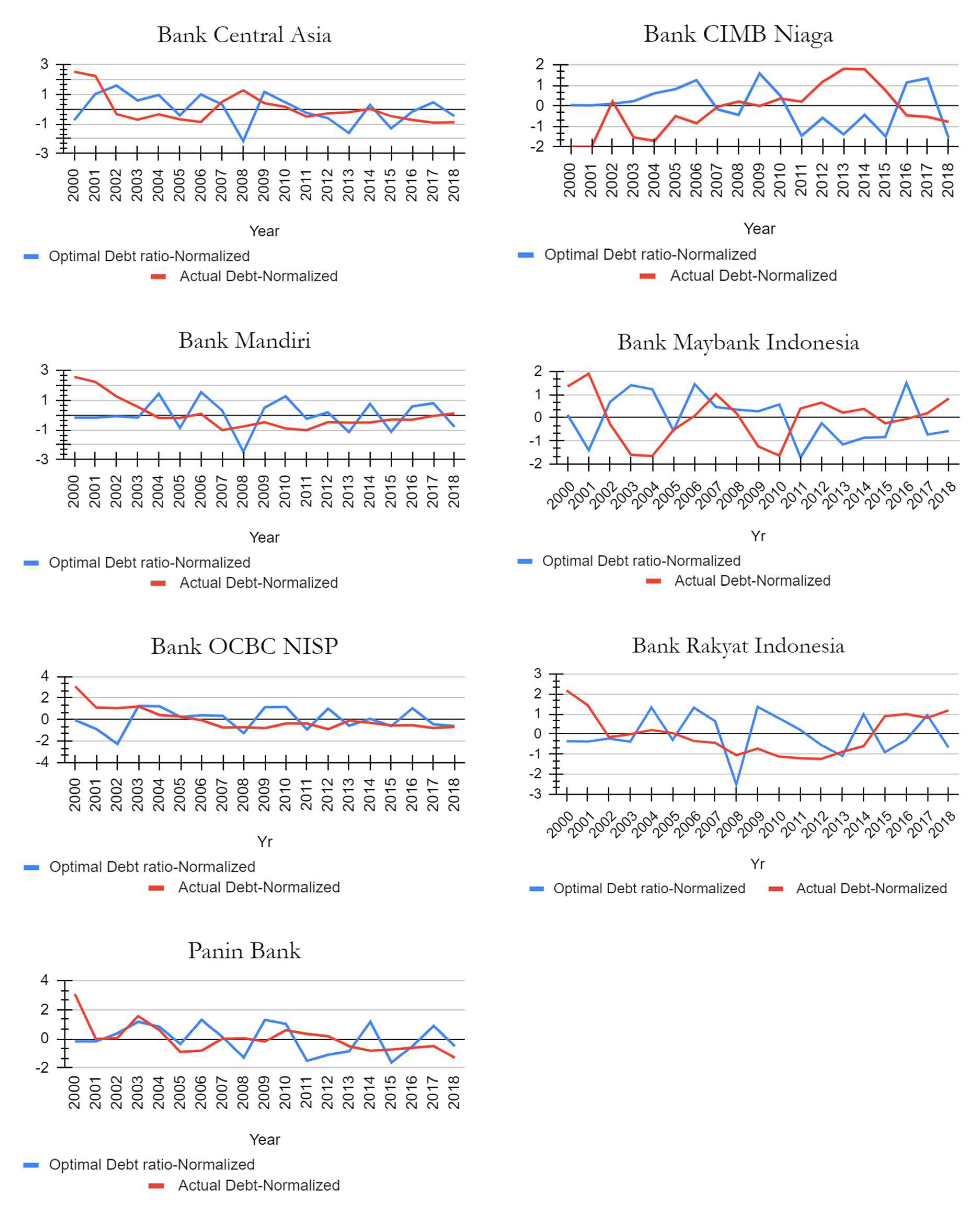
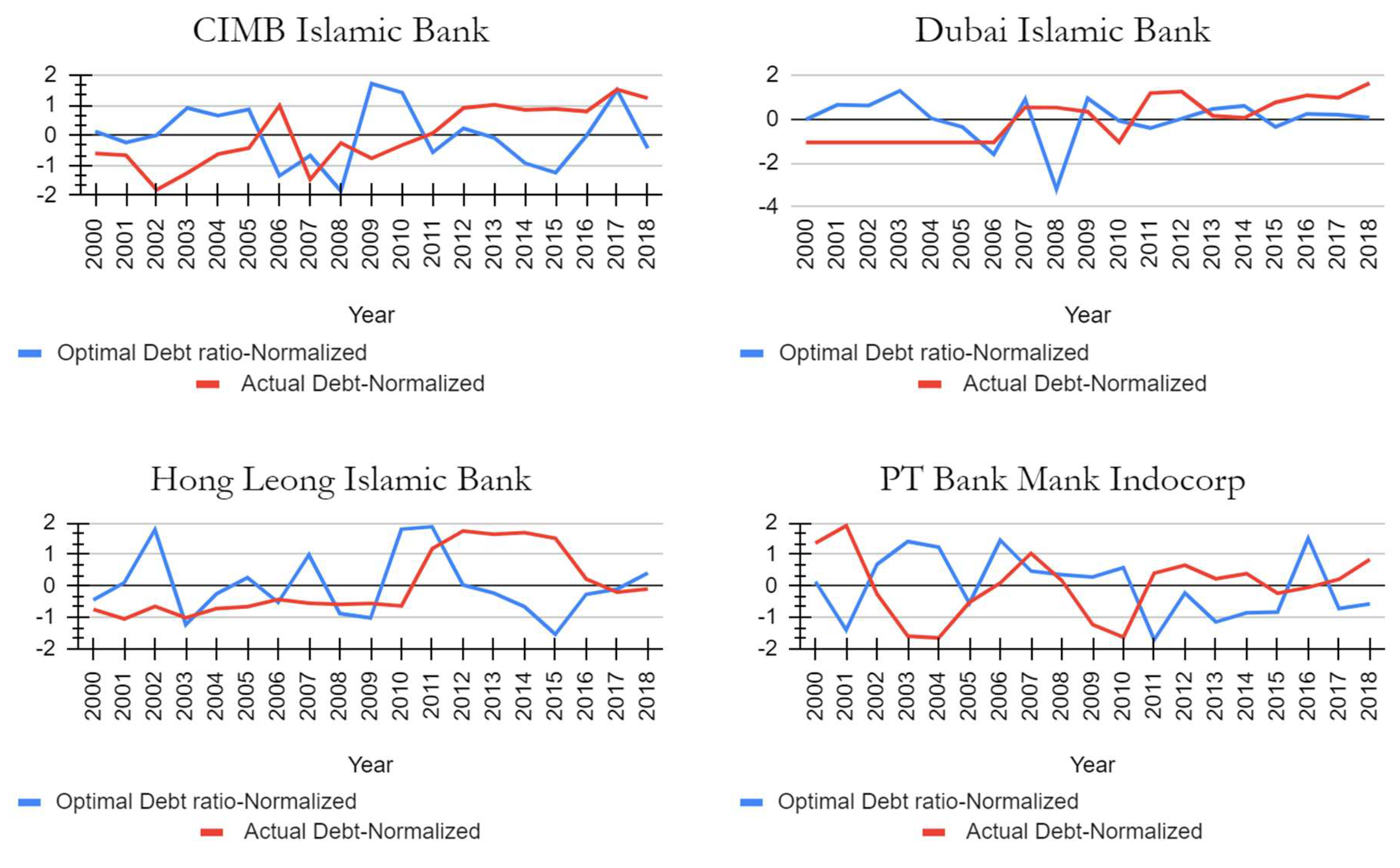
4.1. Graphical Results and Analysis: Actual vs. Optimal Debt
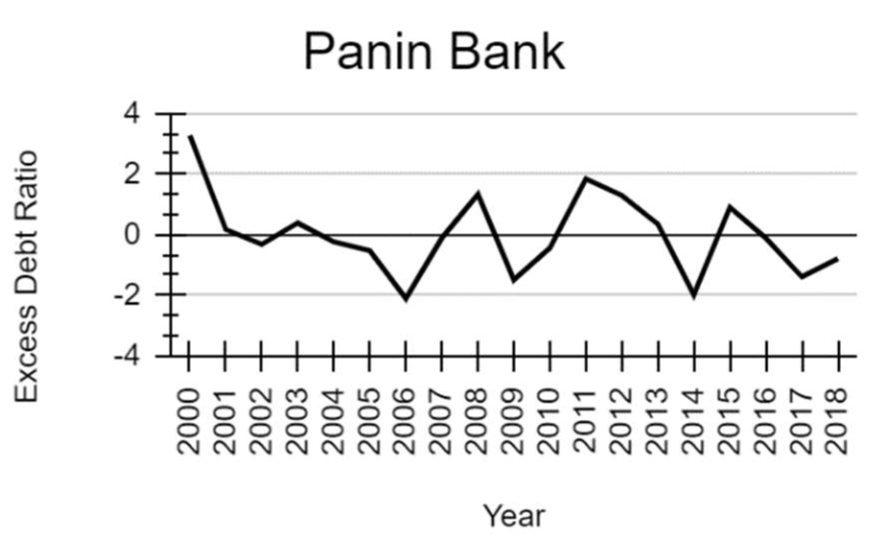
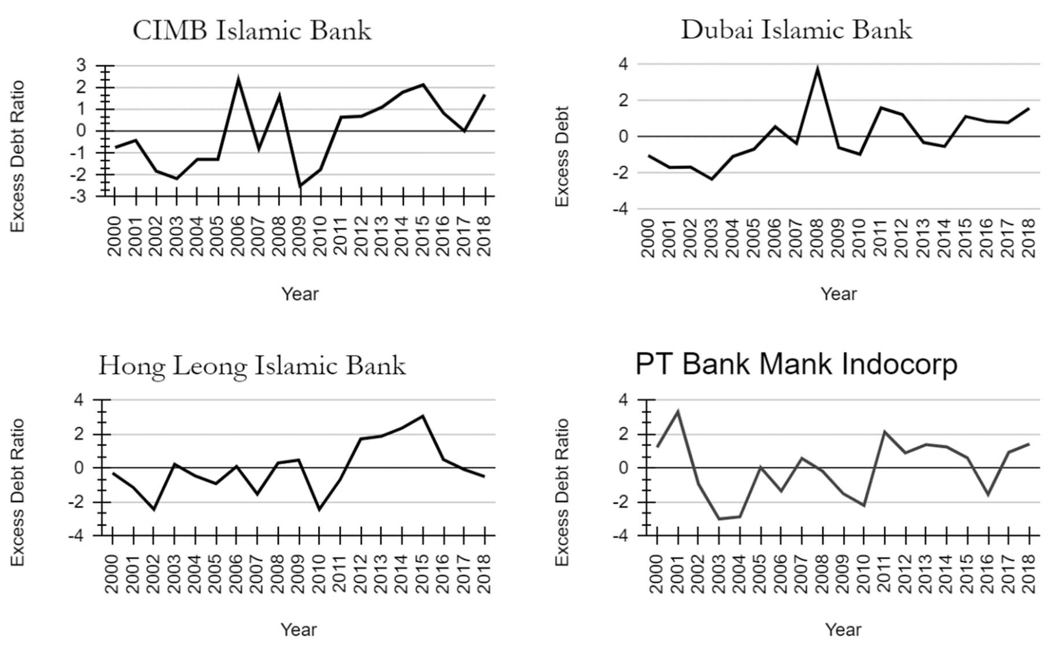
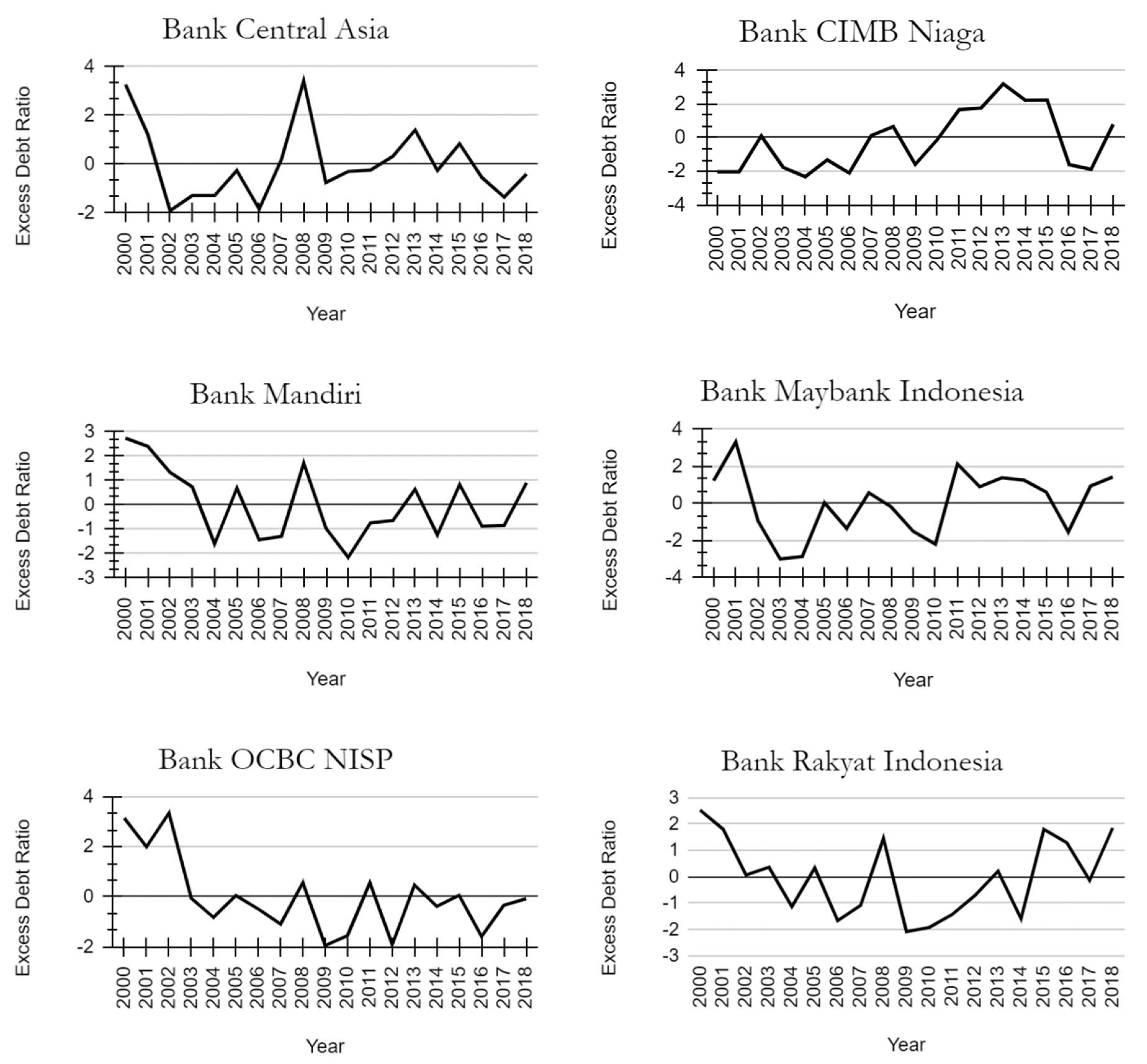
4.2. Graphical Results and Analysis: Excess Debt
5. Conclusions
Funding
Institutional Review Board Statement
Informed Consent Statement
Data Availability Statement
Acknowledgments
Conflicts of Interest
Appendix A
Appendix A.1. Mathematical Derivation of Stein’s Optimal Debt
Appendix A.1.1. Model I
Appendix A.1.2. Model II
Appendix B

| Bank Name | Type | Country |
|---|---|---|
| Central Asia Bank | Conventional Bank | Indonesia |
| CIMB Bank Niaga | Conventional Bank | Indonesia |
| Mandiri Bank | Conventional Bank | Indonesia |
| Maybank Indonesia Bank | Conventional Bank | Indonesia |
| OCBC NISP Bank | Conventional Bank | Indonesia |
| Bank Rakyat Indonesia | Conventional Bank | Indonesia |
| Panin Bank | Conventional Bank | Indonesia |
| CIMB Bank | Islamic Bank | Indonesia |
| Dubai Islamic Bank | Islamic Bank | Indonesia |
| Hong Leong Bank | Islamic Bank | Indonesia |
| PT Mank Indocorp Bank | Islamic Bank | Indonesia |
Appendix C
| Bank | Year | Capital Gains/(Losses), (r) | Interest Rate (i) | Beta (Productivity of Capital, β) | Beta Variance (αy(t)) | Half Square of Capital Gain Variance | Correlation of Interest and Capital Gain Variables | Interest Rate Variance | Capital Gain Variance | Correlation and Variances of Interest and Capital Gain | Std. Deviation of Interest Rate | Std. Deviation of Capital Gain | 2 × (Correlation and Variances of Interest and Capital Gain) | Risk | Optimal Debt Ratio, ƒ*(t) | Normalized Optimal Debt Ratio | Actual Debt Ratio | Normalized Actual Debt Ratio | Excess Debt |
|---|---|---|---|---|---|---|---|---|---|---|---|---|---|---|---|---|---|---|---|
| CIMB Islamic Bank | 2000 | 0.0096 | 0.0258 | 0.3368 | (0.020) | 0.000 | (0.36) | (0.0098) | 0.3260 | 0.0011 | 0.0133 | 0.6503 | 0.0023 | 0.661 | 0.52 | 0.13 | 0.0494 | (0.61) | (0.74) |
| 2001 | −0.0965 | 0.0243 | 0.3065 | (0.051) | 0.005 | (0.36) | (0.0113) | 0.0636 | 0.0003 | 0.0133 | 0.6503 | 0.0005 | 0.663 | 0.35 | (0.25) | 0.0485 | (0.67) | (0.42) | |
| 2002 | −0.0424 | 0.0209 | 0.2710 | (0.086) | 0.001 | (0.36) | (0.0147) | 1.2205 | 0.0064 | 0.0133 | 0.6503 | 0.0127 | 0.651 | 0.46 | (0.00) | 0.0296 | (1.82) | (1.82) | |
| 2003 | 0.2783 | 0.0188 | 0.3168 | (0.040) | 0.039 | (0.36) | (0.0168) | −0.1798 | (0.0011) | 0.0133 | 0.6503 | (0.0021) | 0.666 | 0.87 | 0.91 | 0.0388 | (1.26) | (2.16) | |
| 2004 | 0.1899 | 0.0286 | 0.3015 | (0.056) | 0.018 | (0.36) | (0.0070) | −0.0292 | (0.0001) | 0.0133 | 0.6503 | (0.0001) | 0.664 | 0.75 | 0.66 | 0.0491 | (0.63) | (1.28) | |
| 2005 | 0.2486 | 0.0191 | 0.3377 | (0.020) | 0.031 | (0.36) | (0.0165) | 0.2895 | 0.0017 | 0.0133 | 0.6503 | 0.0034 | 0.660 | 0.84 | 0.86 | 0.0524 | (0.43) | (1.28) | |
| 2006 | 2.3655 | 0.0197 | 0.3522 | (0.005) | 2.798 | (0.36) | (0.0159) | −0.2307 | (0.0013) | 0.0133 | 0.6503 | (0.0026) | 0.666 | (0.14) | (1.35) | 0.0755 | 0.99 | 2.33 | |
| 2007 | −0.1993 | 0.0339 | 0.4041 | 0.047 | 0.020 | (0.36) | (0.0017) | −0.6142 | (0.0004) | 0.0133 | 0.6503 | (0.0007) | 0.664 | 0.16 | (0.68) | 0.0352 | (1.47) | (0.80) | |
| 2008 | −0.4600 | 0.0373 | 0.4205 | 0.063 | 0.106 | (0.36) | 0.0017 | 0.8440 | (0.0005) | 0.0133 | 0.6503 | (0.0010) | 0.665 | (0.37) | (1.85) | 0.0551 | (0.26) | 1.59 | |
| 2009 | 1.1797 | 0.0252 | 0.4292 | 0.072 | 0.696 | (0.36) | (0.0104) | 0.0327 | 0.0001 | 0.0133 | 0.6503 | 0.0002 | 0.663 | 1.23 | 1.72 | 0.0468 | (0.77) | (2.49) | |
| 2010 | 0.5658 | 0.0374 | 0.4022 | 0.045 | 0.160 | (0.36) | 0.0018 | −0.5646 | 0.0004 | 0.0133 | 0.6503 | 0.0007 | 0.663 | 1.10 | 1.42 | 0.0540 | (0.33) | (1.74) | |
| 2011 | −0.1541 | 0.0476 | 0.4411 | 0.084 | 0.012 | (0.36) | 0.0120 | 1.1362 | (0.0049) | 0.0133 | 0.6503 | (0.0097) | 0.673 | 0.21 | (0.57) | 0.0605 | 0.07 | 0.64 | |
| 2012 | 0.0637 | 0.0442 | 0.3922 | 0.035 | 0.002 | (0.36) | 0.0086 | 0.3179 | (0.0010) | 0.0133 | 0.6503 | (0.0020) | 0.665 | 0.56 | 0.23 | 0.0743 | 0.91 | 0.68 | |
| 2013 | −0.0338 | 0.0422 | 0.3907 | 0.033 | 0.001 | (0.36) | 0.0066 | 0.1408 | (0.0003) | 0.0133 | 0.6503 | (0.0007) | 0.664 | 0.42 | (0.09) | 0.0760 | 1.01 | 1.10 | |
| 2014 | −0.2548 | 0.0415 | 0.3313 | (0.026) | 0.032 | (0.36) | 0.0059 | −0.0714 | 0.0002 | 0.0133 | 0.6503 | 0.0003 | 0.663 | 0.04 | (0.93) | 0.0732 | 0.84 | 1.77 | |
| 2015 | −0.3276 | 0.0405 | 0.3714 | 0.014 | 0.054 | (0.36) | 0.0049 | 0.2717 | (0.0005) | 0.0133 | 0.6503 | (0.0010) | 0.664 | (0.10) | (1.25) | 0.0737 | 0.87 | 2.12 | |
| 2016 | −0.0089 | 0.0504 | 0.3416 | (0.016) | 0.000 | (0.36) | 0.0148 | −0.1599 | 0.0008 | 0.0133 | 0.6503 | 0.0017 | 0.662 | 0.45 | (0.02) | 0.0724 | 0.79 | 0.81 | |
| 2017 | 0.6666 | 0.0516 | 0.3112 | (0.046) | 0.222 | (0.36) | 0.0160 | −0.1599 | 0.0009 | 0.0133 | 0.6503 | 0.0018 | 0.662 | 1.13 | 1.51 | 0.0843 | 1.52 | 0.01 | |
| 2018 | −0.1107 | 0.0666 | 0.3293 | (0.028) | 0.006 | (0.36) | 0.0310 | −0.1599 | 0.0018 | 0.0133 | 0.6503 | 0.0035 | 0.660 | 0.27 | (0.43) | 0.0796 | 1.24 | 1.67 |
| Bank | Year | Capital Gains/(Losses), (r) | Interest Rate (i) | Beta (Productivity of Capital, β) | Beta Variance (αy(t)) | Half Square of Capital Gain Variance | Correlation of Interest and Capital Gain Variables | Interest Rate Variance | Capital Gain Variance | Correlation and Variances of Interest and Capital Gain | Std. Deviation of Interest Rate | Std. Deviation of Capital Gain | 2 × (Correlation and Variances of Interest and Capital Gain) | Risk | Optimal Debt Ratio, ƒ*(t) | Normalized Optimal Debt Ratio | Actual Debt Ratio | Normalized Actual Debt Ratio | Excess Debt |
|---|---|---|---|---|---|---|---|---|---|---|---|---|---|---|---|---|---|---|---|
| Dubai Islamic Bank | 2000 | 0.0000 | 0.0258 | 0.6658 | 0.278 | 0.000 | (0.27) | (0.0098) | 0.3260 | 0.0009 | 0.0133 | 0.7859 | 0.0017 | 0.797 | 0.46 | (0.02) | 0.0000 | (1.06) | (1.04) |
| 2001 | 0.2875 | 0.0243 | 0.6203 | 0.232 | 0.041 | (0.27) | (0.0113) | 0.0636 | 0.0002 | 0.0133 | 0.7859 | 0.0004 | 0.799 | 0.76 | 0.65 | 0.0000 | (1.06) | (1.71) | |
| 2002 | 0.2524 | 0.0209 | 0.5176 | 0.130 | 0.032 | (0.27) | (0.0147) | 1.2205 | 0.0048 | 0.0133 | 0.7859 | 0.0097 | 0.790 | 0.75 | 0.62 | 0.0000 | (1.06) | (1.68) | |
| 2003 | 0.8120 | 0.0188 | 0.5501 | 0.162 | 0.330 | (0.27) | (0.0168) | −0.1798 | (0.0008) | 0.0133 | 0.7859 | (0.0016) | 0.801 | 1.06 | 1.29 | 0.0000 | (1.06) | (2.35) | |
| 2004 | 1.9775 | 0.0286 | 0.3991 | 0.011 | 1.955 | (0.27) | (0.0070) | −0.0292 | (0.0001) | 0.0133 | 0.7859 | (0.0001) | 0.799 | 0.48 | 0.03 | 0.0000 | (1.06) | (1.09) | |
| 2005 | 2.1303 | 0.0191 | 0.4578 | 0.070 | 2.269 | (0.27) | (0.0165) | 0.2895 | 0.0013 | 0.0133 | 0.7859 | 0.0026 | 0.797 | 0.29 | (0.37) | 0.0000 | (1.06) | (0.69) | |
| 2006 | −0.4808 | 0.0197 | 0.3583 | (0.030) | 0.116 | (0.27) | (0.0159) | −0.2307 | (0.0010) | 0.0133 | 0.7859 | (0.0020) | 0.801 | (0.29) | (1.61) | 0.0000 | (1.06) | 0.55 | |
| 2007 | 0.4568 | 0.0339 | 0.5096 | 0.122 | 0.104 | (0.27) | (0.0017) | −0.6142 | (0.0003) | 0.0133 | 0.7859 | (0.0006) | 0.800 | 0.88 | 0.90 | 0.0327 | 0.53 | (0.37) | |
| 2008 | −0.8265 | 0.0373 | 0.4183 | 0.030 | 0.342 | (0.27) | 0.0017 | 0.8440 | (0.0004) | 0.0133 | 0.7859 | (0.0008) | 0.800 | (1.02) | (3.19) | 0.0325 | 0.52 | 3.71 | |
| 2009 | 0.4674 | 0.0252 | 0.4615 | 0.073 | 0.109 | (0.27) | (0.0104) | 0.0327 | 0.0001 | 0.0133 | 0.7859 | 0.0002 | 0.799 | 0.90 | 0.94 | 0.0286 | 0.34 | (0.61) | |
| 2010 | −0.0137 | 0.0374 | 0.2758 | (0.112) | 0.000 | (0.27) | 0.0018 | −0.5646 | 0.0003 | 0.0133 | 0.7859 | 0.0006 | 0.799 | 0.42 | (0.09) | 0.0000 | (1.06) | (0.97) | |
| 2011 | −0.1101 | 0.0476 | 0.3097 | (0.078) | 0.006 | (0.27) | 0.0120 | 1.1362 | (0.0037) | 0.0133 | 0.7859 | (0.0074) | 0.807 | 0.27 | (0.41) | 0.0461 | 1.18 | 1.59 | |
| 2012 | 0.0361 | 0.0442 | 0.2719 | (0.116) | 0.001 | (0.27) | 0.0086 | 0.3179 | (0.0007) | 0.0133 | 0.7859 | (0.0015) | 0.801 | 0.47 | 0.02 | 0.0474 | 1.25 | 1.23 | |
| 2013 | 1.7768 | 0.0422 | 0.2734 | (0.115) | 1.578 | (0.27) | 0.0066 | 0.1408 | (0.0003) | 0.0133 | 0.7859 | (0.0005) | 0.800 | 0.68 | 0.47 | 0.0248 | 0.15 | (0.32) | |
| 2014 | 0.2873 | 0.0415 | 0.2954 | (0.093) | 0.041 | (0.27) | 0.0059 | −0.0714 | 0.0001 | 0.0133 | 0.7859 | 0.0002 | 0.799 | 0.74 | 0.60 | 0.0230 | 0.06 | (0.54) | |
| 2015 | −0.1043 | 0.0405 | 0.2601 | (0.128) | 0.005 | (0.27) | 0.0049 | 0.2717 | (0.0004) | 0.0133 | 0.7859 | (0.0007) | 0.800 | 0.30 | (0.36) | 0.0374 | 0.76 | 1.12 | |
| 2016 | 0.1265 | 0.0504 | 0.2329 | (0.155) | 0.008 | (0.27) | 0.0148 | −0.1599 | 0.0006 | 0.0133 | 0.7859 | 0.0013 | 0.798 | 0.57 | 0.24 | 0.0440 | 1.08 | 0.85 | |
| 2017 | 0.1113 | 0.0516 | 0.2479 | (0.140) | 0.006 | (0.27) | 0.0160 | −0.1599 | 0.0007 | 0.0133 | 0.7859 | 0.0014 | 0.798 | 0.55 | 0.20 | 0.0418 | 0.97 | 0.78 | |
| 2018 | 0.0749 | 0.0666 | 0.2471 | (0.141) | 0.003 | (0.27) | 0.0310 | −0.1599 | 0.0013 | 0.0133 | 0.7859 | 0.0027 | 0.797 | 0.50 | 0.07 | 0.0553 | 1.63 | 1.56 |
| Bank | Year | Capital Gains/(Losses), (r) | Interest Rate (i) | Beta (Productivity of Capital, β) | Beta Variance (αy(t)) | Half Square of Capital Gain Variance | Correlation of Interest and Capital Gain Variables | Interest Rate Variance | Capital Gain Variance | Correlation and Variances of Interest and Capital Gain | Std. Deviation of Interest Rate | Std. Deviation of Capital Gain | 2 × (Correlation and Variances of Interest and Capital Gain) | Risk | Optimal Debt Ratio, ƒ*(t) | Normalized Optimal Debt Ratio | Actual Debt Ratio | Normalized Actual Debt Ratio | Excess Debt |
|---|---|---|---|---|---|---|---|---|---|---|---|---|---|---|---|---|---|---|---|
| Hong Leong Islamic Bank | 2000 | 0.0096 | 0.0258 | 0.5835 | 0.216 | 0.000 | 0.15 | (0.0098) | 0.3260 | (0.0005) | 0.0133 | 0.2561 | (0.0010) | 0.270 | 1.30 | (0.45) | 0.0057 | (0.75) | (0.30) |
| 2001 | 0.1144 | 0.0243 | 0.4867 | 0.119 | 0.007 | 0.15 | (0.0113) | 0.0636 | (0.0001) | 0.0133 | 0.2561 | (0.0002) | 0.270 | 1.67 | 0.09 | 0.0000 | (1.05) | (1.15) | |
| 2002 | 0.6370 | 0.0209 | 0.4504 | 0.083 | 0.203 | 0.15 | (0.0147) | 1.2205 | (0.0027) | 0.0133 | 0.2561 | (0.0054) | 0.275 | 2.83 | 1.78 | 0.0075 | (0.65) | (2.43) | |
| 2003 | −0.1364 | 0.0188 | 0.4679 | 0.100 | 0.009 | 0.15 | (0.0168) | −0.1798 | 0.0005 | 0.0133 | 0.2561 | 0.0009 | 0.268 | 0.76 | (1.24) | 0.0007 | (1.02) | 0.22 | |
| 2004 | 0.0476 | 0.0286 | 0.3300 | (0.038) | 0.001 | 0.15 | (0.0070) | −0.0292 | 0.0000 | 0.0133 | 0.2561 | 0.0001 | 0.269 | 1.43 | (0.26) | 0.0062 | (0.73) | (0.47) | |
| 2005 | 0.1459 | 0.0191 | 0.2556 | (0.112) | 0.011 | 0.15 | (0.0165) | 0.2895 | (0.0007) | 0.0133 | 0.2561 | (0.0014) | 0.271 | 1.78 | 0.26 | 0.0072 | (0.67) | (0.92) | |
| 2006 | −0.0139 | 0.0197 | 0.3151 | (0.052) | 0.000 | 0.15 | (0.0159) | −0.2307 | 0.0006 | 0.0133 | 0.2561 | 0.0011 | 0.268 | 1.25 | (0.53) | 0.0116 | (0.43) | 0.09 | |
| 2007 | 0.3373 | 0.0339 | 0.4206 | 0.053 | 0.057 | 0.15 | (0.0017) | −0.6142 | 0.0002 | 0.0133 | 0.2561 | 0.0003 | 0.269 | 2.28 | 0.98 | 0.0094 | (0.55) | (1.54) | |
| 2008 | −0.0595 | 0.0373 | 0.4176 | 0.050 | 0.002 | 0.15 | 0.0017 | 0.8440 | 0.0002 | 0.0133 | 0.2561 | 0.0004 | 0.269 | 1.00 | (0.88) | 0.0087 | (0.59) | 0.29 | |
| 2009 | −0.0942 | 0.0252 | 0.5064 | 0.139 | 0.004 | 0.15 | (0.0104) | 0.0327 | (0.0001) | 0.0133 | 0.2561 | (0.0001) | 0.270 | 0.90 | (1.03) | 0.0092 | (0.56) | 0.46 | |
| 2010 | 0.6427 | 0.0374 | 0.3539 | (0.014) | 0.207 | 0.15 | 0.0018 | −0.5646 | (0.0002) | 0.0133 | 0.2561 | (0.0003) | 0.270 | 2.84 | 1.80 | 0.0077 | (0.64) | (2.44) | |
| 2011 | 0.6704 | 0.0476 | 0.2554 | (0.112) | 0.225 | 0.15 | 0.0120 | 1.1362 | 0.0021 | 0.0133 | 0.2561 | 0.0042 | 0.265 | 2.89 | 1.87 | 0.0418 | 1.18 | (0.70) | |
| 2012 | 0.1200 | 0.0442 | 0.3313 | (0.036) | 0.007 | 0.15 | 0.0086 | 0.3179 | 0.0004 | 0.0133 | 0.2561 | 0.0008 | 0.269 | 1.63 | 0.03 | 0.0523 | 1.74 | 1.71 | |
| 2013 | 0.0662 | 0.0422 | 0.3155 | (0.052) | 0.002 | 0.15 | 0.0066 | 0.1408 | 0.0001 | 0.0133 | 0.2561 | 0.0003 | 0.269 | 1.45 | (0.23) | 0.0504 | 1.64 | 1.87 | |
| 2014 | −0.0156 | 0.0415 | 0.3095 | (0.058) | 0.000 | 0.15 | 0.0059 | −0.0714 | (0.0001) | 0.0133 | 0.2561 | (0.0001) | 0.270 | 1.15 | (0.67) | 0.0514 | 1.69 | 2.35 | |
| 2015 | −0.1664 | 0.0405 | 0.3262 | (0.041) | 0.014 | 0.15 | 0.0049 | 0.2717 | 0.0002 | 0.0133 | 0.2561 | 0.0004 | 0.269 | 0.55 | (1.55) | 0.0481 | 1.51 | 3.06 | |
| 2016 | 0.0688 | 0.0504 | 0.2860 | (0.082) | 0.002 | 0.15 | 0.0148 | −0.1599 | (0.0004) | 0.0133 | 0.2561 | (0.0007) | 0.270 | 1.42 | (0.28) | 0.0238 | 0.22 | 0.49 | |
| 2017 | 0.1036 | 0.0516 | 0.2923 | (0.075) | 0.005 | 0.15 | 0.0160 | −0.1599 | (0.0004) | 0.0133 | 0.2561 | (0.0008) | 0.270 | 1.53 | (0.11) | 0.0160 | (0.20) | (0.09) | |
| 2018 | 0.2391 | 0.0666 | 0.2804 | (0.087) | 0.029 | 0.15 | 0.0310 | −0.1599 | (0.0008) | 0.0133 | 0.2561 | (0.0015) | 0.271 | 1.89 | 0.40 | 0.0178 | (0.10) | (0.51) |
| Bank | Year | Capital Gains/(Losses), (r) | Interest Rate (i) | Beta (Productivity of Capital, β) | Beta Variance (αy(t)) | Half Square of Capital Gain Variance | Correlation of Interest and Capital Gain Variables | Interest Rate Variance | Capital Gain Variance | Correlation and Variances of Interest and Capital Gain | Std. Deviation of Interest Rate | Std. Deviation of Capital Gain | 2 × (Correlation and Variances of Interest and Capital Gain) | Risk | Optimal Debt Ratio, ƒ*(t) | Normalized Optimal Debt Ratio | Actual Debt Ratio | Normalized Actual Debt Ratio | Excess Debt |
|---|---|---|---|---|---|---|---|---|---|---|---|---|---|---|---|---|---|---|---|
| PT Bank Mank Indocorp | 2000 | 0.0096 | 0.0258 | 1.0100 | (0.003) | 0.000 | (0.23) | (0.0098) | 0.3260 | 0.0007 | 0.0133 | 0.6297 | 0.0015 | 0.641 | 1.55 | 0.13 | 0.1110 | 1.35 | 1.22 |
| 2001 | −0.4186 | 0.0243 | 5.3172 | 4.304 | 0.088 | (0.23) | (0.0113) | 0.0636 | 0.0002 | 0.0133 | 0.6297 | 0.0003 | 0.643 | 0.75 | (1.40) | 0.1292 | 1.91 | 3.31 | |
| 2002 | 0.1956 | 0.0209 | 0.8513 | (0.162) | 0.019 | (0.23) | (0.0147) | 1.2205 | 0.0041 | 0.0133 | 0.6297 | 0.0083 | 0.635 | 1.85 | 0.68 | 0.0581 | (0.27) | (0.95) | |
| 2003 | 1.3398 | 0.0188 | 0.9427 | (0.070) | 0.898 | (0.23) | (0.0168) | −0.1798 | (0.0007) | 0.0133 | 0.6297 | (0.0014) | 0.644 | 2.23 | 1.41 | 0.0144 | (1.60) | (3.01) | |
| 2004 | 0.5260 | 0.0286 | 0.9078 | (0.105) | 0.138 | (0.23) | (0.0070) | −0.0292 | (0.0000) | 0.0133 | 0.6297 | (0.0001) | 0.643 | 2.13 | 1.23 | 0.0126 | (1.66) | (2.89) | |
| 2005 | −0.2082 | 0.0191 | 0.7268 | (0.286) | 0.022 | (0.23) | (0.0165) | 0.2895 | 0.0011 | 0.0133 | 0.6297 | 0.0022 | 0.641 | 1.19 | (0.56) | 0.0495 | (0.53) | 0.03 | |
| 2006 | 0.7075 | 0.0197 | 0.7680 | (0.245) | 0.250 | (0.23) | (0.0159) | −0.2307 | (0.0008) | 0.0133 | 0.6297 | (0.0017) | 0.645 | 2.25 | 1.45 | 0.0696 | 0.09 | (1.36) | |
| 2007 | 0.1469 | 0.0339 | 0.6602 | (0.353) | 0.011 | (0.23) | (0.0017) | −0.6142 | (0.0002) | 0.0133 | 0.6297 | (0.0005) | 0.643 | 1.73 | 0.47 | 0.1006 | 1.03 | 0.56 | |
| 2008 | 0.1070 | 0.0373 | 1.0879 | 0.075 | 0.006 | (0.23) | 0.0017 | 0.8440 | (0.0003) | 0.0133 | 0.6297 | (0.0007) | 0.644 | 1.67 | 0.35 | 0.0721 | 0.16 | (0.19) | |
| 2009 | 0.0655 | 0.0252 | 0.8851 | (0.128) | 0.002 | (0.23) | (0.0104) | 0.0327 | 0.0001 | 0.0133 | 0.6297 | 0.0002 | 0.643 | 1.64 | 0.28 | 0.0264 | (1.24) | (1.52) | |
| 2010 | 1.8075 | 0.0374 | 0.9296 | (0.083) | 1.633 | (0.23) | 0.0018 | −0.5646 | 0.0002 | 0.0133 | 0.6297 | 0.0005 | 0.642 | 1.79 | 0.57 | 0.0133 | (1.64) | (2.21) | |
| 2011 | −0.4712 | 0.0476 | 0.7533 | (0.260) | 0.111 | (0.23) | 0.0120 | 1.1362 | (0.0032) | 0.0133 | 0.6297 | (0.0063) | 0.649 | 0.59 | (1.72) | 0.0799 | 0.40 | 2.12 | |
| 2012 | −0.0850 | 0.0442 | 0.7047 | (0.308) | 0.004 | (0.23) | 0.0086 | 0.3179 | (0.0006) | 0.0133 | 0.6297 | (0.0013) | 0.644 | 1.37 | (0.23) | 0.0882 | 0.65 | 0.89 | |
| 2013 | −0.3435 | 0.0422 | 0.8080 | (0.205) | 0.059 | (0.23) | 0.0066 | 0.1408 | (0.0002) | 0.0133 | 0.6297 | (0.0004) | 0.643 | 0.88 | (1.15) | 0.0741 | 0.22 | 1.37 | |
| 2014 | −0.2701 | 0.0415 | 0.6546 | (0.358) | 0.036 | (0.23) | 0.0059 | −0.0714 | 0.0001 | 0.0133 | 0.6297 | 0.0002 | 0.643 | 1.03 | (0.86) | 0.0794 | 0.38 | 1.25 | |
| 2015 | −0.2625 | 0.0405 | 0.6685 | (0.344) | 0.034 | (0.23) | 0.0049 | 0.2717 | (0.0003) | 0.0133 | 0.6297 | (0.0006) | 0.644 | 1.05 | (0.84) | 0.0590 | (0.24) | 0.60 | |
| 2016 | 1.0347 | 0.0504 | 0.5866 | (0.426) | 0.535 | (0.23) | 0.0148 | −0.1599 | 0.0005 | 0.0133 | 0.6297 | 0.0011 | 0.642 | 2.28 | 1.50 | 0.0651 | (0.05) | (1.56) | |
| 2017 | −0.2263 | 0.0516 | 0.5460 | (0.467) | 0.026 | (0.23) | 0.0160 | −0.1599 | 0.0006 | 0.0133 | 0.6297 | 0.0012 | 0.642 | 1.11 | (0.73) | 0.0735 | 0.20 | 0.93 | |
| 2018 | −0.1732 | 0.0666 | 0.4354 | (0.577) | 0.015 | (0.23) | 0.0310 | −0.1599 | 0.0011 | 0.0133 | 0.6297 | 0.0023 | 0.641 | 1.19 | (0.58) | 0.0941 | 0.83 | 1.41 |
| Bank | Year | Capital Gains/(Losses), (r) | Interest Rate (i) | Beta (Productivity of Capital, β) | Beta Variance (αy(t)) | Half Square of Capital Gain Variance | Correlation of Interest and Capital Gain Variables | Interest Rate Variance | Capital Gain Variance | Correlation and Variances of Interest and Capital Gain | Std. Deviation of Interest Rate | Std. Deviation of Capital Gain | 2 × (Correlation and Variances of Interest and Capital Gain) | Risk | Optimal debt Ratio, ƒ*(t) | Normalized Optimal Debt Ratio | Actual Debt Ratio | Normalized Actual Debt Ratio | Excess Debt |
|---|---|---|---|---|---|---|---|---|---|---|---|---|---|---|---|---|---|---|---|
| Bank Central Asia | 2000 | 0.0096 | 0.0258 | 1.6925 | 0.812 | 0.000 | (0.46) | (0.0098) | 0.3260 | 0.0015 | 0.0133 | 0.3366 | 0.0029 | 0.347 | 2.50 | (0.75) | 0.0157 | 2.50 | 3.26 |
| 2001 | 0.6546 | 0.0243 | 1.3646 | 0.484 | 0.214 | (0.46) | (0.0113) | 0.0636 | 0.0003 | 0.0133 | 0.3366 | 0.0007 | 0.349 | 3.71 | 1.02 | 0.0144 | 2.23 | 1.21 | |
| 2002 | 0.9932 | 0.0209 | 1.2234 | 0.343 | 0.493 | (0.46) | (0.0147) | 1.2205 | 0.0082 | 0.0133 | 0.3366 | 0.0165 | 0.333 | 4.10 | 1.58 | 0.0033 | (0.34) | (1.92) | |
| 2003 | 0.4399 | 0.0188 | 1.0072 | 0.126 | 0.097 | (0.46) | (0.0168) | −0.1798 | (0.0014) | 0.0133 | 0.3366 | (0.0028) | 0.353 | 3.41 | 0.58 | 0.0016 | (0.72) | (1.30) | |
| 2004 | 0.6291 | 0.0286 | 0.9449 | 0.064 | 0.198 | (0.46) | (0.0070) | −0.0292 | (0.0001) | 0.0133 | 0.3366 | (0.0002) | 0.350 | 3.67 | 0.95 | 0.0032 | (0.35) | (1.30) | |
| 2005 | 0.0796 | 0.0191 | 0.9418 | 0.061 | 0.003 | (0.46) | (0.0165) | 0.2895 | 0.0022 | 0.0133 | 0.3366 | 0.0044 | 0.346 | 2.72 | (0.43) | 0.0018 | (0.69) | (0.27) | |
| 2006 | 0.6682 | 0.0197 | 0.9890 | 0.108 | 0.223 | (0.46) | (0.0159) | −0.2307 | (0.0017) | 0.0133 | 0.3366 | (0.0034) | 0.353 | 3.69 | 0.99 | 0.0010 | (0.87) | (1.85) | |
| 2007 | 0.3442 | 0.0339 | 0.8848 | 0.004 | 0.059 | (0.46) | (0.0017) | −0.6142 | (0.0005) | 0.0133 | 0.3366 | (0.0009) | 0.351 | 3.22 | 0.31 | 0.0069 | 0.48 | 0.17 | |
| 2008 | −0.2675 | 0.0373 | 1.0585 | 0.178 | 0.036 | (0.46) | 0.0017 | 0.8440 | (0.0007) | 0.0133 | 0.3366 | (0.0014) | 0.351 | 1.54 | (2.15) | 0.0103 | 1.26 | 3.41 | |
| 2009 | 0.7827 | 0.0252 | 0.8477 | (0.033) | 0.306 | (0.46) | (0.0104) | 0.0327 | 0.0002 | 0.0133 | 0.3366 | 0.0003 | 0.350 | 3.81 | 1.16 | 0.0065 | 0.39 | (0.77) | |
| 2010 | 0.3932 | 0.0374 | 0.7625 | (0.118) | 0.077 | (0.46) | 0.0018 | −0.5646 | 0.0005 | 0.0133 | 0.3366 | 0.0010 | 0.349 | 3.32 | 0.45 | 0.0054 | 0.14 | (0.31) | |
| 2011 | 0.2276 | 0.0476 | 0.7361 | (0.145) | 0.026 | (0.46) | 0.0120 | 1.1362 | (0.0063) | 0.0133 | 0.3366 | (0.0126) | 0.363 | 2.84 | (0.26) | 0.0026 | (0.51) | (0.25) | |
| 2012 | 0.0834 | 0.0442 | 0.6646 | (0.216) | 0.003 | (0.46) | 0.0086 | 0.3179 | (0.0013) | 0.0133 | 0.3366 | (0.0025) | 0.352 | 2.60 | (0.61) | 0.0035 | (0.30) | 0.31 | |
| 2013 | −0.1580 | 0.0422 | 0.7218 | (0.159) | 0.012 | (0.46) | 0.0066 | 0.1408 | (0.0004) | 0.0133 | 0.3366 | (0.0009) | 0.351 | 1.90 | (1.61) | 0.0038 | (0.22) | 1.39 | |
| 2014 | 0.3386 | 0.0415 | 0.6927 | (0.188) | 0.057 | (0.46) | 0.0059 | −0.0714 | 0.0002 | 0.0133 | 0.3366 | 0.0004 | 0.350 | 3.21 | 0.28 | 0.0048 | 0.01 | (0.27) | |
| 2015 | −0.0910 | 0.0405 | 0.6506 | (0.230) | 0.004 | (0.46) | 0.0049 | 0.2717 | (0.0006) | 0.0133 | 0.3366 | (0.0012) | 0.351 | 2.12 | (1.30) | 0.0027 | (0.47) | 0.83 | |
| 2016 | 0.1926 | 0.0504 | 0.5543 | (0.326) | 0.019 | (0.46) | 0.0148 | −0.1599 | 0.0011 | 0.0133 | 0.3366 | 0.0022 | 0.348 | 2.89 | (0.18) | 0.0016 | (0.73) | (0.56) | |
| 2017 | 0.4079 | 0.0516 | 0.5127 | (0.368) | 0.083 | (0.46) | 0.0160 | −0.1599 | 0.0012 | 0.0133 | 0.3366 | 0.0024 | 0.348 | 3.32 | 0.45 | 0.0008 | (0.91) | (1.36) | |
| 2018 | 0.1182 | 0.0666 | 0.4842 | (0.397) | 0.007 | (0.46) | 0.0310 | −0.1599 | 0.0023 | 0.0133 | 0.3366 | 0.0046 | 0.345 | 2.69 | (0.48) | 0.0009 | (0.89) | (0.42) |
| Bank | Year | Capital Gains/(Losses), (r) | Interest Rate (i) | Beta (Productivity of Capital, β) | Beta Variance (αy(t)) | Half Square of Capital Gain Variance | Correlation of Interest and Capital Gain Variables | Interest Rate Variance | Capital Gain Variance | Correlation and Variances of Interest and Capital Gain | Std. Deviation of Interest Rate | Std. Deviation of Capital Gain | 2 × (Correlation and Variances of Interest and Capital Gain) | Risk | Optimal Debt Ratio, ƒ*(t) | Normalized Optimal Debt Ratio | Actual Debt Ratio | Normalized Actual Debt Ratio | Excess Debt |
|---|---|---|---|---|---|---|---|---|---|---|---|---|---|---|---|---|---|---|---|
| Bank CIMB Niaga | 2000 | 0.0000 | 0.0258 | 0.0000 | (0.698) | 0.000 | (0.28) | (0.0098) | 0.3260 | 0.0009 | 0.0133 | 0.6074 | 0.0018 | 0.619 | 1.09 | 0.02 | 0.0000 | (1.58) | (1.60) |
| 2001 | 0.0000 | 0.0243 | 0.0000 | (0.698) | 0.000 | (0.28) | (0.0113) | 0.0636 | 0.0002 | 0.0133 | 0.6074 | 0.0004 | 0.620 | 1.09 | 0.02 | 0.0000 | (1.58) | (1.60) | |
| 2002 | 0.0000 | 0.0209 | 0.9650 | 0.267 | 0.000 | (0.28) | (0.0147) | 1.2205 | 0.0050 | 0.0133 | 0.6074 | 0.0099 | 0.611 | 1.12 | 0.08 | 0.0380 | 0.37 | 0.29 | |
| 2003 | 0.0626 | 0.0188 | 0.9524 | 0.254 | 0.002 | (0.28) | (0.0168) | −0.1798 | (0.0008) | 0.0133 | 0.6074 | (0.0017) | 0.622 | 1.19 | 0.23 | 0.0079 | (1.17) | (1.40) | |
| 2004 | 0.1977 | 0.0286 | 0.8405 | 0.142 | 0.020 | (0.28) | (0.0070) | −0.0292 | (0.0001) | 0.0133 | 0.6074 | (0.0001) | 0.621 | 1.37 | 0.61 | 0.0048 | (1.33) | (1.94) | |
| 2005 | 0.2559 | 0.0191 | 0.8527 | 0.155 | 0.033 | (0.28) | (0.0165) | 0.2895 | 0.0013 | 0.0133 | 0.6074 | 0.0026 | 0.618 | 1.46 | 0.81 | 0.0256 | (0.26) | (1.08) | |
| 2006 | 1.5233 | 0.0197 | 1.0814 | 0.383 | 1.160 | (0.28) | (0.0159) | −0.2307 | (0.0010) | 0.0133 | 0.6074 | (0.0020) | 0.623 | 1.67 | 1.26 | 0.0198 | (0.56) | (1.82) | |
| 2007 | −0.0432 | 0.0339 | 0.8396 | 0.141 | 0.001 | (0.28) | (0.0017) | −0.6142 | (0.0003) | 0.0133 | 0.6074 | (0.0006) | 0.621 | 1.00 | (0.17) | 0.0336 | 0.14 | 0.31 | |
| 2008 | −0.1140 | 0.0373 | 1.0852 | 0.387 | 0.006 | (0.28) | 0.0017 | 0.8440 | (0.0004) | 0.0133 | 0.6074 | (0.0008) | 0.621 | 0.87 | (0.44) | 0.0380 | 0.37 | 0.82 | |
| 2009 | 0.7135 | 0.0252 | 0.8379 | 0.140 | 0.255 | (0.28) | (0.0104) | 0.0327 | 0.0001 | 0.0133 | 0.6074 | 0.0002 | 0.620 | 1.82 | 1.58 | 0.0342 | 0.18 | (1.40) | |
| 2010 | 1.8402 | 0.0374 | 0.7871 | 0.089 | 1.693 | (0.28) | 0.0018 | −0.5646 | 0.0003 | 0.0133 | 0.6074 | 0.0006 | 0.620 | 1.30 | 0.48 | 0.0405 | 0.50 | 0.02 | |
| 2011 | −0.3413 | 0.0476 | 0.7497 | 0.052 | 0.058 | (0.28) | 0.0120 | 1.1362 | (0.0038) | 0.0133 | 0.6074 | (0.0076) | 0.628 | 0.39 | (1.45) | 0.0379 | 0.37 | 1.82 | |
| 2012 | −0.1444 | 0.0442 | 0.6455 | (0.053) | 0.010 | (0.28) | 0.0086 | 0.3179 | (0.0008) | 0.0133 | 0.6074 | (0.0015) | 0.622 | 0.80 | (0.59) | 0.0544 | 1.22 | 1.80 | |
| 2013 | −0.3379 | 0.0422 | 0.6866 | (0.012) | 0.057 | (0.28) | 0.0066 | 0.1408 | (0.0003) | 0.0133 | 0.6074 | (0.0005) | 0.621 | 0.42 | (1.39) | 0.0653 | 1.77 | 3.17 | |
| 2014 | −0.1114 | 0.0415 | 0.6405 | (0.058) | 0.006 | (0.28) | 0.0059 | −0.0714 | 0.0001 | 0.0133 | 0.6074 | 0.0002 | 0.620 | 0.87 | (0.44) | 0.0649 | 1.75 | 2.19 | |
| 2015 | −0.3608 | 0.0405 | 0.6620 | (0.036) | 0.065 | (0.28) | 0.0049 | 0.2717 | (0.0004) | 0.0133 | 0.6074 | (0.0007) | 0.621 | 0.37 | (1.49) | 0.0471 | 0.84 | 2.33 | |
| 2016 | 0.4533 | 0.0504 | 0.5870 | (0.111) | 0.103 | (0.28) | 0.0148 | −0.1599 | 0.0007 | 0.0133 | 0.6074 | 0.0013 | 0.619 | 1.61 | 1.13 | 0.0263 | (0.23) | (1.36) | |
| 2017 | 0.5797 | 0.0516 | 0.5155 | (0.183) | 0.168 | (0.28) | 0.0160 | −0.1599 | 0.0007 | 0.0133 | 0.6074 | 0.0014 | 0.619 | 1.71 | 1.34 | 0.0250 | (0.29) | (1.63) | |
| 2018 | −0.3617 | 0.0666 | 0.5357 | (0.162) | 0.065 | (0.28) | 0.0310 | −0.1599 | 0.0014 | 0.0133 | 0.6074 | 0.0027 | 0.618 | 0.33 | (1.58) | 0.0209 | (0.50) | 1.07 |
| Bank | Year | Capital Gains/(Losses), (r) | Interest Rate (i) | Beta (Productivity of Capital, β) | Beta Variance (αy(t)) | Half Square of Capital Gain Variance | Correlation of Interest and Capital Gain Variables | Interest Rate Variance | Capital Gain Variance | Correlation and Variances of Interest and Capital Gain | Std. Deviation of Interest Rate | Std. Deviation of Capital Gain | 2 × (Correlation and Variances of Interest and Capital Gain) | Risk | Optimal Debt Ratio, ƒ*(t) | Normalized Optimal Debt Ratio | Actual Debt Ratio | Normalized Actual Debt Ratio | Excess Debt |
|---|---|---|---|---|---|---|---|---|---|---|---|---|---|---|---|---|---|---|---|
| Bank Mandiri | 2000 | 0.0000 | 0.0258 | 0.8687 | 0.137 | 0.000 | (0.23) | (0.0098) | 0.3260 | 0.0007 | 0.0133 | 0.5262 | 0.0015 | 0.538 | 1.31 | (0.18) | 0.1103 | 2.56 | 2.73 |
| 2001 | 0.0000 | 0.0243 | 1.1538 | 0.423 | 0.000 | (0.23) | (0.0113) | 0.0636 | 0.0002 | 0.0133 | 0.5262 | 0.0003 | 0.539 | 1.31 | (0.18) | 0.1008 | 2.21 | 2.39 | |
| 2002 | 0.0000 | 0.0209 | 1.1206 | 0.389 | 0.000 | (0.23) | (0.0147) | 1.2205 | 0.0041 | 0.0133 | 0.5262 | 0.0083 | 0.531 | 1.35 | (0.12) | 0.0741 | 1.24 | 1.36 | |
| 2003 | 0.0000 | 0.0188 | 0.7271 | (0.004) | 0.000 | (0.23) | (0.0168) | −0.1798 | (0.0007) | 0.0133 | 0.5262 | (0.0014) | 0.541 | 1.32 | (0.17) | 0.0550 | 0.55 | 0.72 | |
| 2004 | 0.7583 | 0.0286 | 0.6037 | (0.128) | 0.287 | (0.23) | (0.0070) | −0.0292 | (0.0000) | 0.0133 | 0.5262 | (0.0001) | 0.540 | 2.17 | 1.42 | 0.0347 | (0.19) | (1.61) | |
| 2005 | −0.1913 | 0.0191 | 0.7214 | (0.010) | 0.018 | (0.23) | (0.0165) | 0.2895 | 0.0011 | 0.0133 | 0.5262 | 0.0022 | 0.537 | 0.94 | (0.87) | 0.0347 | (0.19) | 0.68 | |
| 2006 | 0.9704 | 0.0197 | 0.7885 | 0.057 | 0.471 | (0.23) | (0.0159) | −0.2307 | (0.0008) | 0.0133 | 0.5262 | (0.0017) | 0.541 | 2.24 | 1.54 | 0.0422 | 0.08 | (1.46) | |
| 2007 | 0.1623 | 0.0339 | 0.6997 | (0.032) | 0.013 | (0.23) | (0.0017) | −0.6142 | (0.0002) | 0.0133 | 0.5262 | (0.0005) | 0.540 | 1.57 | 0.29 | 0.0122 | (1.01) | (1.30) | |
| 2008 | −0.5165 | 0.0373 | 0.9185 | 0.187 | 0.133 | (0.23) | 0.0017 | 0.8440 | (0.0003) | 0.0133 | 0.5262 | (0.0007) | 0.540 | 0.08 | (2.46) | 0.0188 | (0.77) | 1.69 | |
| 2009 | 1.7812 | 0.0252 | 0.7547 | 0.023 | 1.586 | (0.23) | (0.0104) | 0.0327 | 0.0001 | 0.0133 | 0.5262 | 0.0002 | 0.539 | 1.67 | 0.49 | 0.0266 | (0.49) | (0.97) | |
| 2010 | 0.6247 | 0.0374 | 0.7911 | 0.060 | 0.195 | (0.23) | 0.0018 | −0.5646 | 0.0002 | 0.0133 | 0.5262 | 0.0005 | 0.539 | 2.08 | 1.26 | 0.0151 | (0.90) | (2.16) | |
| 2011 | 0.0198 | 0.0476 | 0.6436 | (0.088) | 0.000 | (0.23) | 0.0120 | 1.1362 | (0.0032) | 0.0133 | 0.5262 | (0.0063) | 0.546 | 1.28 | (0.23) | 0.0122 | (1.01) | (0.78) | |
| 2012 | 0.1387 | 0.0442 | 0.6062 | (0.125) | 0.010 | (0.23) | 0.0086 | 0.3179 | (0.0006) | 0.0133 | 0.5262 | (0.0013) | 0.541 | 1.51 | 0.19 | 0.0267 | (0.48) | (0.67) | |
| 2013 | −0.2327 | 0.0422 | 0.7117 | (0.020) | 0.027 | (0.23) | 0.0066 | 0.1408 | (0.0002) | 0.0133 | 0.5262 | (0.0004) | 0.540 | 0.79 | (1.14) | 0.0258 | (0.51) | 0.63 | |
| 2014 | 0.3439 | 0.0415 | 0.6352 | (0.096) | 0.059 | (0.23) | 0.0059 | −0.0714 | 0.0001 | 0.0133 | 0.5262 | 0.0002 | 0.539 | 1.81 | 0.74 | 0.0262 | (0.50) | (1.24) | |
| 2015 | −0.2299 | 0.0405 | 0.6381 | (0.093) | 0.026 | (0.23) | 0.0049 | 0.2717 | (0.0003) | 0.0133 | 0.5262 | (0.0006) | 0.540 | 0.80 | (1.12) | 0.0316 | (0.30) | 0.82 | |
| 2016 | 0.2806 | 0.0504 | 0.5404 | (0.191) | 0.039 | (0.23) | 0.0148 | −0.1599 | 0.0005 | 0.0133 | 0.5262 | 0.0011 | 0.538 | 1.71 | 0.57 | 0.0314 | (0.31) | (0.88) | |
| 2017 | 0.3774 | 0.0516 | 0.5007 | (0.231) | 0.071 | (0.23) | 0.0160 | −0.1599 | 0.0006 | 0.0133 | 0.5262 | 0.0012 | 0.538 | 1.83 | 0.79 | 0.0382 | (0.06) | (0.85) | |
| 2018 | −0.1317 | 0.0666 | 0.4707 | (0.261) | 0.009 | (0.23) | 0.0310 | −0.1599 | 0.0011 | 0.0133 | 0.5262 | 0.0023 | 0.537 | 0.98 | (0.80) | 0.0428 | 0.10 | 0.90 |
| Bank | Year | Capital Gains/(Losses), (r) | Interest Rate (i) | Beta (Productivity of Capital, β) | Beta Variance (αy(t)) | Half Square of Capital Gain Variance | Correlation of Interest and Capital Gain Variables | Interest Rate Variance | Capital Gain Variance | Correlation and Variances of Interest and Capital Gain | Std. Deviation of Interest Rate | Std. Deviation of Capital Gain | 2 × (Correlation and Variances of Interest and Capital Gain) | Risk | Optimal Debt Ratio, ƒ*(t) | Normalized Optimal Debt Ratio | Actual Debt Ratio | Normalized Actual Debt Ratio | Excess Debt |
|---|---|---|---|---|---|---|---|---|---|---|---|---|---|---|---|---|---|---|---|
| Maybank Indonesia | 2000 | 0.0096 | 0.0258 | 1.0100 | (0.003) | 0.000 | (0.23) | (0.0098) | 0.3260 | 0.0007 | 0.0133 | 0.6297 | 0.0015 | 0.641 | 1.55 | 0.13 | 0.1110 | 1.35 | 1.22 |
| 2001 | −0.4186 | 0.0243 | 5.3172 | 4.304 | 0.088 | (0.23) | (0.0113) | 0.0636 | 0.0002 | 0.0133 | 0.6297 | 0.0003 | 0.643 | 0.75 | (1.40) | 0.1292 | 1.91 | 3.31 | |
| 2002 | 0.1956 | 0.0209 | 0.8513 | (0.162) | 0.019 | (0.23) | (0.0147) | 1.2205 | 0.0041 | 0.0133 | 0.6297 | 0.0083 | 0.635 | 1.85 | 0.68 | 0.0581 | (0.27) | (0.95) | |
| 2003 | 1.3398 | 0.0188 | 0.9427 | (0.070) | 0.898 | (0.23) | (0.0168) | −0.1798 | (0.0007) | 0.0133 | 0.6297 | (0.0014) | 0.644 | 2.23 | 1.41 | 0.0144 | (1.60) | (3.01) | |
| 2004 | 0.5260 | 0.0286 | 0.9078 | (0.105) | 0.138 | (0.23) | (0.0070) | −0.0292 | (0.0000) | 0.0133 | 0.6297 | (0.0001) | 0.643 | 2.13 | 1.23 | 0.0126 | (1.66) | (2.89) | |
| 2005 | −0.2082 | 0.0191 | 0.7268 | (0.286) | 0.022 | (0.23) | (0.0165) | 0.2895 | 0.0011 | 0.0133 | 0.6297 | 0.0022 | 0.641 | 1.19 | (0.56) | 0.0495 | (0.53) | 0.03 | |
| 2006 | 0.7075 | 0.0197 | 0.7680 | (0.245) | 0.250 | (0.23) | (0.0159) | −0.2307 | (0.0008) | 0.0133 | 0.6297 | (0.0017) | 0.645 | 2.25 | 1.45 | 0.0696 | 0.09 | (1.36) | |
| 2007 | 0.1469 | 0.0339 | 0.6602 | (0.353) | 0.011 | (0.23) | (0.0017) | −0.6142 | (0.0002) | 0.0133 | 0.6297 | (0.0005) | 0.643 | 1.73 | 0.47 | 0.1006 | 1.03 | 0.56 | |
| 2008 | 0.1070 | 0.0373 | 1.0879 | 0.075 | 0.006 | (0.23) | 0.0017 | 0.8440 | (0.0003) | 0.0133 | 0.6297 | (0.0007) | 0.644 | 1.67 | 0.35 | 0.0721 | 0.16 | (0.19) | |
| 2009 | 0.0655 | 0.0252 | 0.8851 | (0.128) | 0.002 | (0.23) | (0.0104) | 0.0327 | 0.0001 | 0.0133 | 0.6297 | 0.0002 | 0.643 | 1.64 | 0.28 | 0.0264 | (1.24) | (1.52) | |
| 2010 | 1.8075 | 0.0374 | 0.9296 | (0.083) | 1.633 | (0.23) | 0.0018 | −0.5646 | 0.0002 | 0.0133 | 0.6297 | 0.0005 | 0.642 | 1.79 | 0.57 | 0.0133 | (1.64) | (2.21) | |
| 2011 | −0.4712 | 0.0476 | 0.7533 | (0.260) | 0.111 | (0.23) | 0.0120 | 1.1362 | (0.0032) | 0.0133 | 0.6297 | (0.0063) | 0.649 | 0.59 | (1.72) | 0.0799 | 0.40 | 2.12 | |
| 2012 | −0.0850 | 0.0442 | 0.7047 | (0.308) | 0.004 | (0.23) | 0.0086 | 0.3179 | (0.0006) | 0.0133 | 0.6297 | (0.0013) | 0.644 | 1.37 | (0.23) | 0.0882 | 0.65 | 0.89 | |
| 2013 | −0.3435 | 0.0422 | 0.8080 | (0.205) | 0.059 | (0.23) | 0.0066 | 0.1408 | (0.0002) | 0.0133 | 0.6297 | (0.0004) | 0.643 | 0.88 | (1.15) | 0.0741 | 0.22 | 1.37 | |
| 2014 | −0.2701 | 0.0415 | 0.6546 | (0.358) | 0.036 | (0.23) | 0.0059 | −0.0714 | 0.0001 | 0.0133 | 0.6297 | 0.0002 | 0.643 | 1.03 | (0.86) | 0.0794 | 0.38 | 1.25 | |
| 2015 | −0.2625 | 0.0405 | 0.6685 | (0.344) | 0.034 | (0.23) | 0.0049 | 0.2717 | (0.0003) | 0.0133 | 0.6297 | (0.0006) | 0.644 | 1.05 | (0.84) | 0.0590 | (0.24) | 0.60 | |
| 2016 | 1.0347 | 0.0504 | 0.5866 | (0.426) | 0.535 | (0.23) | 0.0148 | −0.1599 | 0.0005 | 0.0133 | 0.6297 | 0.0011 | 0.642 | 2.28 | 1.50 | 0.0651 | (0.05) | (1.56) | |
| 2017 | −0.2263 | 0.0516 | 0.5460 | (0.467) | 0.026 | (0.23) | 0.0160 | −0.1599 | 0.0006 | 0.0133 | 0.6297 | 0.0012 | 0.642 | 1.11 | (0.73) | 0.0735 | 0.20 | 0.93 | |
| 2018 | −0.1732 | 0.0666 | 0.4354 | (0.577) | 0.015 | (0.23) | 0.0310 | −0.1599 | 0.0011 | 0.0133 | 0.6297 | 0.0023 | 0.641 | 1.19 | (0.58) | 0.0941 | 0.83 | 1.41 |
| Bank | Year | Capital Gains/(losses), (r) | Interest Rate (i) | Beta (Productivity of Capital, β) | Beta Variance (αy(t)) | Half Square of Capital Gain Variance | Correlation of Interest and Capital Gain Variables | Interest Rate Variance | Capital Gain Variance | Correlation and Variances of Interest and Capital Gain | Std. Deviation of Interest Rate | Std. Deviation of Capital Gain | 2 × (Correlation and Variances of Interest and Capital Gain) | Risk | Optimal Debt Ratio, ƒ*(t) | Normalized Optimal Debt Ratio | Actual Debt Ratio | Normalized Actual Debt Ratio | E×cess Debt |
|---|---|---|---|---|---|---|---|---|---|---|---|---|---|---|---|---|---|---|---|
| Bank OCBC NISP | 2000 | 0.0096 | 0.0258 | 0.8277 | 0.184 | 0.000 | (0.39) | (0.0098) | 0.3260 | 0.0013 | 0.0133 | 0.7017 | 0.0025 | 0.712 | 0.88 | (0.08) | 0.1509 | 3.05 | 3.13 |
| 2001 | −0.2543 | 0.0243 | 0.8328 | 0.189 | 0.032 | (0.39) | (0.0113) | 0.0636 | 0.0003 | 0.0133 | 0.7017 | 0.0006 | 0.714 | 0.47 | (0.89) | 0.0819 | 1.10 | 1.99 | |
| 2002 | 2.6166 | 0.0209 | 0.7102 | 0.066 | 3.423 | (0.39) | (0.0147) | 1.2205 | 0.0070 | 0.0133 | 0.7017 | 0.0141 | 0.701 | (0.25) | (2.29) | 0.0799 | 1.04 | 3.33 | |
| 2003 | 1.0175 | 0.0188 | 0.8278 | 0.184 | 0.518 | (0.39) | (0.0168) | −0.1798 | (0.0012) | 0.0133 | 0.7017 | (0.0024) | 0.717 | 1.57 | 1.25 | 0.0853 | 1.20 | (0.05) | |
| 2004 | 0.9266 | 0.0286 | 0.6341 | (0.010) | 0.429 | (0.39) | (0.0070) | −0.0292 | (0.0001) | 0.0133 | 0.7017 | (0.0002) | 0.715 | 1.56 | 1.23 | 0.0575 | 0.41 | (0.82) | |
| 2005 | 0.1191 | 0.0191 | 0.7660 | 0.122 | 0.007 | (0.39) | (0.0165) | 0.2895 | 0.0019 | 0.0133 | 0.7017 | 0.0038 | 0.711 | 1.04 | 0.22 | 0.0528 | 0.28 | 0.06 | |
| 2006 | 0.2077 | 0.0197 | 0.8284 | 0.185 | 0.022 | (0.39) | (0.0159) | −0.2307 | (0.0014) | 0.0133 | 0.7017 | (0.0029) | 0.718 | 1.13 | 0.39 | 0.0399 | (0.09) | (0.48) | |
| 2007 | 0.1943 | 0.0339 | 0.6703 | 0.027 | 0.019 | (0.39) | (0.0017) | −0.6142 | (0.0004) | 0.0133 | 0.7017 | (0.0008) | 0.716 | 1.10 | 0.33 | 0.0166 | (0.75) | (1.08) | |
| 2008 | −0.3549 | 0.0373 | 0.8653 | 0.222 | 0.063 | (0.39) | 0.0017 | 0.8440 | (0.0006) | 0.0133 | 0.7017 | (0.0012) | 0.716 | 0.26 | (1.29) | 0.0175 | (0.72) | 0.57 | |
| 2009 | 0.7066 | 0.0252 | 0.6880 | 0.044 | 0.250 | (0.39) | (0.0104) | 0.0327 | 0.0001 | 0.0133 | 0.7017 | 0.0003 | 0.715 | 1.50 | 1.13 | 0.0145 | (0.81) | (1.94) | |
| 2010 | 0.7949 | 0.0374 | 0.5805 | (0.063) | 0.316 | (0.39) | 0.0018 | −0.5646 | 0.0004 | 0.0133 | 0.7017 | 0.0008 | 0.714 | 1.52 | 1.16 | 0.0294 | (0.39) | (1.55) | |
| 2011 | −0.2444 | 0.0476 | 0.6191 | (0.025) | 0.030 | (0.39) | 0.0120 | 1.1362 | (0.0054) | 0.0133 | 0.7017 | (0.0108) | 0.726 | 0.44 | (0.95) | 0.0295 | (0.38) | 0.57 | |
| 2012 | 0.6320 | 0.0442 | 0.5040 | (0.140) | 0.200 | (0.39) | 0.0086 | 0.3179 | (0.0011) | 0.0133 | 0.7017 | (0.0022) | 0.717 | 1.44 | 1.00 | 0.0111 | (0.90) | (1.90) | |
| 2013 | −0.1459 | 0.0422 | 0.4666 | (0.177) | 0.011 | (0.39) | 0.0066 | 0.1408 | (0.0004) | 0.0133 | 0.7017 | (0.0007) | 0.716 | 0.62 | (0.59) | 0.0389 | (0.12) | 0.47 | |
| 2014 | 0.0826 | 0.0415 | 0.4601 | (0.184) | 0.003 | (0.39) | 0.0059 | −0.0714 | 0.0002 | 0.0133 | 0.7017 | 0.0003 | 0.715 | 0.95 | 0.06 | 0.0317 | (0.32) | (0.38) | |
| 2015 | −0.1590 | 0.0405 | 0.4818 | (0.162) | 0.013 | (0.39) | 0.0049 | 0.2717 | (0.0005) | 0.0133 | 0.7017 | (0.0011) | 0.716 | 0.60 | (0.63) | 0.0231 | (0.56) | 0.06 | |
| 2016 | 0.6614 | 0.0504 | 0.5110 | (0.133) | 0.219 | (0.39) | 0.0148 | −0.1599 | 0.0009 | 0.0133 | 0.7017 | 0.0019 | 0.713 | 1.45 | 1.03 | 0.0237 | (0.55) | (1.58) | |
| 2017 | −0.0974 | 0.0516 | 0.4656 | (0.178) | 0.005 | (0.39) | 0.0160 | −0.1599 | 0.0010 | 0.0133 | 0.7017 | 0.0020 | 0.713 | 0.69 | (0.46) | 0.0151 | (0.79) | (0.33) | |
| 2018 | −0.1410 | 0.0666 | 0.4912 | (0.153) | 0.010 | (0.39) | 0.0310 | −0.1599 | 0.0020 | 0.0133 | 0.7017 | 0.0039 | 0.711 | 0.60 | (0.63) | 0.0184 | (0.70) | (0.07) |
| Bank | Year | Capital Gains/(Losses), (r) | Interest Rate (i) | Beta (Productivity of Capital, β) | Beta Variance (αy(t)) | Half Square of Capital Gain Variance | Correlation of Interest and Capital Gain Variables | Interest Rate Variance | Capital Gain Variance | Correlation and Variances of Interest and Capital Gain | Std. Deviation of Interest Rate | Std. Deviation of Capital Gain | 2 × (Correlation and Variances of Interest and Capital Gain) | Risk | Optimal Debt Ratio, ƒ*(t) | Normalized Optimal Debt Ratio | Actual Debt Ratio | Normalized Actual Debt Ratio | Excess Debt |
|---|---|---|---|---|---|---|---|---|---|---|---|---|---|---|---|---|---|---|---|
| Bank Rakyat Indonesia | 2000 | 0.0000 | 0.0258 | 0.0000 | (0.880) | 0.000 | (0.20) | (0.0098) | 0.3260 | 0.0006 | 0.0133 | 0.4291 | 0.0013 | 0.441 | 1.94 | (0.36) | 0.0605 | 2.17 | 2.53 |
| 2001 | 0.0000 | 0.0243 | 0.0000 | (0.880) | 0.000 | (0.20) | (0.0113) | 0.0636 | 0.0001 | 0.0133 | 0.4291 | 0.0003 | 0.442 | 1.94 | (0.36) | 0.0484 | 1.44 | 1.80 | |
| 2002 | 0.0000 | 0.0209 | 1.5957 | 0.716 | 0.000 | (0.20) | (0.0147) | 1.2205 | 0.0036 | 0.0133 | 0.4291 | 0.0072 | 0.435 | 1.98 | (0.29) | 0.0220 | (0.15) | 0.14 | |
| 2003 | 0.0000 | 0.0188 | 1.4731 | 0.593 | 0.000 | (0.20) | (0.0168) | −0.1798 | (0.0006) | 0.0133 | 0.4291 | (0.0012) | 0.444 | 1.94 | (0.36) | 0.0244 | (0.01) | 0.35 | |
| 2004 | 1.0869 | 0.0286 | 1.1355 | 0.255 | 0.591 | (0.20) | (0.0070) | −0.0292 | (0.0000) | 0.0133 | 0.4291 | (0.0001) | 0.442 | 3.05 | 1.33 | 0.0279 | 0.20 | (1.13) | |
| 2005 | 0.0082 | 0.0191 | 1.1128 | 0.233 | 0.000 | (0.20) | (0.0165) | 0.2895 | 0.0010 | 0.0133 | 0.4291 | 0.0019 | 0.440 | 1.98 | (0.30) | 0.0254 | 0.05 | 0.36 | |
| 2006 | 0.9014 | 0.0197 | 1.1161 | 0.236 | 0.406 | (0.20) | (0.0159) | −0.2307 | (0.0007) | 0.0133 | 0.4291 | (0.0015) | 0.444 | 3.05 | 1.34 | 0.0189 | (0.34) | (1.68) | |
| 2007 | 0.3794 | 0.0339 | 1.1390 | 0.259 | 0.072 | (0.20) | (0.0017) | −0.6142 | (0.0002) | 0.0133 | 0.4291 | (0.0004) | 0.443 | 2.61 | 0.66 | 0.0174 | (0.43) | (1.09) | |
| 2008 | −0.4869 | 0.0373 | 1.3706 | 0.490 | 0.119 | (0.20) | 0.0017 | 0.8440 | (0.0003) | 0.0133 | 0.4291 | (0.0006) | 0.443 | 0.54 | (2.50) | 0.0071 | (1.05) | 1.45 | |
| 2009 | 0.9983 | 0.0252 | 0.9429 | 0.063 | 0.498 | (0.20) | (0.0104) | 0.0327 | 0.0001 | 0.0133 | 0.4291 | 0.0001 | 0.442 | 3.06 | 1.36 | 0.0126 | (0.72) | (2.08) | |
| 2010 | 0.4497 | 0.0374 | 1.0671 | 0.187 | 0.101 | (0.20) | 0.0018 | −0.5646 | 0.0002 | 0.0133 | 0.4291 | 0.0004 | 0.442 | 2.70 | 0.79 | 0.0060 | (1.12) | (1.91) | |
| 2011 | 0.2627 | 0.0476 | 0.9143 | 0.034 | 0.034 | (0.20) | 0.0120 | 1.1362 | (0.0027) | 0.0133 | 0.4291 | (0.0055) | 0.448 | 2.36 | 0.29 | 0.0046 | (1.20) | (1.49) | |
| 2012 | −0.0229 | 0.0442 | 0.7872 | (0.093) | 0.000 | (0.20) | 0.0086 | 0.3179 | (0.0005) | 0.0133 | 0.4291 | (0.0011) | 0.443 | 1.83 | (0.52) | 0.0040 | (1.24) | (0.71) | |
| 2013 | −0.1741 | 0.0422 | 0.8617 | (0.018) | 0.015 | (0.20) | 0.0066 | 0.1408 | (0.0002) | 0.0133 | 0.4291 | (0.0004) | 0.443 | 1.46 | (1.08) | 0.0100 | (0.88) | 0.20 | |
| 2014 | 0.5733 | 0.0415 | 0.7272 | (0.153) | 0.164 | (0.20) | 0.0059 | −0.0714 | 0.0001 | 0.0133 | 0.4291 | 0.0002 | 0.442 | 2.82 | 0.99 | 0.0147 | (0.60) | (1.58) | |
| 2015 | −0.1277 | 0.0405 | 0.6979 | (0.182) | 0.008 | (0.20) | 0.0049 | 0.2717 | (0.0003) | 0.0133 | 0.4291 | (0.0005) | 0.443 | 1.59 | (0.90) | 0.0393 | 0.89 | 1.79 | |
| 2016 | 0.0452 | 0.0504 | 0.6082 | (0.272) | 0.001 | (0.20) | 0.0148 | −0.1599 | 0.0005 | 0.0133 | 0.4291 | 0.0009 | 0.441 | 1.98 | (0.30) | 0.0411 | 1.00 | 1.30 | |
| 2017 | 0.5534 | 0.0516 | 0.5923 | (0.288) | 0.153 | (0.20) | 0.0160 | −0.1599 | 0.0005 | 0.0133 | 0.4291 | 0.0010 | 0.441 | 2.79 | 0.93 | 0.0380 | 0.81 | (0.12) | |
| 2018 | −0.0530 | 0.0666 | 0.5814 | (0.299) | 0.001 | (0.20) | 0.0310 | −0.1599 | 0.0010 | 0.0133 | 0.4291 | 0.0020 | 0.440 | 1.73 | (0.69) | 0.0441 | 1.18 | 1.87 |
| Bank | Year | Capital Gains/(Losses), (r) | Interest Rate (i) | Beta (Productivity of Capital, β) | Beta Variance (αy(t)) | Half Square of Capital Gain Variance | Correlation of Interest and Capital Gain Variables | Interest Rate Variance | Capital Gain Variance | Correlation and Variances of Interest and Capital Gain | Std. Deviation of Interest Rate | Std. Deviation of Capital Gain | 2 × (Correlation and Variances of Interest and Capital Gain) | Risk | Optimal Debt Ratio, ƒ*(t) | Normalized Optimal Debt Ratio | Actual Debt Ratio | Normalized Actual Debt Ratio | Excess Debt |
|---|---|---|---|---|---|---|---|---|---|---|---|---|---|---|---|---|---|---|---|
| Panin Bank | 2000 | 0.0096 | 0.0258 | 0.4325 | (0.076) | 0.000 | (0.46) | (0.0098) | 0.3260 | 0.0015 | 0.0133 | 0.5636 | 0.0029 | 0.574 | 0.86 | (0.19) | 0.1369 | 3.08 | 3.27 |
| 2001 | 0.0124 | 0.0243 | 0.6469 | 0.138 | 0.000 | (0.46) | (0.0113) | 0.0636 | 0.0003 | 0.0133 | 0.5636 | 0.0007 | 0.576 | 0.86 | (0.18) | 0.0615 | (0.01) | 0.17 | |
| 2002 | 1.8265 | 0.0209 | 0.8386 | 0.330 | 1.668 | (0.46) | (0.0147) | 1.2205 | 0.0083 | 0.0133 | 0.5636 | 0.0165 | 0.560 | 1.17 | 0.36 | 0.0629 | 0.04 | (0.32) | |
| 2003 | 0.6824 | 0.0188 | 0.5042 | (0.005) | 0.233 | (0.46) | (0.0168) | −0.1798 | (0.0014) | 0.0133 | 0.5636 | (0.0028) | 0.580 | 1.62 | 1.17 | 0.0996 | 1.55 | 0.38 | |
| 2004 | 0.4428 | 0.0286 | 0.4813 | (0.028) | 0.098 | (0.46) | (0.0070) | −0.0292 | (0.0001) | 0.0133 | 0.5636 | (0.0002) | 0.577 | 1.43 | 0.83 | 0.0763 | 0.59 | (0.24) | |
| 2005 | −0.0566 | 0.0191 | 0.5202 | 0.011 | 0.002 | (0.46) | (0.0165) | 0.2895 | 0.0022 | 0.0133 | 0.5636 | 0.0044 | 0.572 | 0.76 | (0.37) | 0.0398 | (0.90) | (0.53) | |
| 2006 | 0.8886 | 0.0197 | 0.4192 | (0.090) | 0.395 | (0.46) | (0.0159) | −0.2307 | (0.0017) | 0.0133 | 0.5636 | (0.0034) | 0.580 | 1.69 | 1.30 | 0.0422 | (0.81) | (2.10) | |
| 2007 | 0.1298 | 0.0339 | 0.3693 | (0.140) | 0.008 | (0.46) | (0.0017) | −0.6142 | (0.0005) | 0.0133 | 0.5636 | (0.0009) | 0.578 | 1.03 | 0.12 | 0.0620 | 0.01 | (0.11) | |
| 2008 | −0.2882 | 0.0373 | 0.6177 | 0.109 | 0.042 | (0.46) | 0.0017 | 0.8440 | (0.0007) | 0.0133 | 0.5636 | (0.0014) | 0.578 | 0.24 | (1.29) | 0.0628 | 0.04 | 1.33 | |
| 2009 | 0.8542 | 0.0252 | 0.4907 | (0.018) | 0.365 | (0.46) | (0.0104) | 0.0327 | 0.0002 | 0.0133 | 0.5636 | 0.0003 | 0.577 | 1.69 | 1.29 | 0.0571 | (0.20) | (1.49) | |
| 2010 | 0.5837 | 0.0374 | 0.4634 | (0.046) | 0.170 | (0.46) | 0.0018 | −0.5646 | 0.0005 | 0.0133 | 0.5636 | 0.0010 | 0.576 | 1.54 | 1.02 | 0.0759 | 0.58 | (0.45) | |
| 2011 | −0.3281 | 0.0476 | 0.4791 | (0.030) | 0.054 | (0.46) | 0.0120 | 1.1362 | (0.0063) | 0.0133 | 0.5636 | (0.0126) | 0.589 | 0.12 | (1.51) | 0.0699 | 0.33 | 1.84 | |
| 2012 | −0.2336 | 0.0442 | 0.4913 | (0.018) | 0.027 | (0.46) | 0.0086 | 0.3179 | (0.0013) | 0.0133 | 0.5636 | (0.0025) | 0.579 | 0.35 | (1.10) | 0.0663 | 0.18 | 1.29 | |
| 2013 | −0.1706 | 0.0422 | 0.5843 | 0.075 | 0.015 | (0.46) | 0.0066 | 0.1408 | (0.0004) | 0.0133 | 0.5636 | (0.0009) | 0.578 | 0.49 | (0.86) | 0.0492 | (0.52) | 0.34 | |
| 2014 | 0.7282 | 0.0415 | 0.5844 | 0.076 | 0.265 | (0.46) | 0.0059 | −0.0714 | 0.0002 | 0.0133 | 0.5636 | 0.0004 | 0.576 | 1.61 | 1.16 | 0.0419 | (0.82) | (1.98) | |
| 2015 | −0.3686 | 0.0405 | 0.4828 | (0.026) | 0.068 | (0.46) | 0.0049 | 0.2717 | (0.0006) | 0.0133 | 0.5636 | (0.0012) | 0.578 | 0.05 | (1.63) | 0.0439 | (0.73) | 0.90 | |
| 2016 | −0.0640 | 0.0504 | 0.4535 | (0.055) | 0.002 | (0.46) | 0.0148 | −0.1599 | 0.0011 | 0.0133 | 0.5636 | 0.0022 | 0.575 | 0.68 | (0.50) | 0.0468 | (0.61) | (0.11) | |
| 2017 | 0.5146 | 0.0516 | 0.4281 | (0.081) | 0.132 | (0.46) | 0.0160 | −0.1599 | 0.0012 | 0.0133 | 0.5636 | 0.0024 | 0.574 | 1.46 | 0.89 | 0.0496 | (0.50) | (1.39) | |
| 2018 | −0.0540 | 0.0666 | 0.3818 | (0.127) | 0.001 | (0.46) | 0.0310 | −0.1599 | 0.0023 | 0.0133 | 0.5636 | 0.0046 | 0.572 | 0.68 | (0.51) | 0.0301 | (1.30) | (0.79) |
| 1 | Meaning increases in housing prices. |
| 2 | If the rate is much lower than the accepted return in the market, say 4–5%, they do not invest/finance. If the rate is high, then they finance but reduce the rent such that the monthly payment would be competitive with that of other banks in the market. |
| 3 | This source of instability is also discussed by Brunnermeier and Sannikov (2014). |
| 4 | |
| 5 | The list of banks’ names and types is provided in Appendix B. |
| 6 | |
| 7 | Variables in the first two columns, capital gain/loss and interest rate, form the uncertainty of the model. The two variables are stochastic in the model and can move in different directions. |
| 8 | The reason that total capital is calculated this way is because capital investments in a company are made up of equity capital and debt financing; hence, a company has two types of stakeholders: equity and debt holders. |
| 9 | In the calculation, this correlation is a constant value over the period. |
| 10 | The optimal debt ratio is positive only if the net return is greater than the risk premium. |
| 11 | They were normalized such that each variable had a mean of zero. |
| 12 | Such as cash, accounts receivable, investments in other firms, properties, and intangible assets. |
| 13 |
References
- Abduh, Muhamad, and Mohd Azmi Omar. 2012. Islamic banking and economic growth: The Indonesian experience. International Journal of Islamic and Middle Eastern Finance and Management 5: 35–47. [Google Scholar] [CrossRef]
- Abdul-Rahman, Yahia. 2010. The Art of Islamic Finance and Banking: Tools and Techniques for Community-Based Banking. Hoboken: John Wiley & Sons. [Google Scholar]
- Asutay, Mehmet, and Hylmun Izhar. 2007. Estimating the profitability of Islamic banking: Evidence from bank Muamalat Indonesia. Review of Islamic Economics 11: 17–29. [Google Scholar]
- Bitar, Mohammad, Mr Sami Ben Naceur, Rym Ayadi, and Thomas Walker. 2017. Basel Compliance and Financial Stability: Evidence from Islamic Banks. IMF Working Papers. Washington, DC: International Monetary Fund, vol. 17. [Google Scholar]
- Brunnermeier, Markus K., and Yuliy Sannikov. 2014. A Macroeconomic Model with a Financial Sector. American Economic Review 104: 379–421. [Google Scholar] [CrossRef] [Green Version]
- Cakranegara, Pandu Adi. 2020. Effects of Pandemic COVID 19 on Indonesia Banking. Ilomata International Journal of Management 1: 191–97. [Google Scholar] [CrossRef]
- Eberhardt, M. Markus, and Andrea Presbitero. 2018. Commodity Price Movements and Banking Crises. Washington, DC: International Monetary Fund. [Google Scholar]
- Gevorkyan, Arkady, and Willi Semmler. 2016. Oil price, overleveraging and shakeout in the shale energy sector—Game changers in the oil industry. Economic Modelling 54: 244–59. [Google Scholar] [CrossRef] [Green Version]
- Gross, Marco, Jerome Henry, and Willi Semmler. 2017. Destabilizing Effects of Bank Overleveraging on Real Activity—An Analysis Based on a Threshold MCS-GVAR. Macroeconomic Dynamics 22: 1750–68. [Google Scholar] [CrossRef] [Green Version]
- Hasan, Maher, and Jemma Dridi. 2010. The Effects of the Global Crisis on Islamic and Conventional Banks: A Comparative Study. Washington, DC: International Monetary Fund. [Google Scholar]
- Issa, Samar. 2020. Life after debt: The effects of overleveraging on conventional and islamic banks. Journal of Risk and Financial Management 13: 137. [Google Scholar] [CrossRef]
- Issa, Samar, and Aleksandr V. Gevorkyan. 2022. Optimal corporate leverage and speculative cycles: An empirical estimation. Structural Change and Economic Dynamics 62: 478–91. [Google Scholar] [CrossRef]
- Khan, Feisal. 2010. How ‘Islamic’ is Islamic Banking? Journal of Economic Behavior & Organization 76: 805–20. [Google Scholar]
- Kusuma, Hadri, and Ariza Ayumardani. 2016. The corporate governance efficiency and Islamic bank performance: An Indonesian evidence. Polish Journal of Management Studies 13: 111–20. [Google Scholar] [CrossRef]
- Maghfuriyah, Alfi, S. M. Ferdous Azam, and Sakinah Shukri. 2019. Market structure and Islamic banking performance in Indonesia: An error correction model. Management Science Letters 9: 1407–18. [Google Scholar] [CrossRef]
- Marlina, Lina, Aam Slamet Rusydiana, Paidi Hidayat, and Nil Firdaus. 2021. Twenty years of Islamic banking in Indonesia: A biblioshiny application. Library Philosophy and Practice (e-Journal). Available online: https://digitalcommons.unl.edu/libphilprac/4999/ (accessed on 2 June 2022).
- Mittnik, Stefan, and Willi Semmler. 2012. Regime Dependence of the Multiplier. Journal of Economic Behavior and Organization 83: 502–52. [Google Scholar] [CrossRef]
- Mittnik, Stefan, and Willi Semmler. 2013. The Real Consequences of Financial Stress. Journal of Economic Dynamics and Control 37: 1479–99. [Google Scholar] [CrossRef] [Green Version]
- Mulyaningsih, Tri, and Anne Daly. 2011. Competitive conditions in banking industry: An empirical analysis of the consolidation, competition and concentration in the Indonesia banking industry between 2001 and 2009. Buletin Ekonomi Moneter dan Perbankan 14: 141–75. [Google Scholar] [CrossRef]
- Nugroho, Lucky, Nurul Hidayah, and Ahmad Badawi. 2018. The Islamic Banking, Asset Quality: “Does Financing Segmentation Matters” (Indonesia Evidence). Mediterranean Journal of Social Sciences 9: 221. [Google Scholar] [CrossRef]
- Nyambuu, Unurjargal, and Lucas Bernard. 2015. A Quantitative Approach to Assessing Sovereign Default Risk in Resource-Rich Emerging Economies. International Journal of Finance & Economics 20: 220–41. [Google Scholar]
- Rodoni, Ahmad, M. Arskal Salim, Euis Amalia, and Rezki Syahri Rakhmadi. 2017. Comparing efficiency and productivity in Islamic banking: Case study Indonesia, Malaysia and Pakistan. Al-Iqtishad: Jurnal Ilmu Ekonomi Syariah 9: 227–42. [Google Scholar] [CrossRef]
- Semmler, Willi, and Lucas Bernard. 2012. Boom–bust cycles: Leveraging, complex securities, and asset prices. Journal of Economic Behavior & Organization 81: 442–65. [Google Scholar]
- Shabsigh, Ghiath, Abdullah Haron, and Mohamed Afzal Norat. 2017. Ensuring Financial Stability. In Countries with Islamic Banking. Edited by Won Song, Mariam El Hamiani Khatat, Diarmuid Murphy and Artak Harutyunyan. Washington, DC: International Monetary Fund. [Google Scholar]
- Stein, Jerome L. 2008. A Tale of Two Debt Crises: A Stochastic Optimal Control Analysis. Available online: https://papers.ssrn.com/sol3/papers.cfm?abstract_id=1092397#maincontent (accessed on 22 June 2020).
- Stein, Jerome L. 2011. The Diversity of the Debt Crisis in Europe. CESifo Working Paper No. 3348. Munich: CESifo, pp. 1–20. [Google Scholar]
- Stein, Jerome L. 2012a. Stochastic Optimal Control and the US Financial Debt Crisis. Économie Publique/Public Economics 26– 27: 271–79. [Google Scholar] [CrossRef]
- Stein, Jerome L. 2012b. The diversity of debt crises in Europe. In Stochastic Optimal Control and the US Financial Debt Crisis. Boston: Springer, pp. 133–54. [Google Scholar]


| # | Traditional Banks | High Excess Debt Year(s) | Debt Ratio | AVRG Excess Ratio |
|---|---|---|---|---|
| 1 | Bank Central Asia | 2000 | 3.26 | 3.33 |
| 2008 | 3.41 | |||
| 2 | Bank CIMB Niaga | 2013 | 2.19 | 2.19 |
| 3 | Bank Mandiri | 2000 | 2.73 | 2.27 |
| 2001 | 2.39 | |||
| 2008 | 1.70 | |||
| 4 | Bank Maybank Indonesia | 2001 | 3.31 | 2.71 |
| 2011 | 2.12 | |||
| 5 | Bank OCBC NISP | 2000 | 3.13 | 3.23 |
| 2002 | 3.33 | |||
| 6 | Bank Rakyat Indonesia | 2000 | 2.52 | 1.89 |
| 2001 | 1.80 | |||
| 2008 | 1.46 | |||
| 2015 | 1.80 | |||
| 2018 | 1.85 | |||
| 7 | Panin Bank | 2000 | 3.27 | 2.14 |
| 2008 | 1.33 | |||
| 2011 | 1.84 |
| # | Islamic Banks | High Excess Debt Year(s) | Debt Ratio | AVRG Excess Ratio |
|---|---|---|---|---|
| 1 | CIMB Islamic Bank | 2006 | 2.33 | 2.02 |
| 2008 | 1.59 | |||
| 2015 | 2.12 | |||
| 2 | Dubai Islamic Bank | 2008 | 3.71 | 2.29 |
| 2011 | 1.59 | |||
| 2018 | 1.56 | |||
| 3 | Hong Leong Islamic Bank | 2012 | 1.71 | 2.36 |
| 2015 | 3.01 | |||
| 4 | PT Bank Mank Indocorp | 2001 | 3.31 | 2.71 |
| 2011 | 2.12 |
| # | Traditional Banks | Lowest Debt Year(s) | Debt Ratio | AVRG Debt Ratio |
|---|---|---|---|---|
| 1 | Bank Central Asia | 2002 | −1.92 | −1.61 |
| 2004 | −1.30 | |||
| 2006 | −1.85 | |||
| 2017 | −1.36 | |||
| 2 | Bank CIMB Niaga | 2000 | −2.02 | −1.91 |
| 2001 | −2.02 | |||
| 2003 | −1.77 | |||
| 2004 | −2.32 | |||
| 2006 | −2.10 | |||
| 2009 | −1.59 | |||
| 2016 | −1.60 | |||
| 2017 | −1.88 | |||
| 3 | Bank Mandiri | 2004 | −1.61 | −1.63 |
| 2006 | −1.45 | |||
| 2007 | −1.30 | |||
| 2010 | −2.16 | |||
| 4 | Bank Maybank Indonesia | 2003 | −3.01 | −2.09 |
| 2004 | −2.89 | |||
| 2006 | −1.36 | |||
| 2009 | −1.52 | |||
| 2010 | −2.21 | |||
| 2016 | −1.56 | |||
| 5 | Bank OCBC NISP | 2009 | −1.94 | −1.74 |
| 2010 | −1.55 | |||
| 2012 | −1.90 | |||
| 2016 | −1.58 | |||
| 6 | Bank Rakyat Indonesia | 2006 | −1.66 | −1.73 |
| 2009 | −2.08 | |||
| 2010 | −1.92 | |||
| 2011 | −1.43 | |||
| 2014 | −1.58 | |||
| 7 | Panin Bank | 2006 | −2.10 | −1.86 |
| 2009 | −1.49 | |||
| 2014 | −1.98 |
| # | Islamic Banks | Low Debt Year(s) | Debt Ratio | AVRG Debt Ratio |
|---|---|---|---|---|
| 1 | CIMB Islamic Bank | 2003 | −2.16 | −2.16 |
| 2002 | −1.82 | |||
| 2009 | −2.49 | |||
| 2 | Dubai Islamic Bank | 2001 | −1.71 | −1.91 |
| 2002 | −1.68 | |||
| 2003 | −2.35 | |||
| 3 | Hong Leong Islamic Bank | 2002 | −2.43 | −2.14 |
| 2007 | −1.54 | |||
| 2010 | −2.44 | |||
| 4 | PT Bank Mank Indocorp | 2003 | −3.01 | −2.24 |
| 2004 | −2.89 | |||
| 2009 | −1.52 | |||
| 2010 | −2.21 | |||
| 2016 | −1.56 |
Publisher’s Note: MDPI stays neutral with regard to jurisdictional claims in published maps and institutional affiliations. |
© 2022 by the author. Licensee MDPI, Basel, Switzerland. This article is an open access article distributed under the terms and conditions of the Creative Commons Attribution (CC BY) license (https://creativecommons.org/licenses/by/4.0/).
Share and Cite
Issa, S. Financial Crises and Business Cycle Implications for Islamic and Non-Islamic Bank Lending in Indonesia. J. Risk Financial Manag. 2022, 15, 292. https://doi.org/10.3390/jrfm15070292
Issa S. Financial Crises and Business Cycle Implications for Islamic and Non-Islamic Bank Lending in Indonesia. Journal of Risk and Financial Management. 2022; 15(7):292. https://doi.org/10.3390/jrfm15070292
Chicago/Turabian StyleIssa, Samar. 2022. "Financial Crises and Business Cycle Implications for Islamic and Non-Islamic Bank Lending in Indonesia" Journal of Risk and Financial Management 15, no. 7: 292. https://doi.org/10.3390/jrfm15070292
APA StyleIssa, S. (2022). Financial Crises and Business Cycle Implications for Islamic and Non-Islamic Bank Lending in Indonesia. Journal of Risk and Financial Management, 15(7), 292. https://doi.org/10.3390/jrfm15070292