Article

Cryptocurrencies, Diversification and the COVID-19 Pandemic

by
David E. Allen
1,2,3
1
School of Mathematics and Statistics, University of Sydney, Camperdown, NSW 2006, Australia
2
Department of Finance, Asia University, Taichung 413305, Taiwan
3
School of Business and Law, Edith Cowan University, Joondalup, WA 6027, Australia
J. Risk Financial Manag. 2022, 15(3), 103; https://doi.org/10.3390/jrfm15030103
Submission received: 15 November 2021 / Revised: 11 February 2022 / Accepted: 15 February 2022 / Published: 24 February 2022

Abstract

:
This paper features an analysis of cryptocurrencies and the impact of the COVID-19 pandemic on their effectiveness as a portfolio diversification tool and explores the correlations between the continuously compounded returns on Bitcoin, Ethereum and the S&P500 Index using a variety of parametric and non-parametric techniques. These methods include linear standard metrics such as the application of ordinary least squares regression (OLS) and the Pearson, Spearman and Kendall’s tau measures of association. In addition, non-linear, non-parametric measures such as the Generalised Measure of Correlation (GMC) and non-parametric copula estimates are applied. The results across this range of measures are consistent. The metrics suggest that, whilst the shock of the COVID-19 pandemic does not appear to have increased the correlations between the cryptocurrency series, it appears to have increased the correlations between the returns on cryptocurrencies and those on the S&P500 Index. This suggests that investments in cryptocurrencies are not likely to offer key diversification strategies in times of crisis, on the basis of evidence provided by this crisis.
JEL Classification:
C19; C65; G01; G11

1. Introduction

This paper explores the use of cryptocurrencies as an investment diversification tool in times of crisis. The issue addressed is whether the correlation between cryptocurrencies and that between cryptocurrencies and financial markets in general increases during times of crisis, as represented by the recent COVID-19 pandemic. If the correlation between cryptocurrencies and other financial markets, in this case the S&P500 index, increases in times of crisis, then cryptocurrencies are a less attractive diversification tool than might be first thought.
The paper features the application of both customary forms of analysis, which are based on the application of OLS and correlation analysis, plus non-linear non-parametric methods. The former is based on customary assumptions about the existence of linear relationships and the related Gaussian assumptions about the nature of the return distributions. However, the tests of stationarity reported in Table 1 and the descriptive statistics presented in Table 2 and the direct tests of the nature of the return distributions strongly reject the null hypothesis of the distributions being Gaussian. The OLS analysis and the results of Ramsey RESET tests also suggest the existence of non-linear relationships between the return series considered. Therefore, a variety of non-parametric measures are applied. These include the recently developed non-linear Generalised Measure of Correlation (GMC), Zhang et al. (2012) and copula analysis fitted by means of Kernel regression. Thus, the copulas fitted are not based on Gaussian assumptions. Another attraction of non-parametric models is that they discard any rigid structure for the data, and this non-parametric methodology really lets the data ‘speak for itself’.
It has been suggested that the 2009 global financial crisis was mainly due to an unwarranted usage of the parametric Gaussian copula model for asset pricing Salmon (2009). The attraction of the non-parametric approach is that non-parametric models, which discard any rigid structure for the data, really let the data ‘speak for itself’. Hence, their attractiveness and their application provide major features and novelty in the current paper.
A novel feature of the world’s financial markets, after the Global Financial Crisis (GFC), has been the emergence of cryptocurrencies. These originated in 2008 with the announcement of Bitcoin: a peer-to-peer electronic cash system by Satoshi Nakamoto (a pseudonym) Nakamoto (2008). This involves a peer-to-peer version of electronic cash that facilitates payments being made between two parties without the guarantees and verification services of a financial institution. The system relies on a cryptographic verification system based on time-stamped entries in the blockchain. Nakamoto (2008) suggests that a weakness of trust-based systems, as founded on financial institutions, is that the cost of mediation increases transaction costs, limiting the minimum practical transaction size and cutting off the possibility for small casual transactions, and suggests that there is a broader cost in the loss of ability to make non-reversible payments for non-reversible services.
A system based on cryptographic proof avoids these drawbacks and can be used for small transactions. Every Bitcoin is made up of 100,000,000 satoshis (Bitcoin’s smallest unit), which means that a bitcoin is divisible up to eight decimal places. This allows people to purchase fractions of a bitcoin with as little as one U.S. dollar. Privacy is maintained in the Bitcoin system in a manner similar to that in a stock exchange. Thus, the time and size of individual trades, the “tape”, is made public, with no disclosure of the transacting parties. A further feature of Bitcoin is that it is supply predetermined. This means that it has the potential to serve as a store of value and a proper medium of transaction that is insulated against inflation.
The coindesk website (https://www.coindesk.com/price/bitcoin/), as accessed on 19 September 2021, suggested that the market capitalisation of the Bitcoin market stood at 890.56 billion. This reflects a continued growth in the acceptance of Bitcoin. For example, from August 2020, Paypal customers in the US (except Hawaii) could buy, sell, hold, and pay at checkout with four different cryptocurrencies on PayPal: Bitcoin, Ethereum, Litecoin and Bitcoin Cash.
Baur et al. (2018) suggested that Bitcoin is uncorrelated with standard asset classes in normal times and in times of crisis. They further suggested that Bitcoin tends to be used as a speculative investment and not as an alternative currency or medium of exchange. However, the measures of correlation used in their study are parametric, an issue that is a focus of investigation in this paper. Watorek et al. (2021) provided a large-scale review of the development of the cryptocurrency markets, applying tools from their native discipline physics. They used multifractal cross-correlation analysis, q-dependent detrended cross-correlation coefficients, non-linear correlations and multiscale characteristics to analyse the characteristics of the cryptocurrency markets via the use of high-frequency data. They concluded that the cryptocurrency markets are gradually advancing to maturity but are still not fully developed markets, for example, Forex. This is because there are still significant differences with regard to their liquidity and number of transactions.
Bouri et al. (2018) analysed the quantile conditional dependence between a global financial stress index and Bitcoin returns. The results from the copula-based dependence show evidence of right-tail dependence between the global financial stress index and Bitcoin returns. They suggest that, overall, their results support the literature on the valuable role of Bitcoin returns (Bouri et al. 2017a; Bouri et al. 2017b; Briere et al. 2015; Dyhrberg 2016a, 2016b; Ji et al. 2017). Bouri et al. (2018) used parametric-based copulas to capture dependencies, whereas a contribution of the current study was the use of non-parametric copula estimation techniques as a means for capturing dependencies.
Akhtaruzzaman et al. (2020) analysed the performance of portfolio diversification via the addition of Bitcoin to global industry portfolios and an investment grade bond index. They reported lower dynamic correlations and substantial variation in relationships across industries and the bond index and suggested the existence of lower dynamic correlations during times of downturn on a sample that runs from 2011 to 2018. Briere et al. (2015) also reported substantial diversification benefits from investment in Bitcoin. Ghabri et al. (2021) applied various multivariate GARCH specifications to model bitcoin and the joint dynamics of selected financial assets and reported low time-varying correlation of liquidity innovations over the period 2014–2019.
Guesmi et al. (2019) used a multivariate GARCH framework to assess spillover effects between bitcoin, gold and equities. They reported that hedging strategies involving gold, oil, equities and Bitcoin serve to reduce portfolio risk. Quarni and Gulzar (2021) examined spillover effects and portfolio diversification benefits from currency trading in both Bitcoin and foreign exchange markets. They reported that Bitcoin provides significant portfolio diversification benefits for currency foreign exchange portfolios. Shahzad et al. (2020) also analysed the hedging characteristics of gold and Bitcoin for the G7 markets. They reported that the out-of-sample hedging effectiveness of gold is superior to that of Bitcoin.
Conlon et al. (2020) explored the safe haven properties of Bitcoin, Ethereum and Tether from the perspective of international equity index investors. They reported that Bitcoin and Ethereum are not safe havens for the majority of international equity markets and that they add to downside portfolio risk.
However, Demir et al. (2020); Geneens and de Micheaux (2019) used wavelet analysis to explore the hedging properties of Bitcoin (BTC), Ethereum (ETH) and Ripple (XRP), and those of COVID-19 cases/deaths and suggested that there is evidence of hedging properties. Kristoufek (2020) used quantile correlation to examine the correlations of Bitcoin and two benchmarks—the S&P 500 and VIX—and made comparisons with gold. He suggested that the Bitcoin safe-haven story is unsubstantiated and that gold is a preferable safe haven.
Manavi et al. (2020) used a matrix correlation method to assess whether cryptocurrencies are a real commodity or/and a virtual currency. They compared seven cryptocurrencies with a sample of the three types of monetary systems: 28 fiat money, 2 commodities, 2 commodity-based indices and 3 financial market indices. They reported that other currencies are not correlated to cryptocurrencies.
Goudell and Goutte (2021) applied wavelet analysis to assess the impact of COVID-19 deaths on the levels of Bitcoin prices and reported that they are positively related. Lahmiri and Bekiros (2020) applied entropy-based metrics to assess the relative stability of cryptocurrencies compared with a number of equity markets and reported that cryptocurrency showed more instability and more irregularity during the COVID-19 pandemic than international stock markets, which suggests that they have relatively higher levels of risk. Grobys (2021) analysed the dynamic correlations between Bitcoin and US equity markets in the early stages of the pandemic, and he suggested that Bitcoin performed poorly in hedging US market tail risks. Drozd et al. (2020) applied fractal analysis to examine the topology of the cryptocurrency markets and other fiat currency markets in the early stages of the pandemic and suggested that the topology during the pandemic differs, in some details, from other previous volatile periods.
Massoumi and Wu (2021) explored any similarity and dependence based on full distributions of the cryptocurrency assets, stock indices and industry groups. They characterized full distributions with entropies to account for higher moments and non-Gaussianity of returns. They measured divergence and distance between distributions using entropy-based metrics. They reported that the NASDAQ daily return has the most similar density and co-dependence with the Bitcoin daily return and that the COVID-19 pandemic has increased co-dependencies.
It is obvious from this brief review of the existing literature that a large variety of different research methods have been applied to the examination of the riskiness and hedging properties of cryptocurrencies, producing varying and contradictory results. The current study adds to the literature by reporting the results of a variety of parametric and non-parametric measures of association, which incorporate both linear and non-linear measures of association. The aim is to explore whether these various methods produce similar results or whether the choice of metric is crucial to the nature of the results.
This study has parallels with that of Massoumi and Wu, in that it includes measures of co-dependencies that are non-linear and non-parametric. These metrics differ in that they include the Generalised Measure of Correlation (GMC) (Zhang et al. 2012; Vinod 2014) and non-parametric copula-based metrics.
The paper is divided into four sections: a description of research methods follows in Section 2, the results are presented in Section 3, and a conclusion is presented in Section 4.

2. Research Methods

2.1. Basic Measures

Chatterjee (2021) noted that the three classical measures of statistical association are Pearson’s correlation coefficient, Spearman’s ρ and Kendall’s τ . These coefficients are suitable for detecting linear or monotone associations, and they have well-developed asymptotic theories for calculating p-values. However, these measures are not effective for detecting associations that are not monotonic, even in the complete absence of noise.
Given that price series are likely to be non-stationary, I commence by estimating bivariate regressions of one price series logarithmic returns regressed on the logarithmic returns of another series. This provides an estimate of the Pearson correlation coefficient.
Logarithmic returns ( r t ) are given by the following:
r t = [ l n ( p t ) l n ( p t 1 ) ] .
The Pearson Correlation coefficient ( ρ ) is the slope coefficient of the bi-variate regression of the returns of one series on those of another. Given a pair of random variables, ( X , Y ) , we have the following:
ρ X , Y = C o v ( X , Y ) σ X σ Y .
Spearman’s rank correlation coefficient, or Spearman’s r S , is a non-parametric measure of rank correlation or statistical dependence between the rankings of two variables. The Spearman correlation coefficient is defined as the Pearson correlation coefficient between the rank variables pertaining to the pair of variables.
For a sample of size n, the n raw scores X i , Y i are converted to ranks R ( X i ) , R ( Y i ) and r S is computed as follows:
r s = ρ R ( X ) , R ( Y ) = c o v ( R ( X ) , R ( Y ) σ R ( X ) σ R ( Y ) ,
where ρ denotes the usual Pearson correlation coefficient but is applied to the rank variables.
Kendall’s tau τ can be defined in terms of a pair ( X , Y ) , of joint random variables, ( x i , y j ) , , ( x n , y n ) , such that all values of ( x i ) and ( y j ) are unique (if we ignore ties for simplicity). Then, any pair of observations ( x i , y j ) , where i < j , are said to be concordant if the sort order of ( x i , x j ) and ( y i , y j ) agrees, that is, if x i > x j and y i > y j , or vice versa. However, if x i > x j , but y i < y j , or vice-versa, they are said to be discordant.
The Kendall τ coefficient is defined as follows:
τ = ( n u m b e r o f c o n c o r d a n t p a i r s ) ( n u m b e r o f d i s c o r d a n t p a i r s ) n 2 ,
where n 2 = n ( n 1 ) 2 is the binomial coefficient for the number of ways to choose two items from n items.

2.2. Copula Models

Dependence modeling with copulas has attracted a lot of interest recently, and copulas are established tools in many fields of applied statistics. Sklar (1959) stated that any multivariate distribution function can be decomposed into the marginal distributions and a copula, which captures the dependence between variables. Sklar (1959) provided the basic theorem describing the role of copulas for describing dependence in statistics providing the link between multivariate distribution functions and their univariate margins. The argument proceeds as follows: let F be a d - dimensional distribution function with margins F 1 , , F d . Then, there exists a copula C such that, for all x = ( x 1 , , x d ) ( R , ) d ,
F ( x ) = C ( F 1 ( x 1 ) , , F d ( x d ) ) .
C is unique if F 1 , , F d are continuous. Conversely, if C is a copula and F 1 , , F d are distribution functions, then function F defined by (1) is a joint distribution with margins F 1 , , F d . In particular, C can be interpreted as the distribution function of a d -dimensional random variable on [ 0 , 1 ] d .
Though the copula of continuous random variables can be generally defined as X = ( X 1 , , X d ) F the problem in practical applications is the identification of the appropriate copula.
Standard multivariate copulas such as the multivariate Gaussian or Student’s t-test value as well as exchangeable Archimedean copulas lack the flexibility of accurately modeling the dependence among larger numbers of variables. Generalisations of these offer some improvement but typically become rather intricate in their structure and hence exhibit other limitations such as parameter restrictions.
The approach taken in the current paper is to let the data speak for itself and to estimate a copula that fits the characteristics of the data set. One of the major benefits of copula-based modeling is that inference for marginal distributions can be separated from the modeling of the dependence structure, i.e., the copula. In the estimation of the copula density C, it is most common to take a two-step approach: First, obtain estimates F X ^ , F Y ^ of the marginal distributions. One convenient way of doing this is to use the empirical distribution function as an estimator. The next step involves the defining of pseudo observations  ( U ^ , V ^ ) = ( F ^ X ( X ) , F ^ Y ( Y ) ) . The copula density can then be estimated as the joint density of ( U ^ , V ^ ) . A common approach is to assume a parametric model for the copula density C and to estimate using maximum likelihood. However, the large variety in parametric copula models frequently lacks flexibility and bears the risk of misspecification. Non-parametric density estimators avoid some of these issues.
In the analysis that follows, I make use of the R library package ‘kdecopula’ Nagler (2018). The package provides methods for estimation, bandwidth selection, simulation and visualisation of the copulas fitted.

2.3. Generalised Measure of Correlation (GMC)

Zhang et al. (2012) developed the concept of Generalised Measures of Correlation (GMC). They start with a linear regression model, and the partitioning of the variance into explained and unexplained components.
V a r ( X ) = V a r ( E ( X Y ) + E ( V a r ( X Y ) ) ,
where E ( Y 2 ) < and E ( X 2 ) < . Note that E ( V a r ( X Y ) ) is the expected conditional variance of X given Y, so that E ( V a r ( X Y ) / V a r ( X ) can be interpreted as the explained variance of X by Y . Thus, we can write the following:
V a r ( E ( X Y ) ) V a r ( X ) = 1 E ( V a r ( X Y ) ) V a r ( X ) = 1 E ( { X E ( X Y ) } 2 V a r ( X ) .
The explained variance of Y given X can be defined similarly. Zhang et al. (2012) defined a pair of generalised measures of correlation (GMC) as:
{ G M C ( Y X ) , G M C ( X Y ) } = 1 E ( { Y E ( Y X ) } 2 V a r ( Y ) , 1 E ( { X E ( X Y ) } 2 V a r ( X ) .
This pair of GMC measures has some attractive properties. It should be noted that the two measures are identical when ( X , Y ) is a bivariate normal random vector. However, GMCs are nonzero while Pearson’s correlation coefficient may have a zero value when two random variables are nonlinearly dependent. GMC has various connections to Pearson’s correlation coefficient and the coefficient of determination in regression models, and they are identical to the squared Pearson’s correlation coefficient when two random variables are related in a linear equation. A special case is where two random variables follow a bivariate normal distribution.
Vinod (2017) applied the GMC metric in an economic paper that featured an analysis of development economics markets in a study of 198 countries and developed R library package ‘generalCorr’, Vinod (2016). Allen and Hooper (2018) used the metric to analyse causal relations between the VIX, S&P500 and the realised volatility (RV) of the S&P500 sampled at 5-min intervals. Allen and McAleer (2022) explored the antecedents of the GMC metric, in particular, the work of the Scottish statistician Yule (1897).
The R library package by Vinod (2016) provided software tools for computing generalized correlation coefficients and the preliminary determination of causal directions among a set of variables. Newer versions provide further enhancements, and Vinod (2020) provided a generalisation of the Granger-causality test statistic as the difference between two R 2 values of two flipped kernel regressions to allow for nonlinear and nonparametric causal dependence between two time series.
In his approach, Vinod (2016) took the GMC metric one step further than in the original definition, as anticipated in the antecedent work by Yule (1897) and noted by Allen and McAleer (2022).1 Vinod (2016) writes ‘Model 1’ as a Naradaya—Watson (See: Naradaya 1964; Watson 1964) kernel regression of the following form:
Υ t = G 1 X t + ϵ 1 t , t = 1 , , T ,
where the functional form of G 1 ( . ) is unknown, except that it is assumed to be a smooth function. If it is assumed that (i) G 1 ( x ) G , the class of Borel measurable functions, and (ii) E ( Υ 2 ) < , Li and Racine (2007, p. 59) proved that G 1 ( x ) is an optimal predictor of Y in mean squared error (MSE). The ’Model 2’ regression is as follows:
X t = G 2 Υ t + ϵ 2 t , t = 1 , , T .
Vinod (2016) suggested the use of kernel smoothing to estimate the joint density f ( x , y ) , divided by the marginal density f ( x ) , and wrote the estimate g 1 ( x ) of the conditional mean function G 1 ( x ) as follows:
g 1 ( x ) = t = 1 T Υ t k ( x t x h ) t = 1 T K ( x t x h ) ,
where K ( . ) is the Gaussian kernel function and h is the bandwidth parameter.
Vinod (2014) explains that using superior forecast (or larger R 2 ) as the criterion for model selection amounts to choosing between generalized correlation coefficients r ( Y X ) and r ( X Y ) , as explained below in his definition of kernel causality.
Vinod (2014) suggested that variable X kernel causes Y if Model 1 is superior to Model 2 with respect to certain criteria. For example, if X is the cause, Model 1 is more successful than Model 2 in minimising local kernel regression gradients or partial derivatives satisfy the following:
g 1 ( Y X ) / x < g ( X Y ) / y .
In addition, the estimated Model 1 absolute residuals should be smaller than those for Model 2:
( ϵ ^ 1 t < ( ϵ ^ 2 t ) .
Furthermore, the forecasts from Model 1 are ‘superior’ to those of Model 2. In effect, the R 2 of Model 1 exceeds the R 2 of Model 2.
Vinod (2014) extended the GMC concept of Zhang et al. (2012) by suggesting that the causal path X Y is plausible when δ < 0 . Given that R 2 is always positive and does not suggest the direction any relation, Vinod (2014) defined the following:
r ( Y X ) = s i g n ( r X Y ) G M C ( X Y ) ,
where the relationship was assigned the sign of the Pearson correlation coefficient. Thus, in the analysis that follows, the GMC relationship can have positive or negative signs.
This metric was utilised to check causal paths between cryptocurrency return pairs and cryptocurrencies paired with S&P500 Index returns in the two periods used in this study.

3. Results

3.1. Characteristics of the Base Series

The daily cryptocurrency data sets for Bitcoin and Ethereum were taken from Yahoo finance. The data set began on 7 August 2015 and ended on 23 July 2021, producing 2170 daily observations for the cryptocurrencies. An overall sample of 5 years of daily data was chosen because this afforded a sufficient number of data points within the sub-samples for accurate analysis whilst not averaging the results over an excessively long period, particularly in the first sub-sample. The S&P500 index series was drawn from the Federal Reserve Bank of St. Louis (FRED) database, FRED (2021), and covered the same period. However, there were fewer trading days for the US Stock Exchange, which is more impacted by public holidays than cryptocurrencies. The three series were spliced together, missing observations were removed, and the total data set for the combined series consisted of 1504 daily observations. The data were then split into two sub-periods, pre-COVID-19, which ran from 7 August 2015 to 31 December 2019, consisting of 1107 daily observations. The post-COVID-19 data set, commenced on 2 January 2020 and terminated on 23 July 2021, consisting of 388 daily observations.
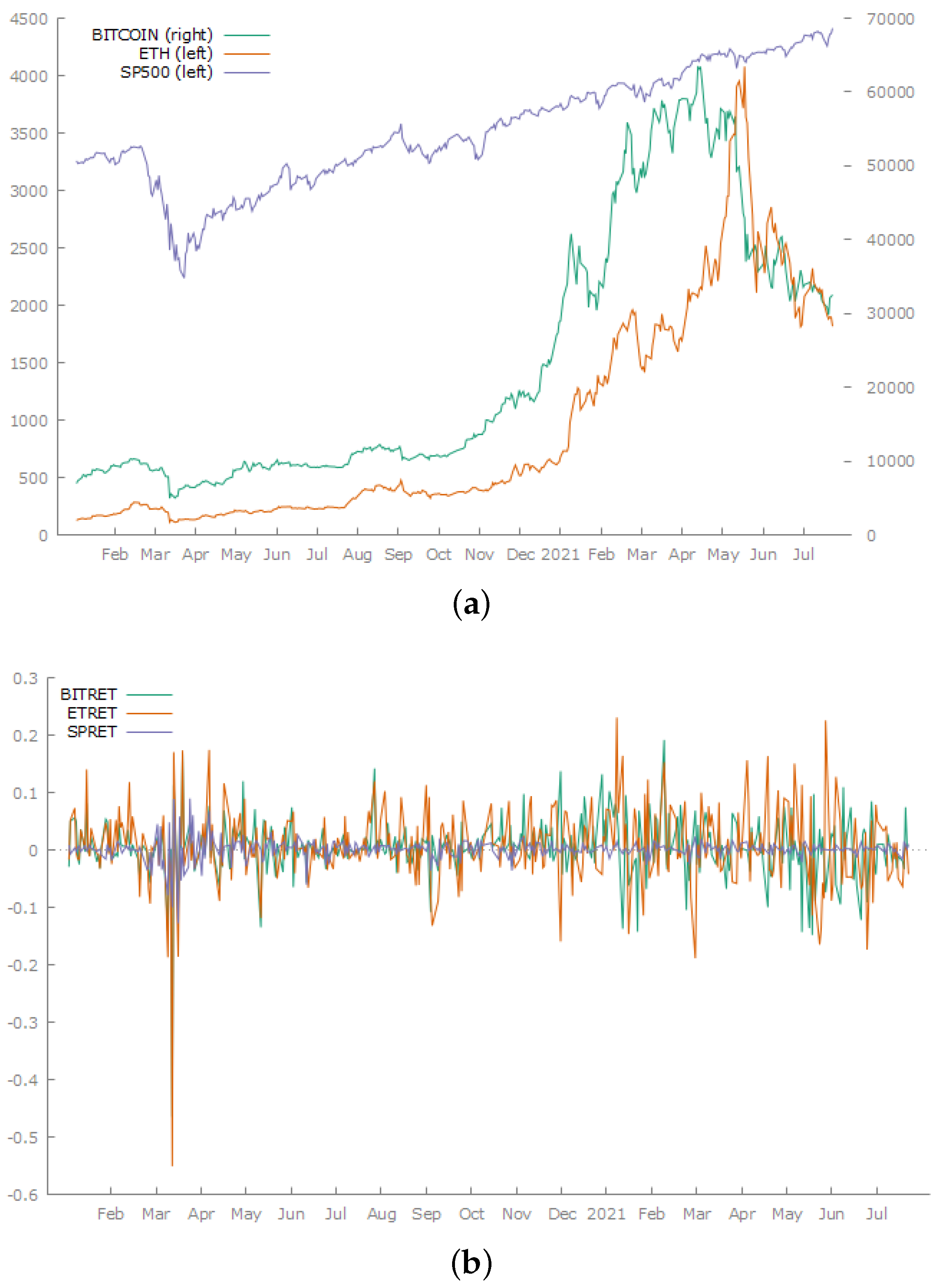
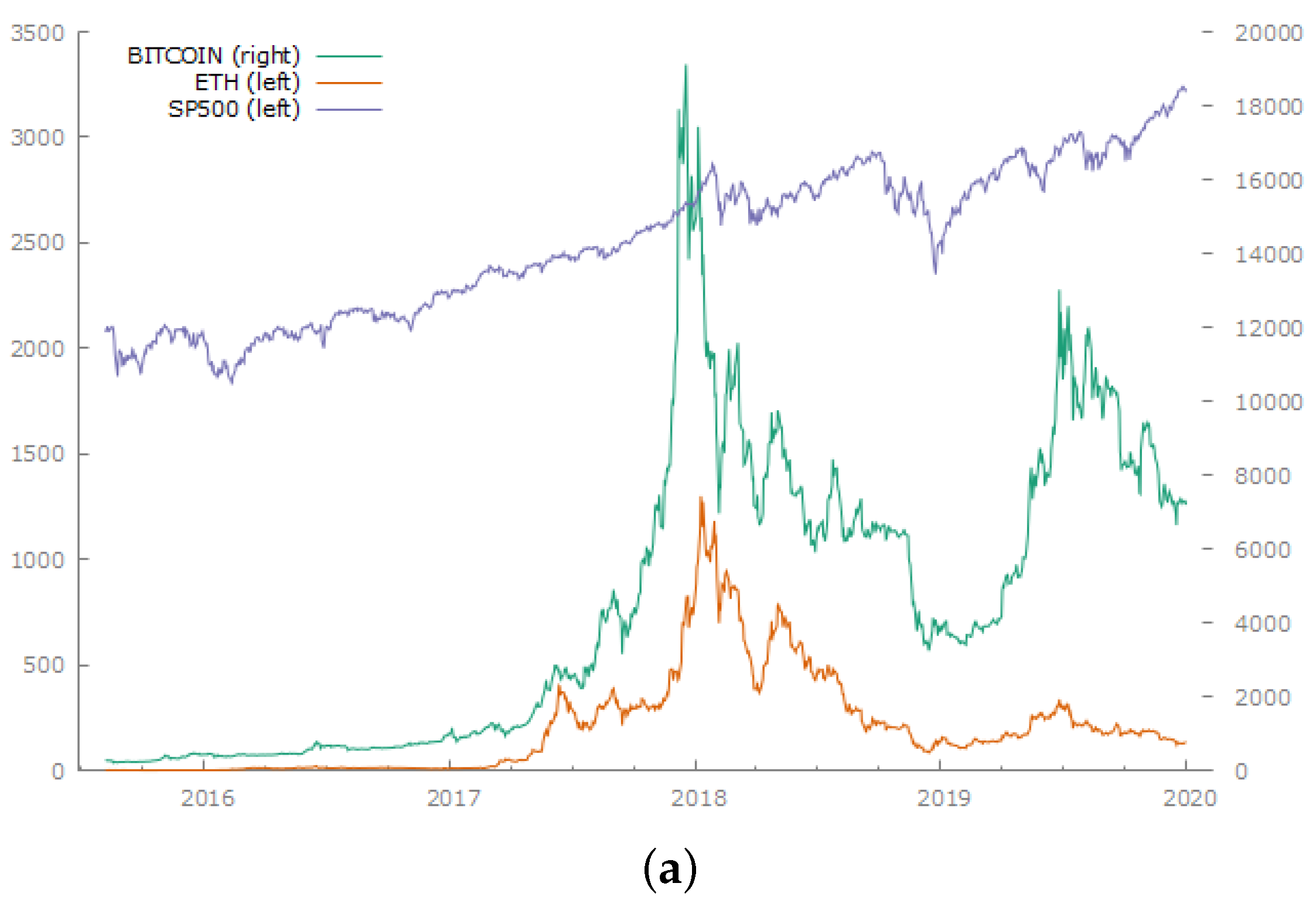
Graphs of the base price series and returns for the two sample time periods are shown in Figure 1 and Figure 2. The three base series all show evidence of trending behaviour in both periods. Plots of the price levels and returns on the series in the post-COVID-19 period are shown in Figure 2. Kwiatkowski et al. (1992) unit root tests, or more commonly termed KPSS tests, were undertaken on the levels of the series for both the pre- and post- COVID-19 samples, with the tests including a trend. The results are shown in Table 1. These show that all three series—Bitcoin, Ethereum and the S&P500 index in levels—reject the null hypothesis of stationarity at the 1 percent level. As a result, all of the analyses were performed on the continuously compounded return series.
Descriptive statistics for these series are presented in Table 2. It is apparent in Table 2 that the two cryptocurrencies have higher mean returns, a greater range of returns and considerably higher standard deviations in both periods than those of the S&P500 return series. All series display negative skewness and high kurtosis relative to a normal distribution, which would have a kurtosis of 3.
The results of the four different tests of conformance to a normal distribution are reported in the bottom panels, below the descriptive statistics, in Table 2. All four tests, namely, the Doornik–Hansen, Shapiro–Wilk, Lilliefors and Jarque–Bera tests reject the null hypothesis of a Gaussian distribution at greater than the one percent level for all three return series in both periods.
The Pearson correlation test is based on the assumption of linearity and conformance to a normal distribution. For this reason, the tests of association reported in this paper include non-parametric tests and non-linear measures of association.

3.2. Simple Tests of Correlation

The most straightforward test of the degree of correlation between the base return series is to estimate the Pearson correlation coefficient by running linear regressions. The results of these regression for the pre-COVID-19 period are shown in Table 3.
The regression in Table 3 reveal a significant correlation between BITRET and ETRET in the pre-COVID-19 period with a coefficient of 0.21, which is significant at the 1 percent level and an adjusted R-squared of 16.7. The Ramsey RESET test suggests that a linear relationship is not adequate. The addition of a squared ETRET term increases the adjusted R-square to 17.8 per cent and both the ETRET term and the squared ETRET term are significant at the 1 percent level.
The results of a regression of the returns on Bitcoin and Ethereum regressed on the S&P500 Index return during period 1 are shown in Table 4. It is notable that neither of these regressions have a significant slope coefficient on the S&P500 Index return. The F values of these regressions are not significant.
These results suggest that there are potential diversification benefits from investing in cryptocurrencies in Period 1, the pre-COVID-19 period, given that they are not significantly related to the return on the S&P500 Index return series on the basis of this metric.
These results are confirmed in Table 5 which reports the results of tests of the association between these three pairs of series in Period 1 using Kendall’s tau. The two cryptocurrencies are significantly related on these metrics, but neither are related to the return on the S&P500 Index returns in this pre-COVID-19 period.

3.3. Regression Analysis in Period 2

Table 6 shows the results of pairwise regressions of the returns on the three series in the post-COVID-19 period. Ramsey Reset Tests were performed on each regression specification and the results (not reported) suggested a non-linear relationship, so squared values of the independent variable were added to the regressions in all three cases. There was little change in the results across the two periods in the regression of BITRET and ETRET. The slopes coefficients were roughly 0.2 and adjusted R-squares were around 20 percent in both periods. The results of Kendall’s Tau measures of associated are reported in Table 7.
The notable change was in the relationship between the cryptocurrencies returns and the S&P500 Index returns. In the pre-COVID-19 period, the slope coefficients on SPRET were insignificant. In the second period, they became strongly positive and highly significant, though it must be borne in mind that the regressions include a significant coefficient on the squared term as well. This reflects a marked change in the relationship.

3.4. Non-Linear Non-Parametric Measures of Association in Period 1

The R library package kdecopula Nagler (2018) was used to fit copulas to paired return series using kernel density estimates. The package contains functions that are used to estimate the copula density from data. The only mandatory input is an n × 2 matrix of copula data, in effect, data with standard uniform margins.
Bouri et al. (2018) suggested three advantages for the use of copulas in assessing dependence. First, the copula method was designed to capture the complex and non-linear dependence structure of a multivariate distribution, enabling scrutiny of both tail dependence and the asymmetric dependence. Second, the marginal behaviour and the dependence structure are separated by the framework of copulas. This facilitates model specification and model estimation. Copulas can jointly combine different univariate models through their copula functions. Finally, copulas are invariant to increasing and continuous transformations; see Ning (2010).
The empirical application of copulas to financial time series of returns and the method for fitting marginal distributions was pioneered by Patton (2002) in his PhD thesis “Applications of Copula Theory in Financial Econometrics”, and a further description was provided in Patton (2006, pp. 536–37). He suggested the following models for the marginal distributions of a pair of return series:
X t = μ x + ϕ 1 x X t 1 + ε t
σ x , t 2 = ω x + β x σ x , t 1 2 + α x ε t 1 2
ν x σ x , t 2 ( ν x 2 ) . ε t i i d t v x .
A GARCH(1,1) model with a t-distribution was used to estimate the marginal distribution for the return series. This provided a first approximation, given that the package includes code to transform the data to uniform margins. (In the case of BITCOIN returns in period 1, an ARCH model was used, as GARCH failed to converge).
A further explanation of this approach, which features the use of a common but limited information set to model the marginal distributions, was provided by Patton (2013).
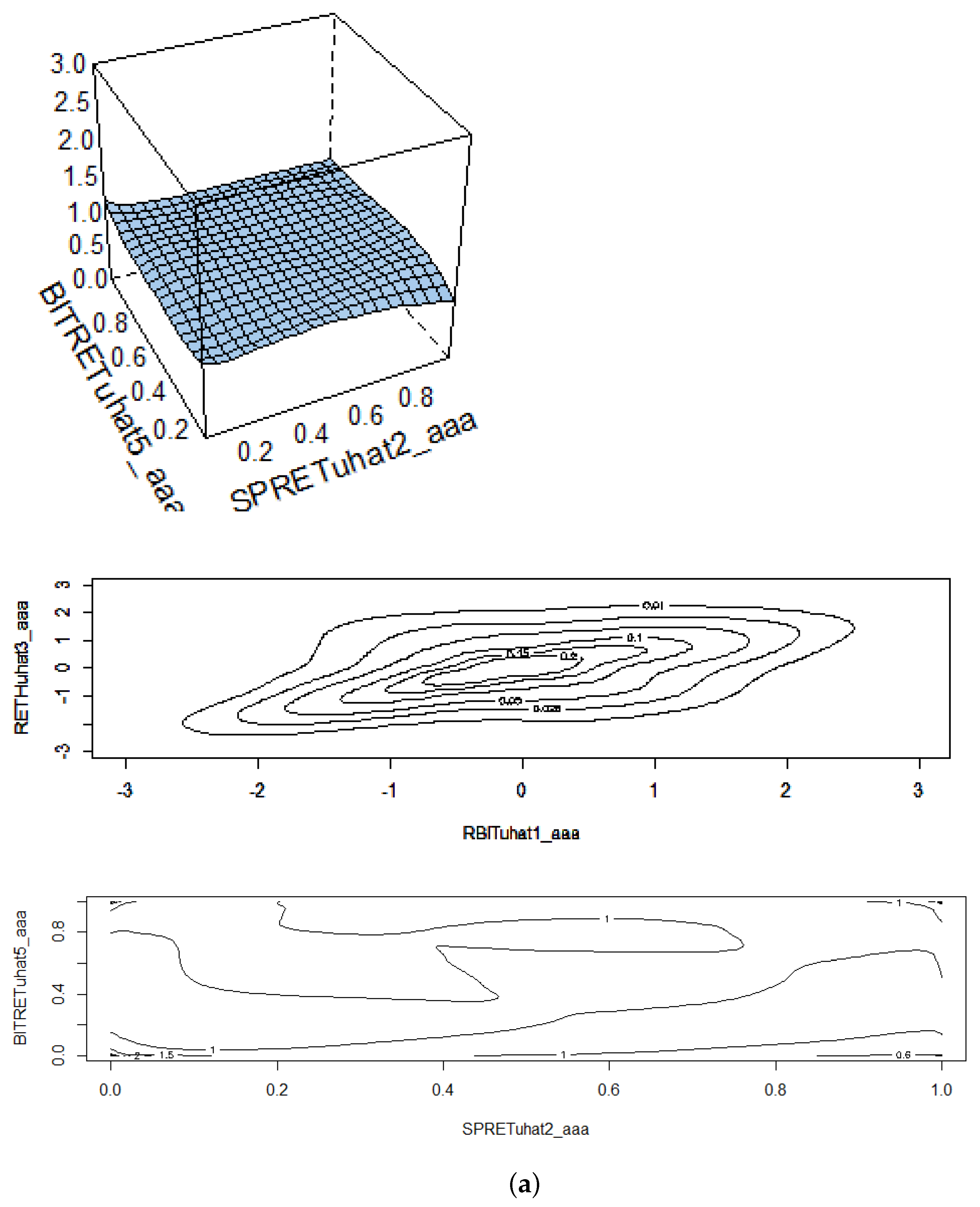
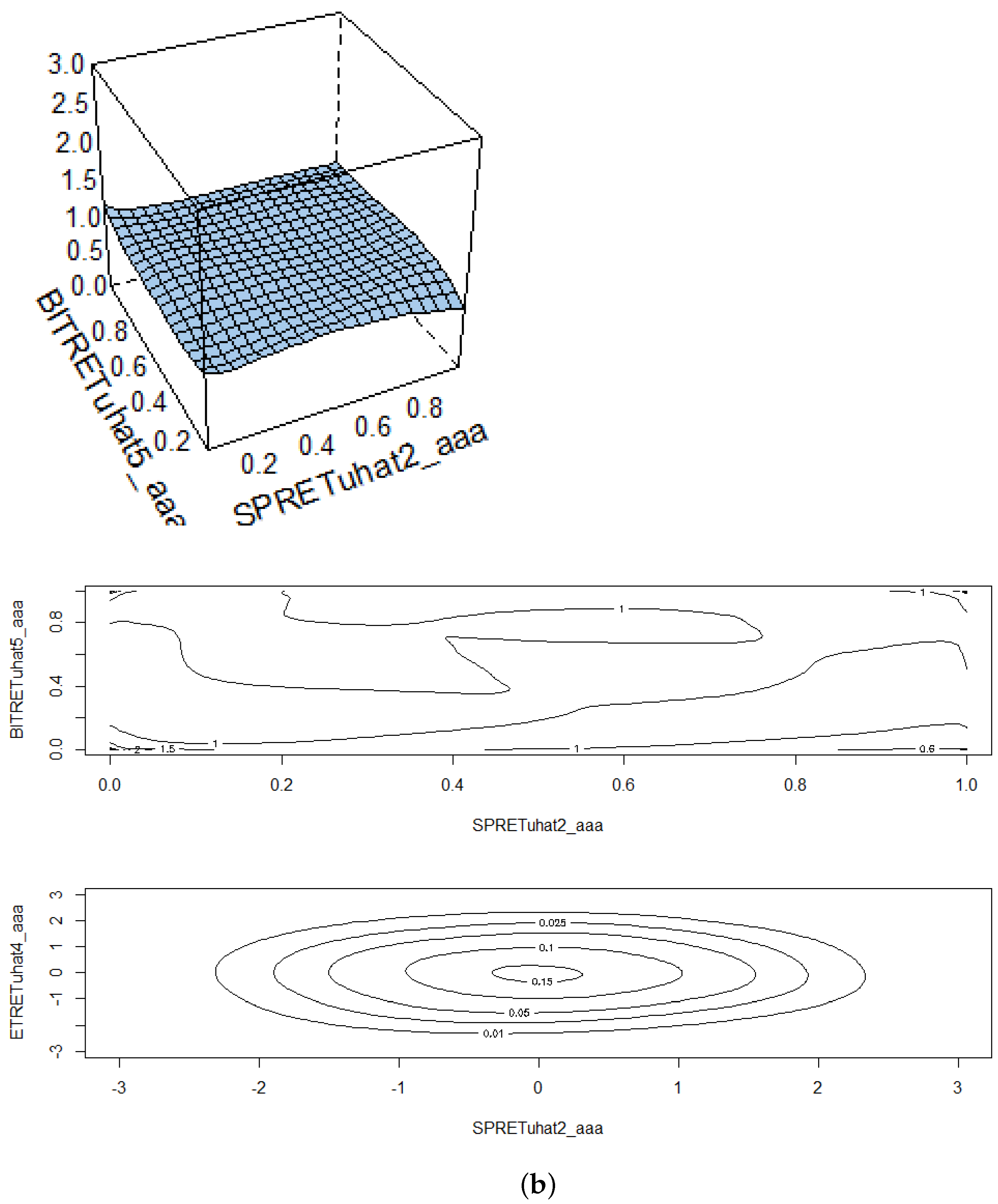
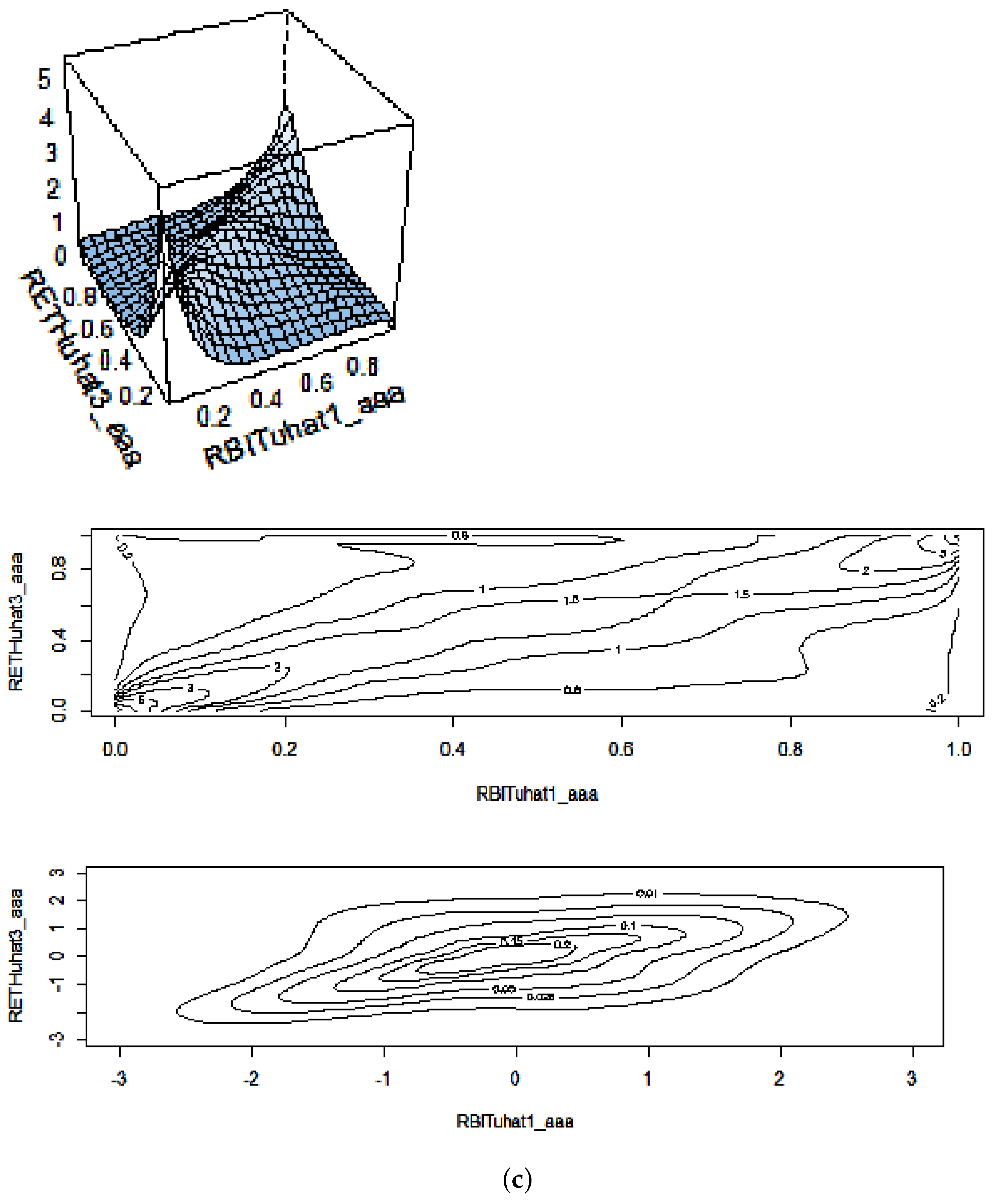
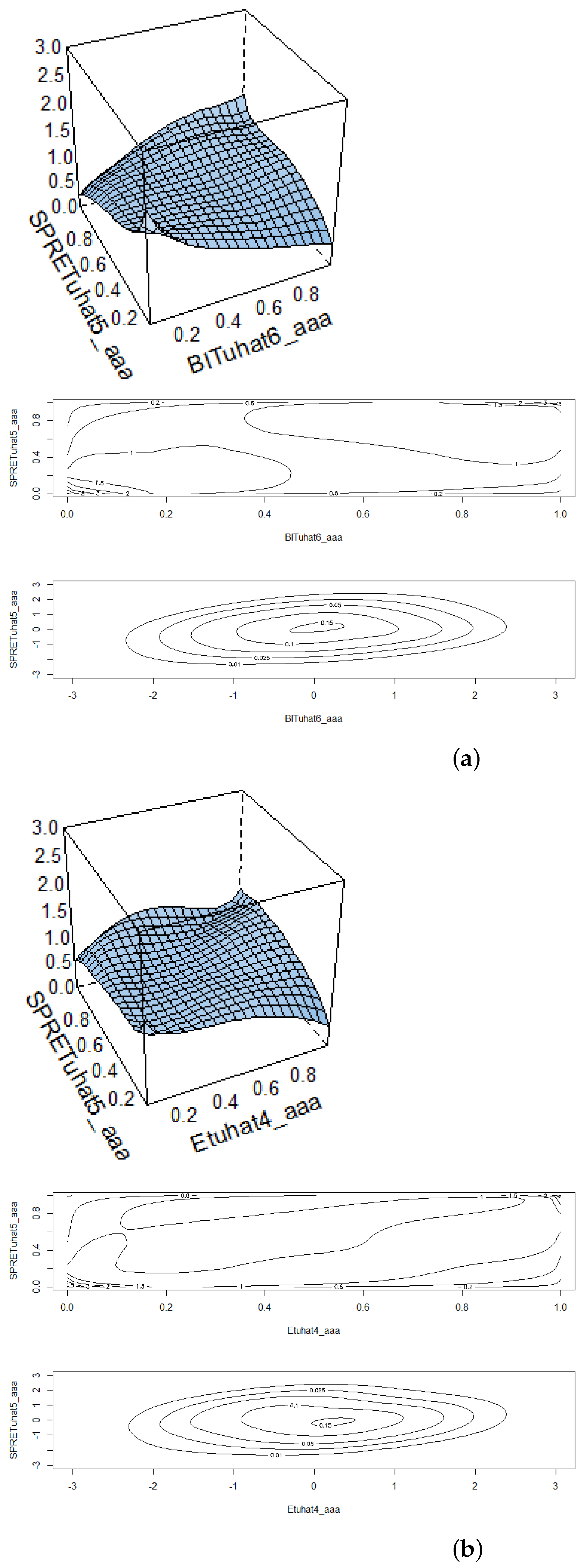
Table 8 provides a description of the results from fitting copulas to the paired series during the pre-COVID-19 period. The results are consistent with the previous estimates. There is a significant association between the returns on Bitcoin and Ethereum but a minimal association between the cryptocurrency returns and those on the S&P500 index. The diagrams in Panels A and C of Figure 3 show that the copula surfaces are fairly flat when cryptocurrencies are paired with S&P500 returns, and the contour density plots, particularly in panel C, are almost circular, depicting low levels of association. The first contour plot in each series in the figures shows the situation with uniform marginals.
A variety of measures of association are used in Table 8, and I shall comment briefly on the properties of some of the less frequently used ones. The Blomquist (1950) measure of association was developed for circumstances in which it would be valid under weak assumptions about the distribution of the data and easy to apply in practice. Blomquist (1950, p. 593) suggested that we consider two sample medians x ˜ and y ˜ . The cdf F ( x , y ) is assumed to have continuous marginal cdf’s F 1 ( x ) and F 2 ( y ) in order for the probability of obtaining two equal x-values or two equal y-values in the sample to be zero. Blomquist (1950) then divided the x , y -plane into four regions using the lines x = x ˜ and y = y ˜ . He then suggested that some information about the correlation between x and y can be obtained by the number of sample points, say n 1 , belonging to the first or third quadrants, compared with the number, say n 2 , belonging to the second or fourth quadrants. After suggesting a couple of further adjustments related to the total sample size, he then suggested that a measure of correlation can be defined as follows:
q = n 1 n 2 n 1 + n 2 = 2 n 1 n 1 + n 2 1 ( 1 q 1 ) .
Genest and Verret (2005, p. 521) noted that “testing for independence between two continuous random variables X and Y is an old but important problem that has been the object of much attention in the past century. Though a great deal of literature is available on the subject, test procedures based on Pearson’s correlation continue to be the most commonly used in practice. This is in spite of the well-known fact that this coefficient is merely a measure of linear association whose effectiveness, therefore, is questionable outside the normal paradigm, including for testing purposes”. They also suggest that all modern concepts of dependence and stochastic orderings are based on copulas, including Spearman’s rho, Kendall’s tau and other nonparametric alternatives to Pearson’s correlation coefficient.
Embrechts et al. (2002) pointed out that the dependence structure in a pair of variables ( X , Y ) with continuous distribution H and that margins F and G are best characterised by C , its unique underlying copula, implicitly defined on the unit square by the following:
H ( x , y ) = C { F ( x ) , G ( y ) } , x , y , R .
Modern concepts of dependence and stochastic orderings are based on copulas, which includes Spearman’s rho, Kendall’s tau and various nonparametric alternatives to Pearson’s correlation coefficient.
The copula of a random pair ( X , Y ) is unaffected by monotone increasing transformations of the margins. Given a random sample from H ( X 1 , Y 1 ) , , ( X n , Y n ) , the associated pairs of ranks ( R 1 , S 1 ) , , ( R n , S n ) are maximally invariant and can be used for a test of the hypothesis H 0 : H = F G , or equivalently, H 0 : C = Π , with Π ( μ , ν ) for all μ , ν ( 0 , 1 ) . A test based on kendall’s tau statistic can be written as
τ n = 2 n 2 n 1 i j n s i g n ( R i R j ) s i g n ( S i S j )
and can be used to reject the null hypothesis, for a large enough sample size n, where 3 n τ n / 2 > Φ 1 ( 0.975 ) = 1.96 , where Φ stands for the cumulative distribution function of a standard normal variable.
Another option based on Spearman’s rho is as follows:
ρ n = 3 n + 1 n 1 + 12 n 3 n i = 1 n R i S i ,
which leads to rejection of the null when the asymptotic p -value 2 Φ ( n ρ n ) of the two-sided test is too small.
Several other independence test statistics of the form
T n J = 1 n i = 1 n J R i n + 1 , S i n + 1
with specific score functions j , often perform as well as or better than standard parametric tests based on Pearson’s empirical correlation r n for various classes of alternatives.
Bhuchongkul (1964) demonstrated that the van der Waerden statistic, W n based on J ( μ , ν ) = Φ 1 ( μ ) Φ 1 ( ν ) , dominates r n for alternatives of the following form:
X i = X i + Δ Z i , Y i = Y i + Δ Z i ,
where X i , Y i and Z i are mutually independent random variables and Δ is a scalar.
Genest et al. (2010) discussed the close relationship between Spearman’s (1906) footrule Spearman (1906), which is a nonparametric measure of association, and Gini (1914) coefficient. The Spearman footrule can be written as follows:
φ n = 1 3 n 2 1 i = 1 n R i S i
whereas the indice de cograduazione semplice, introduced by Gini (1914), can be written as follows:
γ n = 1 [ n 2 / 2 ] i = 1 n { ( n + 1 R i ) S i R i S i } .
The last two measures, reported in Table 8 and Table 9, are based on information criteria. Let Xand Y be a pair of random variables. If their joint distribution is P ( X , Y ) and the marginal distributions are P X and P Y , the mutual information is described as follows:
I ( X , Y ) = D K L ( P ( X , Y ) P X P Y )
where D K L is the Kullback–Leibler divergence. Information theory was developed by Shannon (1948); Fano (1949) developed the concept of mutual information.
Hamdan and Tsokos (1971) discussed Linfoot (1957) informational measure of association between two random variables X and Y. The measure r 1 is based on the information gain r 0 in knowing that X and Y are mutually dependent with a given bivariate density function compared with the original knowledge that X and Y are statistically independent. Linfoot (1957) suggested that, if X and Y have bivariate normal distributions with correlation coefficient ρ , then r 0 = ( 1 / 2 ) l n ( 1 ρ 2 ) , which led to Linfoot (1957) suggestion that an informational measure ρ 1 of ρ be defined as follows:
r 1 = [ 1 e x p ( 2 ρ 0 ) ] 1 / 2
In the case of discrete random variables X and Y with bivariate probabilities p i j ( i = 1 , 2 , , s ; j = 1 , 2 , t ) and marginal probabilities p i = j p i j and p j = i p i j , r 0 take the following form:
r 0 = i j p i j l n p i j p i . p . j .
It is also the case that r 0 is equivalent to Kullback (1959) distance-like measure between the correlated bivariate distribution and the distribution under independence.
The various measures of association for the three combinations of the paired series returns, as reported in the lower panels of each section of Table 6, all tell a consistent story. The level of association between returns on Bitcoin and Ethereum is above 0.5, on the basis of the Spearman, Van de-Waerden and Linfoot metrics. For the definition of these measures used, see Nelsen (2006); Genest and Verret (2005); Joe (1989).
Genest and Verret (2005), in their assessment based on simulations, suggested that, whilst some dependence structures are easier to detect than others, the performance of rank tests can vary substantially from one set of alternatives to another. Pearson’s test seemed to be an acceptable procedure to use when the marginal distributions are normal but not necessarily when they are not. Van der Waerden’s test is likely to perform well whenever Pearson’s test performs well. It also has the additional advantage of being marginal-free. In terms of the limits of their simulation study, van der Waerden’s test seemed to hold a slight edge over Spearman’s and Kendall’s tests, which can be viewed as being essentially equivalent.
The results in Table 6 suggest that the degree of association between the two cryptocurrencies and the returns on the S&P500 index are virtually zero, as all of the measures bracket zero, either positively or negatively. This suggests that, in this period, investing in cryptocurrencies provides a potential diversification strategy. The concern is whether this remains the case when the market is subjected to the global shock of the pandemic? This is explored in the next sub-section.

3.5. Non-Linear Non-Parametric Measures of Association in Period 2

Table 9 reports the results of non-parametric copula density estimation in Period 2. The correlations between the returns on the two cryptocurrencies and those on the S&P500 Index appear to have increased markedly since the beginning of the COVID-19 pandemic. The estimates in Table 9 show that measures of association for BITRET and SPRET have increased in the case of the Kendall measure up to 0.15, whereas in the pre-COVID-19 period, it was −0.01, and similarly, the Spearman and Blomquist measures increased from −0.01 in both cases up to 0.23 and 0.15, respectively. In short, all of the metrics display a marked increase. The copula diagrams in Figure 4 confirm these changes.
Similarly, the estimates for ETRET and SPRET also show a marked increase. The Kendall and the Spearman measures stand at 0.08 and 0.11, whilst previously, they were 0.01 and 0.02, respectively. However, the correlations between the two cryptocurrencies appear to have diminished. In the pre-COVID-19 period, the Kendall and Spearman measures were 0.35 and 0.49, respectively; however, the the second period their values have fallen to 0.13 and 0.19, respectively. All of the measures for this pair in Table 7 record a decrease. However, Panel C in Figure 4 shows the copula between the two cryptocurrencies and suggests that they are still significantly associated.
In summary, these measures appear to show that the correlations between the returns on cryptocurrencies and those on the S&P500 Index show increases in times of crisis. This supports previous findings by Massoumi and Wu (2021, p. 1), who report that “NASDAQ daily return has the most similar density and co-dependence with Bitcoin daily return, generally, but after the COVID-19 outbreak in early 2020, even S&P500 daily return distribution is statistically closely dependent on, and indifferent from Bitcoin daily return”.

3.6. Generalised Measure of Correlation (GMC) Analysis

Table 10 presents the results of the GMC analysis in the two periods, pre- and post-COVID-19, and the results matrix reports the cause at the top of the columns and the response along the rows. If we begin with column 2 in Period 1, SPRET, the continuously compounded return on the S&P500 Index has a negative effect on the Bitcoin return, or a GMC of −0.55 and a negative effect on the Ethereum return of −0.73. The third column indicates that the Bitcoin return BITRET has a negative effect on SPRET of −0.57 and a positive effect on ETRET of 0.83. Finally, the fourth column under ETRET shows that the Ethereum return has a negative effect on SPRET of −0.47 and a positive effect on BITRET of 0.80.
Which way does causality run in Table 10? We can look at the coefficients above and below the diagonal in Table 10 and see that SPRET has an effect on BITRET of −0.56, but the effect of BITRET on SPRET is −0.47. Therefore, the stronger influence is from the S&P500 to Bitcoin rather than vice-versa, but the causality runs in both directions. Similarly, the effect of SPRET on ETRET is −0.73, whilst the effect of ETRET on SPRET is −0.47. Clearly, SPRET has the larger causal impact. Finally, we can see that BITRET has an 0.83 effect on ETRET, whilst ETRET has a 0.80 effect on BITRET. Therefore, Bitcoin has the slightly stronger causal influence when it is paired with Ethereum.
In the post-COVID-19 period 2 in Table 10, matters change dramatically. For a start, all of the GMC values have now become positive. This means that the relationship between the returns on the S&P500 Index returns, SPRET and the two cryptocurrencies, as represented by BITRET and ETRET, have increased to 0.69 and 0.68, respectively. Similarly, the influence of the cryptocurrencies on the S&P500 has become positive and greatly increased, as the last two entries in the row adjacent to SPRET are 0.68 and 0.81, respectively, which suggests that ETRET now has the largest impact on SPRET. The two cryptocurrencies have a large but slightly lower influence on one another. BITRET has a 0.77 GMC in relation to ETRET, whereas the influence of ETRET ON BITRET is now 0.72. These values are now slightly lower than the corresponding ones in the first period.
The most remarkable change is the switch in the signs of the relationships between the cryptocurrencies and the S&P500 from negative to positive, which suggests that they do not provide a strong diversification strategy in times of crisis.
4. Conclusions

The results of the tests of the measures of association between the returns on the S&P500 Index and the returns on these two cryptocurrencies, Bitcoin and Ethereum, in the the pre- and post-COVID-19 periods all tell a similar story, regardless of linear and parametric measures, or non-linear and non-parametric measures being adopted.
In the pre-COVID-19 period, the regression analysis suggests that there is a significant positive association between the two cryptocurrency returns series but no significant relationship with the S&P500 Index returns. Kendall’s tau tests of correlation provide a similar set of results. The results change in the post-COVID-19 period, and whilst the relationship between the two cryptocurrency returns series remains positive and significant, there is now a positive and significant relationship between the returns on both cryptocurrency returns series and the returns on the S&P500 Index. Kendall’s tau metric also suggests significant and positive relationships between all three series.
The non-parametric copula analysis of the relationship between the three pairs of series in the first period tells a similar story, suggesting that there is a significant association between the returns on Bitcoin and Ethereum but a minimal association between the cryptocurrency returns and those on the S&P500 index. In the second period, the results change notably, and the correlations between the returns on the two cryptocurrencies and those on the S&P500 Index appear to increase markedly.
The GMC analysis suggests a change in the sign of the relationship between the cryptocurrency returns and those on the S&P500 Index from negative to positive and a marked increase in their value. The direction of causality also appears to have switched and the strongest causal influence now appears to run from the returns on Ethereum to those on the S&P500 Index.
These changes are quite dramatic and suggest that cryptocurrencies in the form of Bitcoin and Etheureum do not provide a strong potential portfolio diversification tool, at least in the context of this particular crisis. This result is consistent with the findings of Massoumi and Wu (2021); Kristoufek (2020); Conlon et al. (2020); Lahmiri and Bekiros (2020); Grobys (2021).

Funding

This research received no external funding.

Institutional Review Board Statement

Not applicable.

Informed Consent Statement

Not applicable.

Data Availability Statement

The data was obtained from Yahoofinance and FRED, which are publicly available data sources. https://au.finance.yahoo.com/, https://fred.stlouisfed.org/, (accessed on 3 September 2021).

Acknowledgments

The author is grateful to the three anonymous reviewers for their helpful comments.

Conflicts of Interest

The author is not aware of any conflict of interest.

Note

1
I thank an anonymous reviewer for emphasising the importance of the explanation of this point.

References

  1. Akhtaruzzaman, Md, Ahmet Sensoy, and Shaen Corbet. 2020. The influence of bitcoin on portfolio diversification and design. Finance Research Letters 37: 101344. [Google Scholar] [CrossRef]
  2. Allen, David E., and Michael McAleer. 2020. Generalized Measures of Correlation for Asymmetry, Nonlinearity, and Beyond, Some Antecedents on Causality. Journal of the American Statistical Association 13: 1–11. [Google Scholar] [CrossRef]
  3. Allen, David E., and Vince Hooper. 2018. Generalized Correlation Measures of Causality and Forecasts of the VIX using Non-linear Models. Sustainability 10: 2695. [Google Scholar] [CrossRef] [Green Version]
  4. Baur, Dirk G., KiHoon Hong, and Adrian D. Lee. 2018. Bitcoin: Medium of exchange or speculative assets? Journal of International Financial Markets, Institutions and Money 54: 177–89. [Google Scholar] [CrossRef]
  5. Bhuchongkul, Subha. 1964. A class of nonparametric tests for independence in bivariate populations. The Annals of Mathematical Statistics 35: 138–49. [Google Scholar] [CrossRef]
  6. Blomqvist, Nils. 1950. On a measure of dependence between two random variables. The Annals of Mathematical Statistics 21: 593–600. [Google Scholar] [CrossRef]
  7. Bouri, Elie, Rangan Gupta, Chi Keung Lau, David Roubaud, and Shixuan Wang. 2018. Bitcoin and global financial stress: A copula-based approach to dependence and causality in the quantiles. The Quarterly Review of Economics and Finance 69: 297–307. [Google Scholar] [CrossRef] [Green Version]
  8. Bouri, Elie, Rangan Gupta, Aviral K. Tiwari, and David Roubaud. 2017a. Does Bitcoin hedge global uncertainty? Evidence from wavelet-based quantile-in-quantile regressions. Finance Research Letters 23: 87–95. [Google Scholar] [CrossRef] [Green Version]
  9. Bouri, Elie, Georges Azzi, and Anne Haubo Dyhrberg. 2017b. On the return-volatility relationship in the Bitcoin market around the price crash of 2013. Economics 11: 1–16. [Google Scholar] [CrossRef] [Green Version]
  10. Briere, Marie, Kim Oosterlinck, and Ariane Szafarz. 2015. Virtual currency, tangible return: Portfolio diversification with bitcoin. Journal of Asset Management 16: 365–73. [Google Scholar] [CrossRef]
  11. Chatterjee, Sourav. 2021. A new coefficient of correlation. Journal of the American Statistical Association 116: 2009–22. [Google Scholar] [CrossRef]
  12. Conlon, Thomas, Shaen Corbet, and Richard J. McGee. 2020. Are cryptocurrencies a safe haven for equity markets? An international perspective from the COVID-19 pandemic. Research in International Business and Finance 54: 101248. [Google Scholar] [CrossRef] [PubMed]
  13. Demir, Ender, Mehmet H. Bilgin, Gokhan Karabulut, and Asli Cansin Doker. 2020. The relationship between cryptocurrencies and COVID-19 pandemic. Eurasian Econonomic Review 10: 349–60. [Google Scholar] [CrossRef]
  14. Drozdz, Stanislaw, Jaroslaw Kwapien, Pawel Oswiecimka, Tomasz Stanisz, and Marcin Watorek. 2020. Complexity in economic and social systems: Cryptocurrency market at around COVID-19. Entropy 22: 1043. [Google Scholar] [CrossRef]
  15. Dyhrberg, Anne Haubo. 2016a. Bitcoin, gold and the dollar—A GARCH volatility analysis. Finance Research Letters 16: 85–92. [Google Scholar] [CrossRef] [Green Version]
  16. Dyhrberg, Anne Haubo. 2016b. Hedging capabilities of bitcoin. Is it the virtual gold? Finance Research Letters 16: 139–44. [Google Scholar] [CrossRef] [Green Version]
  17. Embrechts, Paul, Alistair J. McNeil, and Daniel Straumann. 2002. Correlation and dependence in risk management: Properties and pitfalls. In Risk Management: Value at Risk and Beyond. Edited by Michael A. H. Dempster. Cambridge: Cambridge University Press, pp. 176–223. [Google Scholar]
  18. Fano, Robert M. 1949. The Transmission of Information. Technical Report No. 65. Cambridge: Research Laboratory of Electronics at MIT. [Google Scholar]
  19. FRED. 2021. S&P Dow Jones Indices LLC. S&P 500 [SP500], Retrieved from FRED, Federal Reserve Bank of St. Louis. Available online: https://fred.stlouisfed.org/series/SP500 (accessed on 3 September 2021).
  20. Geneens, Gery, and Pierre Lafaye de Micheaux. 2019. The Hellinger Correlation. arXiv arXiv:1810.10276. [Google Scholar] [CrossRef]
  21. Genest, Christian, and Francois Verret. 2005. Locally most powerful rank tests of independence for copula models. Journal of Nonparametric Statistics 17: 521–39. [Google Scholar] [CrossRef]
  22. Genest, Christian, Johanna Neslehova, and Noomen Ben Ghorbal. 2010. Spearman’s footrule and Gini’s gamma: A review with complements. Journal of Nonparametric Statistics 22: 937–54. [Google Scholar] [CrossRef]
  23. Ghabri, Yosra, Khaled Guesmi, and Ahlem Zantour. 2021. Bitcoin and liquidity risk diversification. Finance Research Letters 40: 101679. [Google Scholar] [CrossRef]
  24. Gini, Corrado. 1914. L’Ammontare e la Composizione della Ricchezza delle Nazione. Torino: Bocca. [Google Scholar]
  25. Goodell, John W., and Stephane Goutte. 2021. Co-movement of COVID-19 and Bitcoin: Evidence from wavelet coherence analysis. Finance Research Letters 38: 101625. [Google Scholar] [CrossRef]
  26. Grobys, Klaus. 2021. When Bitcoin has the flu: On Bitcoin’s performance to hedge equity risk in the early wake of the COVID-19 outbreak. Applied Econonomic Letters 28: 860–65. [Google Scholar] [CrossRef]
  27. Guesmi, Khaled, Samir Saadi, Ilyes Abid, and Zied Ftiti. 2019. Portfolio diversification with virtual currency: Evidence from bitcoin. International Review of Financial Analysis 63: 431–37. [Google Scholar] [CrossRef]
  28. Hamdan, M. A., and Chris P. Tsokos. 1971. An Information Measure of Association in Contingency Tables. Information and Control 19: 174–79. [Google Scholar] [CrossRef] [Green Version]
  29. Ji, Quang, Elie Bouri, Rangan Gupta, and David Roubaud. 2017. Network Causality Structures among Bitcoin and Other Financial Assets: A Directed Acyclic Graph Approach. Report No 201729. Pretoria: Department of Economics, University of Pretoria. [Google Scholar]
  30. Joe, Harry. 1989. Relative entropy measures of multivariate dependence. Journal of the American Statistical Association 84: 157–64. [Google Scholar] [CrossRef]
  31. Kristoufek, Ladislav. 2020. Grandpa, grandpa, tell me the one about Bitcoin being a safe haven: New evidence from the COVID-19 pandemic. Frontiers in Physics 8: 296. [Google Scholar] [CrossRef]
  32. Kullback, Solomon. 1959. Information Theory and Statistics. New York: John Wiley and Sons. [Google Scholar]
  33. Kwiatkowski, Denis, Peter C. B. Phillips, Peter Schmidt, and Yongcheul Shin. 1992. Testing the null hypothesis of stationarity against the alternative of a unit root. Journal of Econometrics 54: 159–78. [Google Scholar] [CrossRef]
  34. Lahmiri, Salim, and Stelios Bekiros. 2020. The impact of COVID-19 pandemic upon stability and sequential irregularity of equity and cryptocurrency markets. Chaos, Solitons Fractals 138: 109936. [Google Scholar] [CrossRef]
  35. Li, Qi, and Jeffery S. Racine. 2007. Nonparametric Econometrics. Princeton: Princeton University Press. [Google Scholar]
  36. Linfoot, Edward H. 1957. An informational measure of correlation. Information and Control 1: 85–89. [Google Scholar] [CrossRef] [Green Version]
  37. Manavi, Seyed A., Gholamreza Jafari, Shahin Rouhani, and Marcel Ausloos. 2020. Demythifying the belief in cryptocurrencies decentralized aspects. A study of cryptocurrencies time cross-correlations with common currencies, commodities and financial indices. Physica A 556: 124759. [Google Scholar] [CrossRef]
  38. Massoumi, Esfandiar, and Xi Wu. 2021. Contrasting cryptocurrencies with other assets: Full distributions and the COVID Impact. Journal of Risk and Financial Management 14: 440. [Google Scholar] [CrossRef]
  39. Nadaraya, Elizbar A. 1964. On Estimating Regression. Theory of Probability and Its Applications 9: 141–42. [Google Scholar] [CrossRef]
  40. Nagler, Thomas. 2018. kdecopula: An R Package for the Kernel Estimation of Bivariate Copula Densities. Journal of Statistical Software 84: 1–22. [Google Scholar] [CrossRef] [Green Version]
  41. Nakamoto, Satoshi. 2008. Bitcoin: A Peer-to-Peer Electronic Cash System. Available online: Https://nakamotoinstitute.org/bitcoin (accessed on 19 September 2021).
  42. Nelsen, Rger B. 2006. An Introduction to Copulas. Springer Series in Statistics. New York: Springer, ISBN 0387286594. [Google Scholar]
  43. Ning, Cathy. 2010. Dependence structure between the equity market and the foreign exchange market—A copula approach. Journal of International Money and Finance 29: 743–59. [Google Scholar] [CrossRef]
  44. Patton, Andrew J. 2002. Applications of Copula Theory in Financial Econometrics. Ph.D thesis, University of California, San Diego, CA, USA. [Google Scholar]
  45. Patton, Andrew J. 2006. Modelling Asymmmetric Exchange Rate Dependence. International Economic Review 47: 527–56. [Google Scholar] [CrossRef]
  46. Patton, Andrew J. 2013. Copula Methods for Forecasting Multivariate Time Series. In Handbook of Economic Forecasting. Edited by Graham Elliott and Aalan Timmermann. Amsterdam: Springer. [Google Scholar]
  47. Qarni, Md O., and Saihb Gulzar. 2021. Portfolio diversification benefits of alternative currency investment in Bitcoin and foreign exchange markets. Financial Innovation 7: 1–37. [Google Scholar] [CrossRef]
  48. Salmon, Felix. 2009. Recipe for disaster: The formula that killed Wall Street. Wired Magazine, February 23. [Google Scholar]
  49. Shahzad, Syed J. H., Elie Bouri, David Roubaud, and Ladislav Kristoufek. 2020. Safe haven, hedge and diversification for G7 stock markets: Gold versus bitcoin. Economic Modelling 87: 212–24. [Google Scholar] [CrossRef]
  50. Shannon, Claude E. 1948. A Mathematical Theory of Communication. Bell System Technical Journal 27: 379–23, 623–56. [Google Scholar] [CrossRef] [Green Version]
  51. Sklar, Abe. 1959. Fonctions de Repartition an Dimensions et Leurs Marges. Paris: Universite Paris 8, Vincennes-Saint-Denis. [Google Scholar]
  52. Spearman, Charles. 1906. Footrule for Measuring Correlation. The British Journal of Psychiatry 2: 89–108. [Google Scholar] [CrossRef]
  53. Vinod, Hrishikesh D. 2014. Matrix Algebra Topics in Statistics and Economics Using R. In Handbook of Statistics: Computational Statistics with R. Edited by Marepalli B. Rao and C. R. Rao. New York: Elsevier Science, vol. 34, chp. 4. pp. 143–76. [Google Scholar]
  54. Vinod, Hrishikesh D. 2016. generalCorr: Generalized Correlations and Initial Causal Path, Fordham University, New York, R Package Version 1.1.2, 2018, Has 3 Vignettes. Available online: https://CRAN.R-project.org/package=generalCorr (accessed on 3 September 2021).
  55. Vinod, Hrishikesh D. 2017. Generalized Correlation and Kernel Causality with Applications in Development Economics. Communications in Statistics—Simulation and Computation 46: 4513–34. [Google Scholar] [CrossRef]
  56. Vinod, Hrishikesh D. 2020. generalCorr: Generalized Correlations and Various Causal Paths, R Package Version 1.1.8. Available online: https://CRAN.R-project.org/package=generalCorr (accessed on 3 September 2021).
  57. Yule, George Udney. 1897. On the Significance of Bravais Formule for Regression, in the case of skew correlation. Proceedings of The Royal Society London 60: 477–89. [Google Scholar]
  58. Watorek Marcin, Stanislaw Drozdz, Jaroslaw Kwapien, Ludovico Minati, Pauwel O’swiecimka, and Marek Stanuszek. 2021. Multiscale characteristics of the emerging global cryptocurrency market. Physics Reports 901: 1–82. [Google Scholar] [CrossRef]
  59. Watson, Geoffrey S. 1964. Smooth regression analysis. Sankhyā: The Indian Journal of Statistics, Series A 26: 359–72. [Google Scholar]
  60. Zheng, Shurong, Ning-Zhong Shi, and Zhenjun Zhang. 2012. Generalized measures of correlation for asymmetry, nonlinearity, and beyond. Journal of the American Statistical Association 107: 1239–52. [Google Scholar] [CrossRef]
Figure 1. Plots of the series pre-COVID-19. (a) Plot price series levels pre-COVID-19. (b) Plot of returns pre-COVID-19.
Jrfm 15 00103 g001aJrfm 15 00103 g001b
Figure 2. Plots of the series post-COVID-19. (a) Price series levels post-COVID-19. (b) Plot of returns post-COVID-19.
Jrfm 15 00103 g002
Figure 3. Kernel Density Estimates of Copula fitted to Ajusted Return Series Period 1 Pre-COVID-19. (a) Panel A: BITRET and SPRET. (b) Panel B: ETRET and SPRET. (c) Panel C: BITRET and ETRET.
Jrfm 15 00103 g003aJrfm 15 00103 g003bJrfm 15 00103 g003c
Figure 4. Kernel density estimates of copula fitted to adjusted return series Period 2 COVID-19. (a) BITRET and SPRET. (b) ETRET and SPRET. (c) BITRET and ETRET.
Jrfm 15 00103 g004aJrfm 15 00103 g004b
Table 1. KPSS unit root tests including trend on levels of the series pre- and post-COVID-19.
Pre-COVID-19 Period 1107 Observations
SeriesTest StatisticCritical Value 1%Significance
Bitcoin0.9065870.218p-value < 0.01
Ethereum1.985510.218p-value < 0.01
S&P500 Index0.892120.218p-value < 0.01
Post-COVID-19 Period 388 Observations
SeriesTest StatisticCritical Value 1%Significance
Bitcoin0.5706690.217p-value < 0.01
Ethereum1.0070.217p-value < 0.01
S&P500 Index0.8192120.217p-value < 0.01
Table 2. Sample period descriptive statistics return series and tests of normality.
Pre-COVID-19
VariableMeanMedianMinimumMaximumStandard DeviationSkewnessKurtosis
BitRet0.00306440.0028579−0.238740.225120.045864−0.0665294.3715
EthRet0.0037798−0.00076875−1.36430.509690.088035−2.786855.437
SPRet0.000402150.00055609−0.0418430.0484030.0086027−0.566054.11
Doornik-HansenShapiro-WilkLillieforsJarque-Bera
BitRet384.5 ***0.918 ***0.115 ***881.5 ***
EthRet3174.1 ***0.779 ***0.126 ***143,056 ***
SPRet23,591.6 ***0.5134 ***0.185 ***5,267,300 ***
Post-COVID-19 Sample Period Descriptive Statistics Return Series
VariableMeanMedianMinimumMaximumStandard DeviationSkewnessKurtosis
BitRet0.00411520.0034694−0.464730.191530.051090−2.016318.759
EthRet0.00676570.0040564−0.550730.230700.065380−1.480113.968
SPRet0.000802430.0017851−0.127650.0896830.018271−1.011612.402
Doornik-HansenShapiro-WilkLillieforsJarque-Bera
BitRet261.5 ***0.854 ***0.121 ***5952 ***
EthRet285.5 ***0.888 ***0.098 ***3295.9 ***
SPRet379.8 ***0.811 ***0.144 ***2552.7 ***
Note: *** Indicates significance at 1 percent level.
Table 3. Return Regressions Pre-COVID-19.
BITRET Regression on ETRET
OLS, using observations 2015-08-10–2019-12-31 (T = 1106)
Dependent variable: BITRET
CoefficientStd. Errort-ratiop-value
const0.002257180.001259611.7920.0734
ETRET0.2135610.014301314.930.0000
Mean dependent var0.003064S.D. dependent var0.045864
Sum squared resid1.933742S.E. of regression0.041852
R 2 0.168043Adjusted R 2 0.167290
F ( 1 ,   1104 ) 222.9924p-value(F)4.58 × 10 46
ρ ^ 0.042830Durbin–Watson1.886082
RESET test for specification—
   Null hypothesis: specification is adequate
   Test statistic: F ( 2 ,   1102 ) = 54.6266
   with p-value = P( F ( 2 ,   1102 ) > 54.6266) = 2.39666 × 10 23
Regression with Squared ETRET added
OLS, using observations 2015-08-10–2019-12-31 (T = 1106)
Dependent variable: BITRET
CoefficientStd. Errort-ratiop-value
const0.001471660.001266931.1620.2457
ETRET0.2351290.015214715.450.0000
sq_ETRET0.09075000.02290853.9610.0001
Mean dependent var0.003064S.D. dependent var0.045864
Sum squared resid1.906616S.E. of regression0.041576
R 2 0.179714Adjusted R 2 0.178227
F ( 2 , 1103 ) 120.8264p-value(F)3.56 × 10 48
ρ ^ 0.056203Durbin–Watson1.882833
Table 4. Cryptocurrency returns regressed on S&P500 Index returns Period 1.
BITRET Regressed on S&P500 Index Returns
OLS, using observations 2015-08-10–2019-12-31 (T = 1106)
Dependent variable: BITRET
CoefficientStd. Errort-ratiop-value
const0.003065750.001379752.2220.0265
SPRET−0.01273360.107227−0.11880.9055
Mean dependent var0.003064S.D. dependent var0.045864
Sum squared resid2.324301S.E. of regression0.045884
R 2 0.000013Adjusted R 2 −0.000893
F ( 1 ,   1104 ) 0.014102p-value(F)0.905492
ρ ^ 0.020015Durbin–Watson1.958382
RESET test for specification—
   Null hypothesis: specification is adequate
   Test statistic: F ( 2 ,   1102 ) = 0.94016
   with p-value = P( F ( 2 ,   1102 ) > 0.94016) = 0.390878
Regression of ETRET on S&P500 Index Return Period 1
OLS, using observations 2015-08-10–2019-12-31 (T = 1106)
Dependent variable: ETRET
CoefficientStd. Errort-ratiop-value
const0.003783850.002648401.4290.1534
SPRET−0.03805040.205821−0.18490.8534
Mean dependent var0.003780S.D. dependent var0.088035
Sum squared resid8.563712S.E. of regression0.088074
R 2 0.000031Adjusted R 2 −0.000875
F ( 1 ,   1104 ) 0.034177p-value(F)0.853364
ρ ^ 0.006020Durbin–Watson1.769479
RESET test for specification—
   Null hypothesis: specification is adequate
   Test statistic: F ( 2 ,   1102 ) = 1.04091
   with p-value = P( F ( 2 ,   1102 ) > 1.04091) = 0.353479
Table 5. Kendall’s tau measure of association among the return series in Period 1.
Paired SeriesKendall’s TauZ-ScoreTwo-Tailed Probability
BITRET and SPRET−0.009084140.6897120.4904
ETRET and SPRET0.013849590.6897120.4904
ETRET and BITRET0.3550833417.68520.0000
Table 6. Return regressions post-COVID-19.
BITRET Regression on ETRET
OLS, using observations 2020-01-02–2021-07-23 (T = 388)
Dependent variable: BITRET
CoefficientStd. Errort-ratiop-value
const0.007372110.002371193.1090.0020
ETRET0.2007770.03651305.4990.0000
sq_ETRET−1.071010.142508−7.5150.0000
Mean dependent var0.004115S.D. dependent var0.051090
Sum squared resid0.759745S.E. of regression0.044423
R 2 0.247872Adjusted R 2 0.243965
F ( 2 ,   385 ) 63.44057p-value(F)1.54 × 10 24
ρ ^ −0.074587Durbin–Watson2.147612
Return Regressions Post-COVID-19 BITRET Regression on SPRET
OLS, using observations 2020-01-02–2021-07-23 (T = 388)
Dependent variable: BITRET
CoefficientStd. Errort-ratiop-value
const0.005581600.002481222.2500.0250
SPRET0.9150620.1347566.7900.0000
sq_SPRET−6.596781.95763−3.3700.0008
Mean dependent var0.004115S.D. dependent var0.051090
Sum squared resid0.849030S.E. of regression0.046960
R 2 0.159483Adjusted R 2 0.155116
F ( 2 ,   385 ) 36.52566p-value(F)2.99 × 10 15
ρ ^ −0.060347Durbin–Watson2.118522
Regression of ETRET on SPRET Period 2 COVID-19
OLS, using observations 2020-01-02–2021-07-23 (T = 388)
Dependent variable: ETRET
CoefficientStd. Errort-ratiop-value
const0.009243890.003224522.8670.0044
SPRET0.9675870.1751265.5250.0000
sq_SPRET−9.756242.54408−3.8350.0001
Mean dependent var0.006766S.D. dependent var0.065380
Sum squared resid1.433917S.E. of regression0.061028
R 2 0.133186Adjusted R 2 0.128683
F ( 2 ,   385 ) 29.57768p-value(F)1.12 × 10 12
ρ ^ 0.008506Durbin–Watson1.979712
Table 7. Kendall’s tau measure of association between the the return series in Period 2.
Paired SeriesKendall’s TauZ-ScoreTwo-Tailed Probability
BITRET and SPRET0.145768404.287220.000
ETRET and SPRET0.059751191.757120.079
ETRET and BITRET0.110178753.240390.001
Table 8. Non-parametric copula-estimation-transformed returns Period 1.
BITRET and SPRET
Kernel Copula Density estimate tau = −0.0065
Observations = 1107Method: Transformation local likelihood, log-quadratic (nearest-neighbor)
Band width alpha = 0.5363016
logLik: 3.27AIC: 20.48cAIC: 20.83BIC: 88.12
Effective number of parameters: 13.5
Kendall −0.0065Spearman −0.0096Blomquist −0.0109Gini −0.0102
vd_waerden −0.0008minfo 0.00165linfoot 0.0574
ETRET and SPRET
Kernel Copula Density estimate tau=0.014
Observations = 1107Method: Transformation local likelihood, log-quadratic (nearest-neighbor)
Bandwidth: alpha = 0.5363016
logLik: 4.49AIC: 18.21cAIC: 18.57BIC: 86.33
Effective number of parameters: 13.6
Kendall 0.0143Spearman 0.0218Blomquist 0.0113Gini 0.0151
vd_waerden 0.0270minfo 0.0016Linfoot 0.0567
BITRET and ETRET
Kernel Copula Density estimate tau=0.35
Observations = 1608Method: Transformation local likelihood, log-quadratic (nearest-neighbor)
Bandwidth: alpha = 0.1920285
logLik: 378.95AIC: −699.29cAIC: −698.16BIC: −541.55
Effective number of parameters: 29.3
Kendall 0.3535Spearman 0.4873Blomqvist 0.3535gini 0.4007
vd_waerden 0.5027minfo 0.2137linfoot 0.5897
Table 9. Non-parametric Copula estimation-transformed returns Period 2.
BITRET and SPRET
Kernel Copula Density estimate tau = 0.15
Observations = 388Method: Transformation local likelihood, log-quadratic (nearest-neighbor)
Bandwidth: alpha = 0.5803161
logLik: 18.98AIC: −15.07cAIC: −14.31BIC: 30.26
Effective number of parameters: 11.24
Kendall 0.1546Spearman 0.2316Blomquist 0.1450Gini 0.1758
Van der Waerden 0.2536Minfo 0.0390Linfoot 0.2738
ETRET and SPRET
Kernel Copula Density estimate tau = 0.075
Observations = 388Method: Transformation local likelihood, log-quadratic (nearest-neighbor)
Band width alpha = 0.5886832
LogLik: 15.49AIC: −7.52cAIC: −6.72BIC: 38.93
Effective number of parameters: 11.73
Kendall 0.0753Spearman 0.1125Blomquist 0.0491Gini 0.0768
Van der Waerden 0.1457Minfo 0.0203Linfoot 0.1995
BITRET and ETRET
Kernel Copula Density estimate tau = 0.013
Observations = 388Method: Transformation local likelihood, log-quadratic (nearest-neighbor)
Bandwidth: alpha = 0.4297086
logLik: 39.05AIC: −47.77cAIC: −46.45BIC: 12.29
Effective number of parameters: 15.16
Kendall 0.1301Spearman 0.1886Blomquist 0.1217Gini 0.1493
Van der Waerden 0.2167Minfo 0.0559Linfoot 0.3253
Table 10. GMC analysis.
Period 1: Pre-COVID-19
SPRETBITRETETRET
SPRET1.000−0.4542502−0.4695773
BITRET−0.55638811.0000.8003115
ETRET−0.72997760.83243651.000
Period 2: Post-COVID-19
SPRETBITRETETRET
SPRET1.0000.67584050.8140017
BITRET0.68983181.0000.7194903
ETRET0.68402180.76719891.000
Publisher’s Note: MDPI stays neutral with regard to jurisdictional claims in published maps and institutional affiliations.