Article

The Dynamic Relationship between Investor Attention and Stock Market Volatility: International Evidence

by
Imene Ben El Hadj Said
1 and
Skander Slim
2,*
1
LaREMFiQ, University of Sousse, Sousse 4000, Tunisia
2
Dubai Business School, University of Dubai, Dubai 14143, United Arab Emirates
*
Author to whom correspondence should be addressed.
J. Risk Financial Manag. 2022, 15(2), 66; https://doi.org/10.3390/jrfm15020066
Submission received: 4 November 2021 / Revised: 24 January 2022 / Accepted: 26 January 2022 / Published: 1 February 2022
(This article belongs to the Special Issue Mathematical and Empirical Finance)

Abstract

:
This paper investigates the role of investor attention in forecasting realized volatility for fourteen international stock markets, by means of Google Trends data, over the sample period January 2004 through November 2021. We devise an augmented Empirical Similarity model that combines three volatility components, defined over different time horizons, using the similarity measure between lagged Google search queries and volatility. Results show that investor attention positively affects future volatility in the short-run. The effect of investor attention is likely to reverse in the long-run, consistently with the price pressure hypothesis. The proposed model demonstrates important gains in terms of volatility forecast accuracy and outperforms highly competitive models.

1. Introduction

It has been commonly assumed that investors behave rationally. A long strand of literature provides evidence that this assumption is unrealistic and that investors behavior is, indeed, prone to psychological biases. Several studies show that taking into account psychological features in financial analysis can explain several anomalies observed in stock markets.
The present study belongs to a growing literature on the importance of behavioral aspects in explaining stock market movements. Particularly, this paper focuses on limited attention, one of the most prevalent psychological biases. Investors are limited in their ability to optimally allocate attention across various sources of information (Kahneman 1973). Most importantly, previous studies contend that attention allocation is a key determinant of investor’s trading decisions (Simon 1955). For instance, Barber and Odean (2008) find evidence that investors are net buyers of attention-grabbing stocks. Peng and Xiong (2006) suggest that attention could explain under-reaction and overreaction to news, which causes prices to swing away from their fundamental values. Besides, Andrei and Hasler (2014) argue that a high level of attention accelerates the transmission of news into stock prices, which leads to a higher level of volatility. Thus, examining investor attention can shed light on a variety of observations in stock markets. In this context, two challenging problems arise: (i) selecting an accurate measure of investor attention and (ii) determining the appropriate approach to study the link between investor attention and stock market volatility.
A rich literature highlights the importance of online search intensity in exploring the trading activity (see, e.g., Bank et al. 2011; Ekinci and Bulut 2021; Joseph et al. 2011; Klemola et al. 2016; Padungsaksawasdi et al. 2019, among others). Crowds of internet users daily search for specific terms through web search engines. One of the most popular search engines is Google.1 Da et al. (2011) argue that searching for a stock in Google provides a clear indication of investor’s interest in that stock. Interestingly, they use the Google Volume Index (GVI) to gauge the attention of retail investors. In an intriguing study, Hamid and Heiden (2015) note that the movements of the GVI for the term “dow” are well aligned with that of the DJIA volatility. Based on this observation, they extend the Empirical Similarity (ES) model, developed by Lieberman (2012), in order to examine the link between investor attention and the volatility of the DJIA index. By allowing the autoregressive coefficient to depend on the similarity between past GVI and volatility, their model is shown to improve the accuracy of volatility forecasts.
The aim of present paper is to investigate the role of investor attention in forecasting volatility for 14 international stock markets, by means of GVI. This paper extends the study of Hamid and Heiden (2015) in several ways. First, we employ a larger dataset and examine whether the findings of Hamid and Heiden (2015) hold for a broader set of international stock markets covering the geographical regions of America (Brazil, Mexico and U.S.), Europe (Belgium, France, Germany, Netherlands, Spain, Switzerland and U.K.), Asia (China, India, Japan) and Australia, over a time window of about 18 years of weekly observations spanning from 5 January 2004 to 26 November 2021. Second, we propose an augmented Empirical Similarity model, which we dub HAR-ES. Our model is based on the similarity measure between lagged GVI and three volatility components, defined over different time horizons, of the Heterogeneous Autoregressive (HAR) model (Corsi 2009). In addition to the attractiveness of the HAR model, which has been proven to account for the main stylized facts of volatility and to achieve higher predictive performance than traditional volatility models, Golosnoy et al. (2014) show that combining the HAR components using the ES approach leads to systematic improvements over the HAR model. While Golosnoy et al. (2014) use the similarity between past values of volatility, we employ the similarity between two different variables, namely GVI and volatility. Therefore, the HAR-ES accounts not only for the dynamics of GVI and realized volatility but also the heterogeneous beliefs among investors via heterogeneous volatility components. More specifically, our model incorporates time-varying coefficients that account for the dynamics of both GVI and volatility. Thus, we expect our model to show rapid adjustment to changes in stock market volatility.
Our methodology is summarized as follows. First, we examine causal relationships between GVI and volatility by means of Granger causality test. Second, in order to investigate the sign and timing of the relationships between investor attention and volatility, we estimate a bivariate VAR model. Finally, the forecasting performance of our predictive regressions is compared by using the modified Diebold and Mariano (1995) test and the Model Confidence Set approach (Hansen et al. 2011) based on noise-robust loss functions. Our main results point to the superiority of the HAR-ES model over benchmark volatility forecasting models for almost all markets. More importantly, we find that our model outperforms the ES model proposed by Hamid and Heiden (2015).
The rest of the paper is structured as follows. Section 2 presents related literature. Section 3 introduces the econometric models. Section 4 describes the data and discusses the empirical results. Section 5 concludes.

2. Literature Review

Prior research shows that understanding investors behavior is quintessential in financial analysis. Researchers have explored various psychological aspects and studied their impacts on the behavior of investors. One of the major psychological biases is limited attention. The psychology of attention is an active field of research in cognitive psychology. The general conclusion emerging from research in this area is that attention is a scare cognitive resource (Kahneman 1973). A relevant strand in the literature stemming from the “price pressure hypothesis” (Barber and Odean 2008) states that investors do not face the same search problem when deciding whether to buy or sell stocks. Individual investors are net buyers of attention-attracting stocks (Grullon et al. 2004). Barber and Odean (2008) point out that investors have to choose among a large set of stocks when buying, which involves a search activity that requires attention, whereas when winding up their positions, investors sell stocks that they already own, thereby assuming that they do not often sell short. More importantly, the authors provide evidence that attention-driven buying induces short-term positive price pressure, most markedly for retail investors.
A large number of studies suggest that examining investor attention can shed light on a variety of observations in stock markets (e.g., DellaVigna and Pollet 2009; Hasler and Ornthanalai 2018; Mondria and Quintana-Domeque 2013; Seasholes and Wu 2007). In their study, Peng and Xiong (2006) showed that investors display category-learning behavior. They argue that, given the vast amount of information, investors mostly focus on both market-level and sector-level information rather than on firm-specific information. In addition, Hou et al. (2009) showed that a high level of attention leads to an overreaction, in which case investors are likely to buy recent winners and sell losers. Hence, they suggest that attention-driven overreaction may explain the price momentum effect. Moreover, Hou et al. (2009) point out that when attention decreases, investors may under-weight earnings announcement. Consequently, earnings news will not be fully integrated into prices, which leads to a stronger stock price underreaction. Thus, this lack of attention may justify post-earnings announcement drift. In the same vein, Hirshleifer et al. (2009) proposed the “investor distraction hypothesis” according to which the arrival of many competing announcements distracts investor attention from earnings news, resulting in a weaker stock price reaction, lower trading volume and a stronger post-announcement drift.
Analyzing investor behavior using the Internet has gained momentum in recent years. The number of Internet users has increased massively all over the world. In this context, Da et al. (2011) suggest that online search intensity may reveal the attention of investors to stock markets. They examined the link between investor attention and stock returns using the GVI of ticker symbols for a sample of the Russell 3000 constituent stocks. The availability of the GVI has expanded the scope of research and has been applied in various fields of study (see, e.g., Carneiro and Mylonakis 2009; Choi and Varian 2012; Ginsberg et al. 2009; Guzman 2011; Vosen and Schmidt 2011; Yang et al. 2015). In their study, Da et al. (2011) tested and confirmed the price pressure hypothesis. They found that a large abnormal search volume induces higher prices (i.e., positive price pressure) in the subsequent two weeks and a price reversal within the year. Da et al. (2011) emphasized that this proxy reflects the attention of individual investors rather than that of institutional investors, who use more advanced tools to collect information, such as Reuters and Bloomberg terminals. Within the GARCH framework, Vlastakis and Markellos (2012) showed that the volume of Google search queries positively affects stock market volatility. Andrei and Hasler (2014) found that investor attention drives future volatility, though the reverse causality is not supported. Within a VAR framework, Vozlyublennaia (2014) found strong evidence that investor attention affects future returns in the short-term. Nonetheless, the link between volatility and investor attention is less pronounced. In addition, past returns have a significant long-lasting impact on investor attention. The most noteworthy result to emerge from Vozlyublennaia (2014) is that past performance of certain market indices is a key determinant of the impact of the previous level of attention on future returns and volatility. Klemola et al. (2016) used the GVI to explain changes in S&P 500 index returns. They measured investor attention during up-market periods using the search frequency for the terms “bull market” and “market rally”. Additionally, they used the GVI for “bear market” and “market crash” to gauge investor attention during market downturns. They found evidence that pessimistic search terms predict lower stock returns and optimistic search terms, predict higher stock returns. Chen (2017) documented a negative effect of investor attention on stock returns for a sample of 67 countries. The effect was found to be more pronounced in developed countries and tends to be weaker (stronger) during low (high) sentiment periods. Wen et al. (2019) used the search frequency from the Baidu index as a proxy of investor attention, and documented a negative relationship between investor attention and expected stock price crash risk in China.
Though several studies have shown that investor attention significantly affects stock market movements, a very limited number of research papers have investigated its role in predicting future volatility. Using panel data regression models, Kim et al. (2019) showed that the predictive power of Google search is stronger than its contemporary explanatory power for both volatility and trading volume, although there exists no relation between GVI and stock returns in the Norwegian market. Dimpfl and Jank (2016) investigated the link between GVI and the volatility of the DJIA index. They found that augmenting the Autoregressive (AR) and the Heterogeneous Autoregressive (HAR) models with the Google component significantly improves the forecasting accuracy of volatility. However, Hamid and Heiden (2015) showed that simply adding the GVI variable into the HAR model worsens the fit and does not improve the forecasting power. Interestingly, they showed that the ES approach is more suitable than standard models for studying the link between volatility and investor attention. The authors conjecture that past volatility determines the impact of the previous level of investor attention on future volatility. Their model demonstrates important gains in terms of volatility forecast accuracy by using a similarity measure between RV and GVI. More recently, Wang et al. (2021) investigated the impact of investors attention to the COVID-19 pandemic on stock market volatility. Their findings indicate that the expected component of investor attention is more informative about the stock market dynamics than its unexpected counterpart.
To date, the methodology of Hamid and Heiden (2015) has only been applied to the DJIA index. The present paper aims to test the results of Hamid and Heiden (2015) on a broader set of stock markets. Most subtly, we provide new insights into the relationship between investor attention and stock market volatility by proposing an augmented empirical similarity model. The empirical similarity approach has been successfully applied in volatility modeling and forecasting (e.g., Golosnoy et al. 2014; Hamid 2015; Hamid and Heiden 2015). Hamid and Heiden (2015) showed that an AR(1) model with a time-varying coefficient that varies with the similarity between volatility and GVI is highly advantageous to examine the link between investor attention and market volatility. In the present paper, we merely combine the HAR model with the ES approach using the similarity between the GVI and volatility.

3. Econometric Models

This section describes the realized models employed to examine the relationship between volatility and investor attention. Accordingly, we present our empirical similarity specification (HAR-ES) which allows GVI to affect short, medium and long-term realized volatility components, differently. For the sake of comparison, we also present the empirical similarity approach in Hamid and Heiden (2015) and several benchmark volatility models augmented with GVI.

3.1. The Empirical Similarity Model

Hamid and Heiden (2015) propose a volatility modeling framework based on the similarity between two different variables, namely, volatility and GVI, rather than the similarity between the same variable over time (Lieberman 2012). These two variables are similar in the sense that they evolve in the same way. The ES model is given by:
R V i , t = ω 0 + exp ω 1 ( G i , t 1 R V i , t 1 ) β t ( G i , t 1 , R V i , t 1 , w 1 ) R V i , t 1 + ϵ i , t
where R V i , t is volatility of index i in week t, G i , t represents Google data of the ith index, ω = ( ω 0 , ω 1 ) R is a vector of unknown parameters and ϵ i , t i . i . d N ( 0 , σ 2 ) . β t ( G i , t 1 , R V i , t 1 , w 1 ) is the similarity function. It is real-valued, non-negative and non-stochastic function. The ES model can be estimated using MLE. This model is grounded on the observation that past volatility determines the impact of previous level of investor attention on future volatility. If the similarity function β t ( G i , t 1 , R V i , t 1 , w 1 ) is constant t , the model in Equation (1) is simply reduced to an AR(1) model:
R V i , t = ω 0 + ω 1 R V i , t 1 + ϵ i , t
We also augment the AR(1) model with a Google component of lag ( t 1 ) and examine whether simply adding the Google variable significantly improves the accuracy of volatility forecasts. We denote this model by AR-G, where G refers to Google data. The AR-G model is specified as follows:
R V i , t = ω 0 + ω 1 R V i , t 1 + g 1 G i , t 1 + ϵ i , t

3.2. The Heterogeneous Autoregressive (HAR) Model

The HAR model has been widely used due to its simplicity and intuitive structure and has been proven to achieve higher predictive performance than traditional volatility models (Andersen et al. 2007; Corsi 2009; Corsi and Reno 2012). The HAR model accommodates an additive cascade of heterogeneous volatility components over different time horizons and allows to mimic the long memory feature of volatility as well as other stylized facts of financial data. The HAR model is specified as follows:
R V i , t = ω 0 + ω 1 R V i , t 1 ( s ) + ω 2 R V i , t 1 ( m ) + ω 3 R V i , t 1 ( l ) + ϵ i , t
where R V i , t is weekly realized volatility of index i, R V i , t 1 ( s ) is the short-term component, R V i , t 1 ( m ) and R V i , t 1 ( l ) are the average RV during the previous 5 and 22 weeks, respectively, and ϵ i , t i . i . d ( 0 , σ 2 ) .
Our study focuses on the role of investor attention in explaining the dynamics of stock market volatility. Thus, we augment the standard HAR model with the Google component. The HAR-G is specified as follows:
R V i , t = ω 0 + ω 1 R V i , t 1 ( s ) + ω 2 R V i , t 1 ( m ) + ω 3 R V i , t 1 ( l ) + g 1 G i , t 1 + ϵ i , t

3.3. The Empirical Similarity Approach with the HAR Components

Inspired by the study of Golosnoy et al. (2014); Hamid and Heiden (2015), we propose an augmented ES model to examine the relationship between volatility and investor attention. The HAR-ES model is specified as follows:
R V i , t = θ G i , t 1 , R V i , t 1 ( s ) R V i , t 1 ( s ) + θ G i , t 1 , R V i , t 1 ( m ) R V i , t 1 ( m ) + θ G i , t 1 , R V i , t 1 ( l ) R V i , t 1 ( l ) θ G i , t 1 , R V i , t 1 ( s ) + θ G i , t 1 , R V i , t 1 ( m ) + θ G i , t 1 , R V i , t 1 ( l ) + ϵ i , t ,
with
θ G i , t 1 , R V i , t 1 ( s ) = exp ω 1 ( G i , t 1 R V i , t 1 ( s ) ) , θ G i , t 1 , R V i , t 1 ( m ) = exp ω 2 ( G i , t 1 R V i , t 1 ( m ) ) , θ G i , t 1 , R V i , t 1 ( l ) = exp ω 3 ( G i , t 1 R V i , t 1 ( l ) ) ,
where θ [ . , . ] is the similarity function. The HAR-ES model is simply a weighting average of three volatility components (short, medium and long-term), where the weights are determined via the similarity between lagged Google data and the previous levels of volatility. The basic idea behind our model is that volatility varies with investor attention, depending on the previous levels of volatility. Thus, the HAR-ES specification can be viewed as an HAR model with time-varying coefficients. It can be rewritten as follows:
R V i , t = ϕ G i , t 1 , R V i , t 1 ( s ) R V i , t 1 ( s ) + ϕ G i , t 1 , R V i , t 1 ( m ) R V i , t 1 ( m ) + ϕ G i , t 1 , R V i , t 1 ( l ) R V i , t 1 ( l ) + ϵ i , t
where ϕ [ . , . ] is normalized relative empirical similarity with ϕ G i , t 1 , R V i , t 1 ( s ) + ϕ G i , t 1 , R V i , t 1 ( m ) + ϕ G i , t 1 , R V i , t 1 ( l ) 1 .
Interestingly, the HAR-ES model captures not only the dynamics of GVI and RV, but also the heterogeneous beliefs among investors via heterogeneous volatility components. We expect the parameter ω 1 to be positive; a decrease in difference between G i , t 1 and R V i , t 1 ( s ) (i.e., more similarity) increases the weight of the short-term component. Inversely, we expect the parameters ω 2 and ω 3 to be negative. An increase in difference between G i , t 1 and R V i , t 1 ( m ) ( R V i , t 1 ( l ) ) (i.e., less similarity) increases the effect of the mid-term (long-term) component, since future prices are expected to converge to their fundamental values owing to their mean-reverting behavior.

4. Empirical Analysis

4.1. Data Description

The empirical analysis is carried out on 14 major stock markets around the globe. The data cover 14 stock market indices including the AEX index (Netherlands), All Ordinaries (Australia), BEL 20 (Belgium), Bovespa (Brazil), BSE Sensex (India), CAC 40 (France), DAX 30 (Germany), DJIA (U.S.), FTSE 100 (U.K.), Hang Seng (China), IBEX 35 (Spain), IPC (Mexico), Nikkei 225 (Japan) and SMI (Switzerland). We use the Realized Volatility measure based on 5-minute intraday returns with subsampling. The Realized Volatility series are obtained from the Oxford-Man Institute’s Quantitative Finance Realized Library (Heber et al. 2009).
Our proxy for investor attention is the Google Volume Index (GVI) provided by Google Trends.2 Google Trends is a publicly available tool of Google Inc. Google Trends records how many searches have been done for a specific search query. Nonetheless, Google Trends does not provide absolute numbers, but rather relative search values. Indeed, the volume of search term is divided by the total number of search queries for the time and location selected. After this normalization, data are scaled by the highest relative search volume and multiplied by 100. The choice of keywords to identify a stock market index is critical. Obviously, investors are likely to use short search terms in order to gather information. Table 1 presents the stock market indices and the corresponding search terms used in our study. Note that for the BSE Sensex index, we use the keyword “sensex”. The search term “bse sensex” is also popular but has lower search volume than that of “sensex”. Besides, for the Hang Seng index, we use the search term “hang seng index “ rather than “hang seng” in order to avoid noise in the search volume because the keyword “hang seng” may also refer to the Hang Seng bank. Furthermore, we do not use the keyword “hsi” because this search term has lower search volume in China. Our dataset spans from 5 January 2004 to 26 November 2021 which yields a sample of 934 weekly observations for each market. As Google Trends restricts the access to 5-year windows of weekly data, we can not simply merge those windows due to normalization and standardization. We propose a method that allows us to merge windows into a single time series (see Appendix A). Figure 1 plots the Realized Volatility and the Google Trends data for our sample indices. Figure 1 shows that volatility movements are homogeneous across market indices and during major events such as the subprime crisis in 2008 and the COVID-19 outbreak in March 2020, which effect on world economy and financial markets is still unfolding. That is, investors pay more attention to stock markets during turmoil periods. The movements in GVI seem to be well aligned with volatility for all but five market indices (All Ordinaries, Hang Seng, IBEX 35, IPC and Nikkei 225). Remarkably, movements in the DJIA volatility and GVI are perfectly similar. This similarity, also reported in Hamid and Heiden (2015), points out the usefulness of Google data in explaining stock market dynamics.
Table 2 reports summary statistics of RV and GVI series for our sample. The statistics provide strong support for the widely-documented stylized facts of Realized Volatility. The distribution of volatility is heavily skewed to the right and exhibits a high kurtosis. The IBEX 35 index has the lowest skewness (5.12) and kurtosis (38.69), while the All ordinaries index has the highest skewness (10.43) and the Hang Seng index exhibits the highest kurtosis (153.49). The RV series exhibit a high degree of autocorrelation ranging from 0.47 (for BSE Sensex) to 0.79 (for All Ordinaries). Additionally, the unit root tests indicate that all series are stationary. The Google series exhibit similar statistical features. More importantly, we find that market volatility is positively correlated with the volume of Google search queries, which is in line with previous results reported in the literature.

4.2. Lead–Lag Relationship between Volatility and Investor Attention

In order to examine causal relationships between RV and GVI, we conduct Granger causality analysis for each stock market index. Then, we use a bivariate VAR model to gauge the sign and timing of the effects between investor attention and volatility. The model is given by
X i , t = ϕ 0 + ϕ 1 X i , t 1 + + ϕ k X i , t k + ϵ i , t
where the vector X i , t contains the realized volatility R V i , t and the corresponding Google data G i , t for the ith market index, and ϵ i , t is a white noise process. We estimate the model with a lag parameter k of up to 10, and we finally select a lag length based on information criteria.
Results of the Granger causality test, reported in Table 3, reveal that there exists a significant bidirectional causality between RV and GVI for eleven indices. We interpret the causal relationship running from GVI to RV as follows. An increase in investor attention indicates that more information is processed by the market. Consequently, retail investors create a short-term price pressure which results in a higher level of stock market volatility. Inversely, when investor attention is low (i.e., information demand is low) retail investors are likely to be losing interest in the stock market resulting in lower participation and lower volatility. As suggested by Andrei and Hasler (2014) and Vozlyublennaia (2014), it is less likely that past volatility causes future investor attention. Indeed, if that were the case, then investor attention would not be useful in predicting future market movements. However, previous levels of volatility may affect the impact of past attention on future volatility. Results indicate that there exists a unidirectional causality running from RV to GVI for Hang Seng and IBEX 35. Surprisingly, we find no Granger causality between RV and GVI for the IPC index. Overall, we find no evidence that current attention causes future volatility for the Hang Seng, IPC and IBEX 35 indices. There are several possible explanations for these findings. Since the GVI reflects the attention of individual investors (Da et al. 2011), the proportion of individual investors in the group of countries including China, Mexico and Spain may be lower than that in the other countries. Another possible explanation is that information asymmetry among investors may be less pronounced in this country group. In such cases, retail investors demand less information. According to StatCounter3, the most popular search engine in China is Baidu. This fact may also explain the absence of a causal relationship running from GVI to RV for the Hang Seng index.
We estimate a bivariate VAR model following Vozlyublennaia (2014) and Hamid and Heiden (2015). Table 4 reports VAR estimation results for each stock market index. Results show that the volume of Google search queries positively affects future RV in the short-run, since the first lag of GVI is significantly positive for all indices. Our findings also indicate that an increased investor attention creates a short-term price pressure leading to a higher level of volatility, in line with previous studies including Vlastakis and Markellos (2012), Vozlyublennaia (2014), Hamid and Heiden (2015) and Dimpfl and Jank (2016).
It is worth mentioning that the first lag of GVI is insignificant for Nikkei 225, IPC, IBEX 35 and FTSE 100. This may be attributed to a relatively low coverage for those indices, which results in a delayed reaction to the stock market. Moreover, the effect of investor attention on volatility is likely to reverse in the long-run for major indices, consistently with the price pressure hypothesis. Indeed, an increase in the level of investor attention results in higher stock market participation. Once they have participated, investors devote less attention to the stock market due to diminishing perceived uncertainty, even though the level of volatility is still high. Table 4 further shows that past volatility affects current investor attention. However, we observe both positive and negative effects of lagged RV on current Google search volume across stock markets.

4.3. Estimation Results

In this Section, we report the estimation results of the AR, AR-G, ES, HAR, HAR-G and HAR-ES models. As shown in Table 5, the Google component included in the AR-G model is significantly positive for all indices, except for the FTSE 100, Hang Seng and IBEX 35 indices, for which we find insignificant coefficients. Thus, our results are consistent with previous findings, which show that stock market volatility is positively affected by investor attention in the short-term. The magnitude of the coefficient g 1 is the highest for the AEX index. As regards the ES model, the coefficient w 1 is significantly positive for all indices. For positive w 1 ’s values, a decreasing distance between lagged GVI and RV (i.e., more similarity) increases the weight assigned to lagged volatility.
As shown in Figure 2, the coefficient β t is highly dynamic during volatile periods with a sharp increase in its level when stock market volatility rises. Subsequently, when volatility declines, the parameter β t decreases, reaching values lower than 1. During low volatility periods, the coefficient β t is relatively stable. This pattern is economically consistent with the main idea behind the ES model in Hamid and Heiden (2015). That is, we hardly expect a significant change in stock market volatility compared to its recent level in cases of high investor attention and volatility. The same holds true when both investor attention and volatility are low. In the former situation, the coefficient β t rises sharply, putting more weight on the recent level of volatility. Subsequently, investor attention is likely to decrease, owing to lower participation of investors in the stock market, and the parameter β t will decrease sharply. In the latter situation, the parameter β t will remain constant, thereby reducing the ES model to an AR(1).
Results further show that the Google component included into the HAR-G model is significantly positive for six indices. Concerning the HAR-ES model, we find that the short-term component is significantly positive for six markets; significantly negative for FTSE 100, DJIA and IPC; and insignificant for the other markets. It is noteworthy that the insignificance of the coefficient w 1 does not mean that the short-term component is irrelevant in explaining stock market volatility. It rather indicates that its explanatory power is transmitted via the other components, owing to normalization (see Equation (6)). Positive w 1 ’s values indicate more similarity between G i , t 1 and R V i , t 1 ( s ) which increases the weight assigned to the short-term component. Indeed, when investor attention and volatility are both high, investors create a short-term price pressure, which implies a higher level of volatility. Otherwise, if both investor attention and volatility are low, we expect that the level of future volatility will remain constant. Hence, this similarity increases the weight assigned to the previous level of RV. Besides, we find that the coefficient w 2 is significantly negative for seven indices; significantly positive for Nikkei 225, IPC and Hang Seng; and insignificant for BEL 20, BSE Sensex, DJIA and FTSE 100. For the long-term component, the coefficient w 3 is significantly negative for eight indices; and significantly positive for Hang Seng and IPC. Negative w 3 ’s values indicate that an increasing distance between G i , t 1 and R V i , t 1 ( l ) (i.e., less similarity) increases the weight assigned to the long-term component, since future prices are expected to converge to their fundamental values. It is worth mentioning that the sign of the coefficients w 2 and w 3 is significantly positive in few cases, though we expected negative coefficients. This may be due to less similarity between the two variables for some stock markets.
In order to illustrate typical patterns arising from our ES-based model, Figure 3 displays the variations over time of the coefficient estimates and parameters for the AEX index. The three coefficients of the HAR-ES model are relatively stable during low-volatility periods and highly dynamic during high volatility phases. The short-term component ( p h i 1 ) tends to increase when RV rises, putting more weight on the previous level of volatility, and decreases subsequently when RV declines. Inversely, the mid-term ( p h i 2 ) and long-term ( p h i 3 ) components decrease when RV surges and then rise when RV decreases, since prices are expected to return to their fundamental values. Hence, these parameters show rapid adaptation to changes in stock market volatility, which makes the HAR-ES model fairly suitable for volatility modeling. Note that for some indices, we find the same pattern for the short-term and mid-term components but opposite patterns for the long-term component, which could have been caused either by the relatively low frequency of our data or the larger distance between RV and GVI for some indices. After showing that investor attention significantly affects future stock market volatility, it is worth investigating whether GVI improves volatility forecasts.

4.4. Volatility Forecast Evaluation

In this Section, we empirically assess the forecasting power of each model. In a rolling window setup, we re-estimate our models on a weekly basis. We evaluate the forecasting performance of predictive models for our sample indices including those for which we find little evidence that GVI affects future RV, since our forecasting exercise produces updated parameter estimates. First, we compare the one-step-ahead forecasting accuracy using the MAE, the MSE and the QLIKE loss functions. These loss functions are widely used for the ranking of competing volatility forecasts. The MSE and the QLIKE are homogeneous and robust to the presence of noise in the volatility proxy (Patton 2011). The MAE and MSE are symmetric while the QLIKE is an asymmetric loss function that penalizes under-prediction more heavily. Table 6 reports the average losses for competing models, relative to the HAR-ES losses.
Results show that the HAR-ES model has the lowest MAE for all market indices. Regarding the MSE and QLIKE, the HAR-ES yields the lowest forecasting error for twelve indices. As regards to the QLIKE, the ES model has the lowest average loss only for Bovespa and DJIA. Besides, our findings indicate that simply adding the GVI variable to the AR and HAR models worsens the fit and does not improve the forecasting performance.
We further employ the modified Diebold-Mariano (DM) test for pairwise comparison of the forecasting error across the different models. Patton and Sheppard (2009) find that the power of the DM test is higher when using the QLIKE than when using other loss functions. Therefore, we run the DM test using the QLIKE loss function. The results are reported in Table 7. Not surprisingly, the t-statistics in the comparison between the HAR and AR models are significantly negative for four out of fourteen markets. Results show that simply adding the Google component to the AR and HAR models does not improve forecasting accuracy. Indeed, we find that the t-statistics are significantly negative for almost all indices, when considering the pairs AR vs. AR-G and HAR vs. HAR-G. Both ES and AR provide equal forecasting performance as evidenced by the insignificant t-statistics in most of the cases. When comparing between the ES and AR-G models, we find that the ES model is significantly superior to the AR-G for four indices, while the latter outperforms the former only for the BSE Sensex. The ES model outperforms the HAR model only for the SMI index, while the HAR model yields more accurate forecasts than the ES model for four markets. Results further show that the pairs HAR-ES vs. AR and HAR-ES vs. AR-G have significant and negative t-statistics. Hence, the HAR-ES model is significantly superior to the AR and AR-G models. Additionally, the DM test confirms the superiority of the HAR-ES over the ES model. Though it is hard to beat the HAR model, we find that the t-statistics of the pair HAR-ES vs. HAR are significantly negative for eight indices (AEX, BEL 20, CAC 40, DAX, DJIA, IBEX 35, IPC and SMI); and insignificant for the other markets. Negative t-statistics indicate that the HAR-ES provides more accurate forecasts than the HAR model, while insignificant t-statistics mean that the HAR-ES and HAR models have similar forecasting ability. Finally, we find that the HAR-ES model is significantly superior to the HAR-G model for eleven indices.
In sum, the results point to the superiority of our proposed HAR-ES model in many cases, albeit the DM test is limited to pairwise model comparisons; thus, we were unable to firmly identify the best forecasting model(s). Going one step further, we implement the Model Confidence set (MCS) approach of Hansen et al. (2011). The MCS can determine which model(s) are statistically superior to the set of models under consideration at a chosen confidence level. In our study, we choose the 90% confidence level, following Patton and Sheppard (2009) and Liu et al. (2015). The MCS test is conducted using the stationary bootstrap method of Politis and Romano (1994), with 10,000 replications and a block length of 12.
Results reported in Table 8 indicate that the HAR-ES is the best performing model for all indices, when considering the MAE loss function. Regarding the MSE, we find that the HAR-ES model outperforms the competing models for twelve out of fourteen cases. Besides, the MCS test shows that the ES model is the best forecasting model only for Bovespa while the AR provides the most accurate forecasts for the IPC index. Under the QLIKE, we find that the HAR-ES is leading the ranking for twelve markets. When considering all three loss functions, the ES model is excluded from the MCS at the 90% confidence level in many cases, as evidenced by the very low p-values.
Regarding markets for which the in-sample analysis has shown little evidence that GVI explains future RV such as IBEX 35, IPC and Hang Seng, we find that the HAR-ES model is leading the ranking and provides the most accurate volatility forecasts.

5. Conclusions

In light of recent and still growing literature on the importance of behavioral aspects in financial analysis, we scrutinize the role of investor attention in predicting stock market volatility for international equity markets, by means of GVI. First, we employ Granger causality test to examine causal relationships between GVI and Realized Volatility. Second, we estimate a VAR model in order to investigate the sign and timing of the GVI-RV relationship. Finally, we compare the predictive ability of volatility forecasting models with and without Google data. We propose the HAR-ES as a weighting average of volatility components over different time horizons, wherein weights are determined via the similarity between lagged GVI and Realized Volatility.
Our findings confirm that Google data convey useful information to the stock market. On the one hand, the volume of Google search queries Granger causes future volatility for almost all markets. On the other hand, GVI positively affects future RV in the short-term. However, this positive effect is likely to reverse in the long-run, consistently with price pressure hypothesis and generalizing earlier findings in the U.S. equity market (Dimpfl and Jank 2016; Hamid and Heiden 2015; Vlastakis and Markellos 2012) to a broader universe of developed and emerging markets. The in-sample analysis reveals that the ES approach is highly suitable for volatility modeling. Interestingly, we find that combining the HAR model with the ES approach leads to promising results. Indeed, we show that the time-varying coefficients of the HAR-ES account for the dynamics of both RV and GVI, being highly dynamic during turbulent periods and relatively stable during low volatility phases. This provides additional evidence regarding the usefulness of the ES approach in terms of volatility modeling. For the group of countries including China, Spain and Mexico, Realized Volatility appears to be less affected by the past level of GVI. The foremost reason is that the proportion of individual investors is lower in this country group. Another reason could be the lower information asymmetry among investors.
Out-of-sample analysis reveals important gains in terms of volatility forecast accuracy when combining the HAR model with the ES approach using the similarity measure between GVI and RV. The HAR-ES model exhibits the best forecasting performance for most indices. Statistical tests confirm that the link between the volume of Google search queries and Realized Volatility can not be accurately depicted by linear models. More importantly, the ES model in Hamid and Heiden (2015) is outperformed by the HAR-ES for almost all markets.
Even though the present study has been limited to the information conveyed by retail investors attention about the aggregate stock market volatility at the weekly frequency, it has important practical implications and several avenues open for further investigation. First, tracking the behavior of abnormal attention can enrich the information set available to regulators and policy-makers. Our findings suggest that timely communication and information disclosure, by listed firms, could help dampen excess volatility triggered by noise trading. Second, given the promising predictive ability of the HAR-ES, financial institutions may utilize investors attention as an additional input to improve internal risk models in compliance with regulatory requirements. Future research could assess the economic relevance of the HAR-ES in terms of allocating tailored regulatory capital provision, thereby reducing the cost of risk management. Third, the empirical evidence presented here may provide new insights into investment decision making for investors following a volatility targeting portfolio strategy (Bollerslev et al. 2018; Dimpfl and Jank 2016). We conjecture that if investors learn from the impact of fluctuating attention on asset prices, there is a potential to devise profitable strategies while controlling for the targeted level of risk. Finally, it would be of interest to disentangle the effect of institutional investors attention to better assess the market environment, using alternative online search engines such as Bloomberg and Thomson Reuters which are known to be popular among sophisticated traders.

Author Contributions

Conceptualization, I.B.E.H.S. and S.S.; data curation, I.B.E.H.S.; visualization, I.B.E.H.S.; methodology, S.S.; software, I.B.E.H.S. and S.S.; validation, I.B.E.H.S.; supervision, S.S.; writing—original draft, I.B.E.H.S.; writing—review and editing, S.S. All authors have read and agreed to the published version of the manuscript.

Funding

This research received no external funding.

Institutional Review Board Statement

Not applicable.

Informed Consent Statement

Not applicable.

Data Availability Statement

The data are available upon request from the authors.

Conflicts of Interest

The authors declare no conflict of interest.

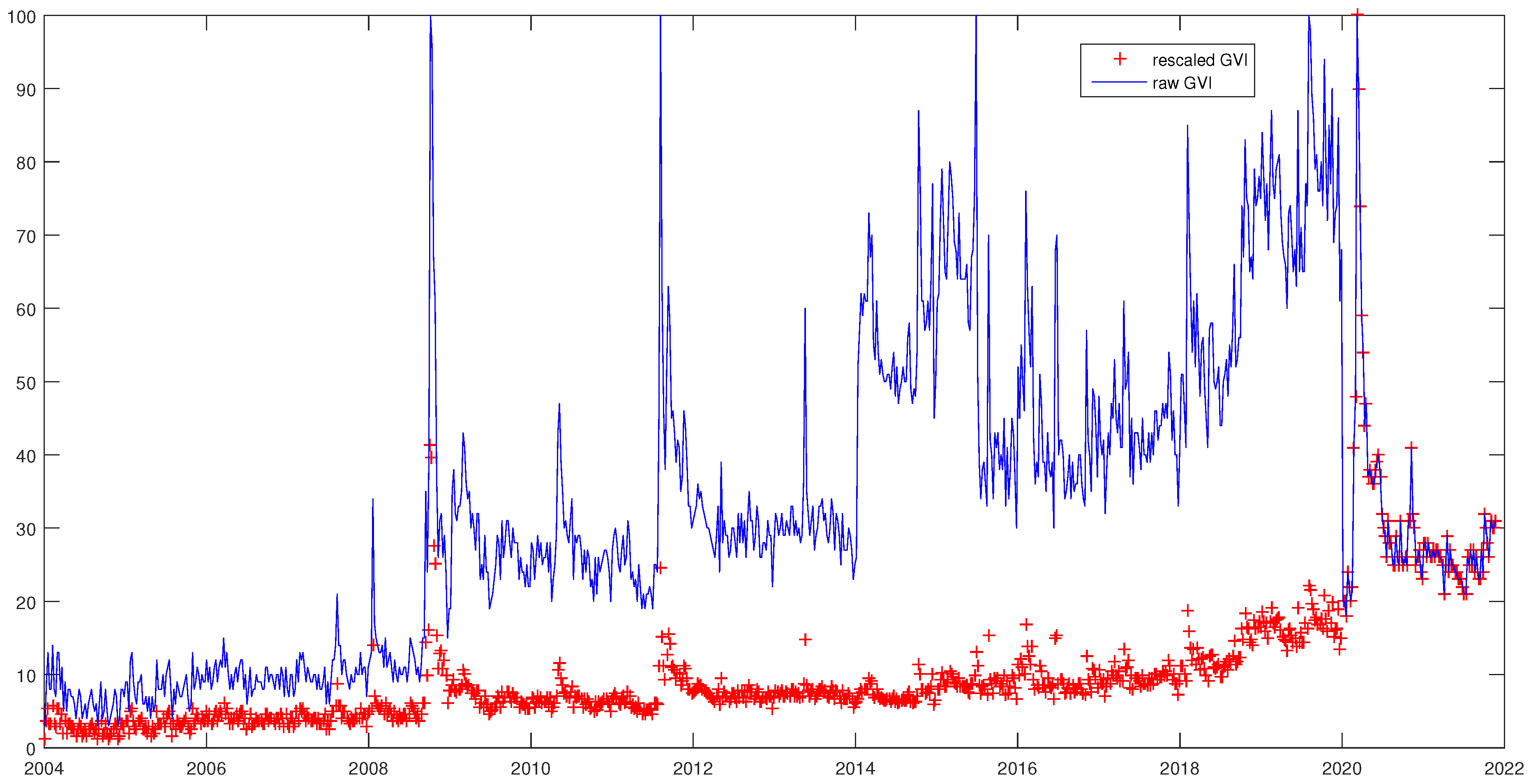
Appendix A. Rescaling Google Data

Let V t , t = 1 , , T , be the search volume of a specified query (for example “cac”) up to time T. The GVI at time t is given by:
G V I t = V t S · H · 100 , t = 1 , , T
where S is total search volume for query “cac” and H is the highest search volume for this query over period T defined by:
H = max V t S · H , t = 1 , , T
To merge two windows of observations, we proceeded as follows:
  • Step 1: We downloaded Google search data for query “cac” over period T 1 . We obtain the first sample E 1 : V 1 S 1 · H 1 · 100 , . , V T 1 S 1 · H 1 · 100 . Then we downloaded search data for the same search query over period T 2 , for T 2 = T 1 , , T 1 + n , and obtained the second sample E 2 : V T 1 S 2 · H 2 · 100 , . , V T 1 + n S 2 · H 2 · 100 . Note that these two samples may be of different size.
  • Step 2: We computed the sum of values, respectively, in samples E 1 and E 2 :
    K 1 = V 1 S 1 · H 1 · 100 + . + V T 1 S 1 · H 1 · 100 = t = 1 T 1 V t S 1 · H 1 · 100 = 1 H 1 · 100
    where t = 1 T 1 V t = S 1 . We then deduced:
    H 1 = 100 K 1
    We performed the same procedure for sample E 2 and deduced H 2 .
  • Step 3: We divided the last value in E 1 by the first value in E 2 :
    F = V T 1 S 1 · H 1 · 100 V T 1 S 2 · H 2 · 100 = S 2 · H 2 S 1 · H 1
    Then, we multiplied the resulting value F by H 1 H 2 :
    F · H 1 H 2 = S 2 · H 2 S 1 · H 1 · H 1 H 2 = S 2 S 1
    The resulting value S 2 S 1 will be used in next step.
  • Step 4: We determined the effective total search volume S over the period T = 1 , , T 1 + n (since the GVI at time T 1 is duplicated in the dataset):
    r = S 2 S 1 V T 1 S 1 = S 2 V T 1 S 1 = S 2 S 1 S 2 = S 1 · r
    As a result, the total search volume S is:
    S = S 1 + S 2 = ( 1 + r ) · S 1 = r · S 1
  • Step 5: We multiplied values in E 1 by H 1 100 and divided by r . We then obtained V 1 S 1 · r , , V T 1 S 1 · r . Then, we multiplied G V I t values, t = T 1 + 1 , , T 1 + n , in E 2 by ( S 2 S 1 · H 2 · 100 ) and divided by r . As a result, we obtained V T 1 + 1 S 1 · r , , V T 1 + n S 1 · r . Then, we merged these samples into one sample E: V 1 S 1 · r , , V T 1 + n S 1 · r .
  • Step 6: We determined the highest relative search volume in E as:
    H = max V t S 1 · r , t = 1 , , T 1 + n
  • Step 7: We divided each value in E by H and multiply by 100 to obtain the rescaled data: V 1 S 1 · r · H · 100 , , V T 1 + n S 1 · r · H · 100 .
In Figure A1, we plot raw GVI data (we merged windows without rescaling) and rescaled data using our method for the search query “cac”. Note that our method allows us to use normalized data (without scaling): V 1 S 1 · r , , V T 1 + n S 1 · r . However, in our study we use normalized and scaled GVI data in order to compare our results with those reported in previous studies.
Figure A1. Raw and rescaled GVI for query “cac”.
Jrfm 15 00066 g0a1

Notes

1
According to NetMarketShare (https://netmarketshare.com, accessed on 3 November 2021), Google holds 72.38 % of the market share in 2020.
2
The data are publicly available from http://www.google.com/trends, accessed on 28 November 2021.
3
https://gs.statcounter.com, accessed on 3 November 2021.

References

  1. Andersen, Torben G., Tim Bollerslev, and Francis X. Diebold. 2007. Roughing it up: Including jump components in the measurement, modeling, and forecasting of return volatility. The Review of Economics and Statistics 89: 701–20. [Google Scholar] [CrossRef]
  2. Andrei, Daniel, and Michael Hasler. 2014. Investor attention and stock market volatility. The Review of Financial Studies 28: 33–72. [Google Scholar] [CrossRef]
  3. Bank, Matthias, Martin Larch, and Georg Peter. 2011. Google search volume and its influence on liquidity and returns of german stocks. Financial Markets and Portfolio Management 25: 239. [Google Scholar] [CrossRef]
  4. Barber, Brad M., and Terrance Odean. 2008. All that glitters: The effect of attention and news on the buying behavior of individual and institutional investors. The Review of Financial Studies 21: 785–818. [Google Scholar] [CrossRef] [Green Version]
  5. Bollerslev, Tim, Hood Benjamin, Huss John, and Lasse H. Pedersen. 2018. Risk Everywhere: Modeling and Managing Volatility. The Review of Financial Studies 31: 2729–73. [Google Scholar] [CrossRef]
  6. Carneiro, Herman Anthony, and Eleftherios Mylonakis. 2009. Google trends: A web-based tool for real-time surveillance of disease outbreaks. Clinical Infectious Diseases 49: 1557–64. [Google Scholar] [CrossRef]
  7. Chen, Tao. 2017. Investor attention and global stock returns. Journal of Behavioral Finance 18: 358–72. [Google Scholar] [CrossRef]
  8. Choi, Hyunyoung, and Hal Varian. 2012. Predicting the present with google trends. Economic Record 88: 2–9. [Google Scholar] [CrossRef]
  9. Corsi, Fulvio. 2009. A simple approximate long-memory model of realized volatility. Journal of Financial Econometrics 7: 174–96. [Google Scholar] [CrossRef]
  10. Corsi, Fulvio, and Roberto Renò. 2012. Discrete-time volatility forecasting with persistent leverage effect and the link with continuous-time volatility modeling. Journal of Business & Economic Statistics 30: 368–80. [Google Scholar]
  11. Da, Zhi, Joseph Engelberg, and Pengjie Gao. 2011. In search of attention. The Journal of Finance 66: 1461–99. [Google Scholar] [CrossRef]
  12. Dellavigna, Stefano, and Joshua M. Pollet. 2009. Investor inattention and friday earnings announcements. The Journal of Finance 64: 709–49. [Google Scholar] [CrossRef] [Green Version]
  13. Diebold, Francis X., and Roberto S. Mariano. 1995. Comparing predictive accuracy. Journal of Business & Economic Statistics 13: 253–63. [Google Scholar]
  14. Dimpfl, Thomas, and Stephan Jank. 2016. Can internet search queries help to predict stock market volatility? European Financial Management 22: 171–92. [Google Scholar] [CrossRef] [Green Version]
  15. Ekinci, Cumhur, and Ali Eray Bulut. 2021. Google search and stock returns: A study on bist 100 stocks. Global Finance Journal 47: 100518. [Google Scholar] [CrossRef]
  16. Ginsberg, Jeremy, Matthew H. Mohebbi, Rajan S. Patel, Lynnette Brammer, Mark S. Smolinski, and Larry Brilliant. 2009. Detecting influenza epidemics using search engine query data. Nature 457: 1012–14. [Google Scholar] [CrossRef]
  17. Golosnoy, Vasyl, Alain Hamid, and Yarema Okhrin. 2014. The empirical similarity approach for volatility prediction. Journal of Banking & Finance 40: 321–29. [Google Scholar]
  18. Grullon, Gustavo, Kanatas George, and James P. Weston. 2004. Advertising, breadth of ownership, and liquidity. Review of Financial Studies 17: 439–61. [Google Scholar] [CrossRef]
  19. Guzman, Giselle. 2011. Internet search behavior as an economic forecasting tool: The case of inflation expectations. Journal of Economic and Social Measurement 36: 119–67. [Google Scholar] [CrossRef]
  20. Hamid, Alain. 2015. Prediction power of high-frequency based volatility measures: A model based approach. Review of Managerial Science 9: 549–76. [Google Scholar] [CrossRef]
  21. Hamid, Alain, and Moritz Heiden. 2015. Forecasting volatility with empirical similarity and google trends. Journal of Economic Behavior & Organization 117: 62–81. [Google Scholar]
  22. Hansen, Peter R., Asger Lunde, and James M. Nason. 2011. The model confidence set. Econometrica 79: 453–97. [Google Scholar] [CrossRef] [Green Version]
  23. Hasler, Michael, and Chayawat Ornthanalai. 2018. Fluctuating attention and financial contagion. Journal of Monetary Economics 99: 106–23. [Google Scholar] [CrossRef]
  24. Heber, Gerd, Asger Lunde, Neil Shephard, and Kevin Sheppard. 2009. Oxford-Man Institute’s Realized Library, Version 0.1. Available online: https://realized.oxford-man.ox.ac.uk/ (accessed on 3 November 2021).
  25. Hirshleifer, David, Sonya Seongyeon Lim, and Siew Hong Teoh. 2009. Driven to distraction: Extraneous events and underreaction to earnings news. The Journal of Finance 64: 2289–325. [Google Scholar] [CrossRef] [Green Version]
  26. Hou, Kewei, Wei Xiong, and Lin Peng. 2009. A Tale of Two Anomalies: The Implications of Investor Attention for Price and Earnings Momentum. Working Paper. Available online: https://ssrn.com/abstract=976394 (accessed on 3 November 2021).
  27. Joseph, Kissan, M. Babajide Wintoki, and Zelin Zhang. 2011. Forecasting abnormal stock returns and trading volume using investor sentiment: Evidence from online search. International Journal of Forecasting 27: 1116–27. [Google Scholar] [CrossRef]
  28. Kahneman, Daniel. 1973. Attention and Effort. Englewood Cliffs: Prentice-Hall, vol. 1063. [Google Scholar]
  29. Kim, Neri, Katarína Lučivjanská, Peter Molnár, and Roviel Villa. 2019. Google searches and stock market activity: Evidence from norway. Finance Research Letters 28: 208–20. [Google Scholar] [CrossRef]
  30. Klemola, Antti, Jussi Nikkinen, and Jarkko Peltomäki. 2016. Changes in investors’ market attention and near-term stock market returns. Journal of Behavioral Finance 17: 18–30. [Google Scholar] [CrossRef]
  31. Lieberman, Offer. 2012. A similarity-based approach to time-varying coefficient non-stationary autoregression. Journal of Time Series Analysis 33: 484–502. [Google Scholar] [CrossRef]
  32. Liu, Lily Y., Andrew J. Patton, and Kevin Sheppard. 2015. Does anything beat 5-minute rv? A comparison of realized measures across multiple asset classes. Journal of Econometrics 187: 293–311. [Google Scholar] [CrossRef] [Green Version]
  33. Mondria, Jordi, and Climent Quintana-Domeque. 2013. Financial contagion and attention allocation. The Economic Journal 123: 429–54. [Google Scholar] [CrossRef] [Green Version]
  34. Padungsaksawasdi, Chaiyuth, Sirim on Treepongkaruna, and Robert Brooks. 2019. Investor attention and stock market activities: New evidence from panel data. International Journal of Financial Studies 7: 30. [Google Scholar] [CrossRef] [Green Version]
  35. Patton, Andrew J. 2011. Volatility forecast comparison using imperfect volatility proxies. Journal of Econometrics 160: 246–56. [Google Scholar] [CrossRef] [Green Version]
  36. Patton, Andrew J., and Kevin Sheppard. 2009. Evaluating volatility and correlation forecasts. In Handbook of Financial Time Series. Berlin/Heidelberg: Springer, pp. 801–38. [Google Scholar]
  37. Peng, Lin, and Wei Xiong. 2006. Investor attention, overconfidence and category learning. Journal of Financial Economics 80: 563–602. [Google Scholar] [CrossRef] [Green Version]
  38. Politis, Dimitris N., and Joseph P. Romano. 1994. The stationary bootstrap. Journal of the American Statistical Association 89: 1303–13. [Google Scholar] [CrossRef]
  39. Seasholes, Mark S., and Guojun Wu. 2007. Predictable behavior, profits, and attention. Journal of Empirical Finance 14: 590–610. [Google Scholar] [CrossRef]
  40. Simon, Herbert A. 1955. A behavioral model of rational choice. The Quarterly Journal of Economics 69: 99–118. [Google Scholar] [CrossRef]
  41. Vlastakis, Nikolaos, and Raphael N. Markellos. 2012. Information demand and stock market volatility. Journal of Banking & Finance 36: 1808–21. [Google Scholar]
  42. Vosen, Simeon, and Torsten Schmidt. 2011. Forecasting private consumption: Survey-based indicators vs. google trends. Journal of Forecasting 30: 565–78. [Google Scholar] [CrossRef] [Green Version]
  43. Vozlyublennaia, Nadia. 2014. Investor attention, index performance, and return predictability. Journal of Banking & Finance 41: 17–35. [Google Scholar]
  44. Wang, Hua, Liao Xu, and Susan Sunila Sharma. 2021. Does investor attention increase stock market volatility during the COVID-19 pandemic? Pacific-Basin Finance Journal 69: 101638. [Google Scholar] [CrossRef]
  45. Wen, Fenghua, Longhao Xu, Guangda Ouyang, and Gang Kou. 2019. Retail investor attention and stock price crash risk: Evidence from china. International Review of Financial Analysis 65: 101376. [Google Scholar]
  46. Yang, Xin, Bing Pan, James A. Evans, and Benfu Lv. 2015. Forecasting chinese tourist volume with search engine data. Tourism Management 46: 386–97. [Google Scholar] [CrossRef]
Figure 1. Weekly RV and GVI. For comparability, the GVI data were scaled by 10 4 .
Jrfm 15 00066 g001aJrfm 15 00066 g001b
Figure 2. Time plot of coefficient estimates β t (beta) and the autoregressive coefficient (ar1), respectively, for the ES and AR(1) models (top) for DJIA (left) and Bovespa (right). Time-series of realized volatility and the corresponding GVI data (bottom) for DJIA (left) and Bovespa (right).
Jrfm 15 00066 g002
Figure 3. Time-varying empirical similarity (phi1, phi2 and phi3) under the HAR-ES model and HAR coefficient estimates (har1, har2 and har3) for the AEX index. Time-series of realized volatility and the corresponding GVI data are displayed in the bottom panel.
Jrfm 15 00066 g003
Table 1. List of stock market indices and search terms.
IndexCountrySearch Term
AEXNetherlands“aex”
All OrdinariesAustralia“all ordinaries”
BEL 20Belgium“bel 20”
BovespaBrazil“bovespa”
BSE SensexIndia“sensex”
CAC 40France“cac”
DAXGermany“dax”
DJIAU.S“dow”
FTSE 100U.K”ftse”
Hang SengChina“hang seng index”
IBEX 35Spain“ibex”
IPCMexico“ipc”
Nikkei 225Japan“nikkei 225”
SMISwitzerland“smi”
Table 2. Summary statistics for RV and GVI.
IndexRealized VolatilityGVICorr
MeanMinMaxSkewKurt ρ ( 1 ) ADF Mean Min Max Skew Kurt ρ ( 1 ) ADF
AEX4.69 × 10 4 1.43 × 10 5 1.13 × 10 2 7.0767.690.803.35 × 10 22 1.18 × 10 3 2.38 × 10 4 1.00 × 10 2 4.7440.450.888.68 × 10 12 0.66
All Ordinaries2.78 × 10 4 6.25 × 10 6 9.10 × 10 3 10.43140.250.794.38 × 10 17 1.43 × 10 3 0.00 × 10 0 1.00 × 10 2 1.958.610.677.87 × 10 5 0.50
BEL 204.05 × 10 4 3.38 × 10 5 9.63 × 10 3 7.3575.340.763.74 × 10 23 1.31 × 10 3 0.00 × 10 0 1.00 × 10 2 2.4512.140.932.32 × 10 3 0.47
Bovespa7.24 × 10 4 5.62 × 10 5 1.55 × 10 2 7.2367.870.802.46 × 10 10 1.77 × 10 3 4.68 × 10 4 1.00 × 10 2 2.3412.960.902.44 × 10 5 0.61
BSE Sensex6.25 × 10 4 1.87 × 10 5 1.96 × 10 2 8.67102.660.478.42 × 10 28 2.14 × 10 3 0.00 × 10 0 1.00 × 10 2 1.394.990.891.45 × 10 3 0.34
CAC 405.61 × 10 4 3.98 × 10 5 1.31 × 10 2 7.2172.500.757.52 × 10 12 1.02 × 10 3 1.24 × 10 4 1.00 × 10 2 3.5324.430.945.75 × 10 5 0.44
DAX5.76 × 10 4 1.41 × 10 5 1.34 × 10 2 7.1770.790.711.83 × 10 11 7.82 × 10 4 1.28 × 10 4 1.00 × 10 2 4.7438.820.941.75 × 10 4 0.29
DJIA4.95 × 10 4 1.70 × 10 5 1.50 × 10 2 7.5270.420.777.27 × 10 11 7.95 × 10 4 1.93 × 10 4 1.00 × 10 2 4.4936.960.932.46 × 10 7 0.47
FTSE 1005.50 × 10 4 2.75 × 10 5 1.88 × 10 2 8.86108.170.686.69 × 10 17 1.11 × 10 3 1.25 × 10 4 1.00 × 10 2 2.5511.430.951.00 × 10 4 0.27
Hang Seng4.17 × 10 4 2.76 × 10 5 1.35 × 10 2 9.81153.490.682.95 × 10 7 1.36 × 10 3 0.00 × 10 0 1.00 × 10 2 2.087.200.955.78 × 10 1 0.11
IBEX 356.55 × 10 4 3.05 × 10 5 9.59 × 10 3 5.1238.690.713.58 × 10 26 1.86 × 10 3 1.41 × 10 4 1.00 × 10 2 1.254.820.965.99 × 10 1 0.16
IPC3.95 × 10 4 3.10 × 10 5 8.45 × 10 3 7.5279.830.655.08 × 10 12 1.45 × 10 3 0.00 × 10 0 1.00 × 10 2 2.4316.110.411.49 × 10 5 0.18
Nikkei 2254.23 × 10 4 2.09 × 10 5 1.07 × 10 2 7.1374.790.652.58 × 10 16 2.09 × 10 3 3.00 × 10 4 1.00 × 10 2 1.8710.970.731.02 × 10 10 0.50
SMI3.69 × 10 4 2.27 × 10 5 1.32 × 10 2 9.78127.280.738.91 × 10 26 6.65 × 10 4 0.00 × 10 0 1.00 × 10 2 4.5235.090.931.05 × 10 2 0.49
This table reports summary statistics for realized volatility and GVI series for our sample indices. We report the mean, minimum (min), maximum (max), skewness (skew), kurtosis (kurt), the autocorrelation coefficient of the first order ρ(1), the p-value of the ADF test and the correlation coefficient between RV and GVI (Corr). For comparability, GVI data were scaled by 10−4.
Table 3. Linear Granger causality test.
Index H 0 : GVI Does Not Granger Cause RV H 0 : RV Does Not Granger Cause GVIResults
F-Statisticyyp-ValueF-Statisticp-Value
AEX22.3710.0008.2580.000 G R V
All ordinaries3.5390.0074.1630.002 G R V
BEL 2014.2530.00013.2980.000 G R V
Bovespa17.3240.00017.5490.000 G R V
BSE Sensex3.5330.0078.8090.000 G R V
CAC 4029.3490.00013.3690.000 G R V
DAX23.1010.00012.4660.000 G R V
DJIA14.7540.0008.9940.000 G R V
FTSE 1002.0470.08612.9310.000 G R V
Hang Seng0.4340.7844.3660.002 R V G
IBEX 351.4390.2199.9910.000 R V G
IPC1.2180.3021.1630.326 X
NIKKEI 2254.3500.0024.9880.001 G R V
SMI22.9910.00010.8260.000 G R V
This table reports the F-statistics (Wald statistics) and the p-values of the Granger causality test. “→” denotes unidirectional causality, “↔” denotes bidirectional causality and “X” means no Granger causality.
Table 4. VAR estimation results.
AEXAll OrdinariesBEL 20BovespaBSE SensexCAC 40DAX
RV t G t RV t G t RV t G t RV t G t RV t G t RV t G t RV t G t
C o n s t . × 10 4 1.039 c 1.063 c 0.183 2.606 c 0.806 c 0.687 c 0.086 0.758 b 2.228 c 1.455 c 1.296 c 0.652 c 1.348 c 0.582 c
(0.001)(0.000)(0.345)(0.000)(0.000)(0.001)(0.856)(0.014)(0.001)(0.000)(0.000)(0.000)(0.000)(0.000)
R V t 1 0.560 c 0.026 0.815 c 0.328 c 0.713 c 0.175 c 0.557 c 0.091 c 0.325 c 0.040 a 0.469 c −0.015 0.403 c 0.059 c
(0.000)(0.465)(0.000)(0.000)(0.000)(0.000)(0.000)(0.000)(0.000)(0.077)(0.000)(0.472)(0.000)(0.000)
R V t 2 −0.083 0.149 c 0.155 c 0.272 c 0.163 c 0.186 c −0.004 0.165 c 0.109 b 0.033−0.058 0.097 c 0.162 c 0.047 c
(0.137)(0.000)(0.000)(0.007)(0.000)(0.000)(0.927)(0.000)(0.012)(0.172)(0.221)(0.000)(0.000)(0.005)
R V t 3 0.148 c −0.003 0.422 c 0.0040.07−0.005 0.242 c −0.0190.048 0.053 b 0.293 c 0.046 b 0.425 c 0.070 c
(0.006)(0.944)(0.000)(0.970)(0.115)(0.913)(0.000)(0.515)(0.268)(0.029)(0.000)(0.035)(0.000)(0.000)
R V t 4 0.169 c 0.030 0.183 c 0.002 0.111 c 0.086 b −0.009−0.016 0.123 c −0.0010.069−0.011 0.196 c −0.009
(0.000)(0.390)(0.000)(0.985)(0.002)(0.015)(0.829)(0.525)(0.003)(0.961)(0.105)(0.586)(0.000)(0.557)
G t 1 0.597 c 0.807 c 0.037 c 0.385 c 0.216 c 0.526 c 0.435 c 0.590 c 0.140 a 0.573 c 0.969 c 0.926 c 0.856 c 1.084 c
(0.000)(0.000)(0.009)(0.000)(0.000)(0.000)(0.000)(0.000)(0.060)(0.000)(0.000)(0.000)(0.000)(0.000)
G t 2 −0.095 0.248 c −0.002 0.231 c 0.098 b 0.381 c 0.037 0.193 c 0.053 0.200 c 0.338 c 0.182 c 0.638 c 0.112 b
(0.216)(0.000)(0.913)(0.000)(0.022)(0.000)(0.586)(0.000)(0.524)(0.000)(0.003)(0.001)(0.000)(0.030)
G t 3 0.322 c 0.110 b 0.015 0.111 c 0.154 c −0.005 0.169 b 0.125 c 0.072 0.163 c 0.450 c 0.143 c 0.523 c 0.425 c
(0.000)(0.049)(0.322)(0.003)(0.000)(0.903)(0.012)(0.004)(0.390)(0.000)(0.000)(0.008)(0.00)0(0.000)
G t 4 0.186 c 0.005−0.01 0.085 b 0.141 c 0.081 b 0.221 c 0.093 b 0.257 c 0.037 0.188 a 0.017 0.284 c 0.191 c
(0.008)(0.929)(0.480)(0.013)(0.000)(0.034)(0.000)(0.023)(0.001)(0.373)(0.053)(0.715)(0.003)(0.000)
Adj. R 2 0.6710.7850.6660.5280.6110.8860.6640.8260.2560.8310.6180.9030.5870.906
DJIAFTSE 100Hang SengIBEX 35IPCNikkei 225SMI
RV t G t RV t G t RV t G t RV t G t RV t G t RV t G t RV t G t
C o n s t . × 10 4 1.159 c 0.620 a 1.635 c 0.576 c 0.913 c 0.704 c 2.022 c 0.788 c 1.096 c 4.455 c 0.800 a 3.412 c 1.079 c 0.494 c
(0.001)(0.100)(0.000)(0.001)(0.000)(0.001)(0.000)(0.000)(0.002)(0.000)(0.061)(0.000)(0.000)(0.000)
R V t 1 0.590 c 0.032 a 0.611 c 0.083 c 0.480 c 0.039 0.689 c 0.065 c 0.546 c 0.046 0.474 c 0.048 0.528 c 0.035
(0.000)(0.100)(0.000)(0.000)(0.000)(0.243)(0.000)(0.002)(0.000)(0.440)(0.000)(0.344)(0.000)(0.157)
R V t 2 0.111 b 0.069 c −0.043 0.102 c 0.119 c 0.085 b 0.100 b 0.095 c 0.086 b 0.071 0.189 c 0.026 0.113 b 0.079 c
(0.033)(0.002)(0.316)(0.000)(0.002)(0.017)(0.031)(0.000)(0.022)(0.292)(0.000)(0.721)(0.023)(0.004)
R V t 3 0.297 c 0.045 b 0.170 c 0.009 0.234 c 0.008 0.083 a 0.004 0.092 b −0.029 0.136 c −0.008 0.165 c 0.012
(0.000)(0.046)(0.000)(0.647)(0.000)(0.819)(0.074)(0.877)(0.015)(0.663)(0.001)(0.892)(0.001)(0.663)
R V t 4 0.0280.005−0.003 0.034 b −0.038−0.05 0.068 a 0.041 a −0.003−0.084 0.076 b 0.191 c 0.118 c 0.063 c
(0.535)(0.802)(0.932)(0.045)(0.292)(0.135)(0.083)(0.054)(0.931)(0.158)(0.043)(0.000)(0.006)(0.008)
G t 1 0.538 c 0.960 c 0.079 0.800 c 0.022 0.558 c 0.093 0.682 c 0.0198 0.241 c 0.022 0.503 c 0.696 c 0.842 c
(0.000)(0.000)(0.361)(0.000)(0.562)(0.000)(0.201)(0.000)(0.283)(0.000)(0.421)(0.000)(0.000)(0.000)
G t 2 0.107 0.134 b 0.1400.0780.005 0.263 c 0.038 0.157 c 0.007 0.160 c 0.007 0.087 b −0.109 0.137 c
(0.419)(0.020)(0.201)(0.110)(0.900)(0.000)(0.663)(0.001)(0.720)(0.000)(0.809)(0.038)(0.255)(0.010)
G t 3 0.532 c 0.159 c 0.251 b 0.009−0.053 0.076 a −0.047 0.091 a 0.011 0.146 c 0.089 c 0.177 c 0.413 c 0.095 a
(0.000)(0.006)(0.021)(0.846)(0.228)(0.062)(0.589)(0.054)(0.542)(0.000)(0.004)(0.000)(0.000)(0.073)
G t 4 −0.1390.0210.016 0.087 b 0.02 0.085 b −0.1010.056 0.037 b 0.142 c 0.102 c 0.098 c 0.173 b 0.100 b
(0.185)(0.645)(0.845)(0.018)(0.599)(0.017)(0.165)(0.152)(0.042)(0.000)(0.000)(0.010)(0.036)(0.030)
Adj. R 2 0.6270.8620.4750.9100.5040.9200.5050.9410.4360.2650.4820.5700.5830.884
This table reports VAR estimation results for our sample indices. The first column reports the estimated coefficients with realized volatility as the dependent variable. The second column reports the estimated coefficients with Google Volume Index (denoted simply by G) as the dependent variable. Coefficient estimates are followed by p-values in parentheses. Superscripts a, b and c denote statistical significance, respectively, at the 10%, 5% and 1% levels.
Table 5. In-sample results of predictive regressions.
IndexARAR-GESHARHAR-GHAR-ES
w 0 × 10 3 w 1 w 0 × 10 3 w 1 g 1 w 0 × 10 3 w 1 w 0 × 10 3 w 1 w 2 w 3 w 0 × 10 3 w 1 w 2 w 3 g 1 w 1 w 2 w 3
AEX 0.096 c 0.795 c 0.034 0.754 c 0.069 b −0.012 142.997 c 0.070 c 0.821 c 0.105 b 0.135 c −0.003 0.777 c 0.115 c 0.146 c 0.079 c 1269.054 c 287.970 c 675.690 c
(0.000)(0.000)(0.295)(0.000)(0.017)(0.457)(0.000)(0.003)(0.000)(0.017)(0.003)(0.924)(0.000)(0.009)(0.001)(0.007)(0.000)(0.002)(0.001)
All Ordinaries 0.059 c 0.789 c 0.009 0.744 c 0.043 c −0.015 41.545 c 0.054 c 0.849 c 0.134 c 0.093 b 0.009 0.809 c 0.136 c 0.044 0.050 c 1546.964 c 569.113 c −984.755
(0.000)(0.000)(0.607)(0.000)(0.000)(0.240)(0.000)(0.001)(0.000)( 0.002)(0.047)(0.636)(0.000)(0.001)(0.358)(0.000)(0.000)(0.000)(0.234)
BEL 20 0.095 c 0.765 c 0.059 c 0.734 c 0.037 c −0.018 57.915 c 0.067 c 0.774 c 0.083 a 0.146 c 0.039 a 0.756 c 0.093 b 0.130 c 0.034 b 42,339.7592774.897−4383.604
(0.000)(0.000)(0.005)(0.000)(0.005)(0.208)(0.000)(0.001)(0.000)(0.072)(0.003)(0.096)(0.000)(0.045)(0.009)(0.013)(0.119)(0.101)(0.167)
Bovespa 0.147 c 0.796 c −0.049 0.718 c 0.143 c −0.013 63.347 c 0.124 c 0.734 c 0.093 b −0.001−0.061 0.655 c 0.105 b −0.033 0.144 c 1273.227 c 164.609 c 420.271 c
(0.000)(0.000)(0.292)(0.000)(0.000)(0.571)(0.000)(0.000)(0.000)(0.043)(0.986)(0.219)(0.000)(0.020)(0.426)(0.000)(0.000)(0.000)(0.000)
BSE Sensex 0.329 c 0.472 c 0.268 c 0.460 c 0.032−0.046 124.669 c 0.137 c 0.454 c 0.155 c 0.148 b 0.110 a 0.446 c 0.156 c 0.146 b 0.015 446.008 c −92.085 460.747 b
(0.000)(0.000)(0.000)(0.000)(0.227)(0.179)(0.000)(0.001)(0.000)(0.005)(0.019)(0.059)(0.000)(0.005)(0.022)(0.499)(0.000)(0.295)(0.033)
CAC 40 0.140 c 0.751 c 0.099 c 0.730 c 0.051 b 0.016 81.712 c 0.094 c 0.713 c 0.009 0.112 b 0.053 0.695 c 0.001 0.117 b 0.051 a 42.540 171.112 c 286.492 c
(0.000)(0.000)(0.002)(0.000)(0.050)(0.417)(0.000)(0.002)(0.000)(0.853)(0.025)(0.151)(0.000)(0.977)(0.019)(0.053)(0.222)(0.003)(0.006)
DAX 0.168 c 0.709 c 0.157 c 0.704 c 0.0170.027 54.473 c 0.099 c 0.567 c 0.185 c 0.075 0.083 b 0.561 c 0.183 c 0.0790.02422.988 111.911 b 124.812 b
(0.000)(0.000)(0.000)(0.000)(0.549)(0.227)(0.000)(0.002)(0.000)(0.001)(0.149)(0.029)(0.000)(0.001)(0.129)(0.405)(0.379)(0.012)(0.019)
DJIA 0.112 c 0.775 c 0.091 c 0.764 c 0.0320.023 34.596 c 0.084 c 0.717 c 0.066 b 0.049 0.064 a 0.707 c 0.0660.0490.030 109.116 c −52.484 103.537 b
(0.000)(0.000)(0.007)(0.000)(0.328)(0.342)(0.000)(0.006)(0.000)(0.160)(0.286)(0.082)(0.000)(0.161)(0.290)(0.364)(0.000)(0.206)(0.021)
FTSE 100 0.176 c 0.682 c 0.176 c 0.682 c −0.0010.019 40.070 c 0.111 c 0.598 c 0.091 a 0.113 b 0.117 c 0.600 c 0.092 a 0.113 b −0.006 37.084 c 49.035−68.857
(0.000)(0.000)(0.000)(0.000)(0.965)(0.479)(0.000)(0.003)(0.000)(0.088)(0.046)(0.007)(0.000)(0.086)(0.046)(0.793)(0.005)(0.379)(0.192)
Hang Seng 0.134 c 0.677 c 0.141 c 0.679 c −0.006−0.006 50.628 c 0.065 c 0.445 c 0.311 c 0.085 0.067 b 0.445 c 0.311 c 0.085−0.001−380.84710,744.545 b 9748.689 b
(0.000)(0.000)(0.000)(0.000)(0.588)(0.684)(0.000)(0.003)(0.000)(0.000)(0.108)(0.012)(0.000)(0.000)(0.111)(0.931)(0.123)(0.046)(0.047)
IBEX 35 0.192 c 0.708 c 0.212 c 0.711 c −0.012−0.018 66.151 c 0.124 c 0.654 c 0.032 0.129 b 0.144 c 0.656 c 0.033 0.126 b −0.01122.545 165.073 a 154.976 b
(0.000)(0.000)(0.000)(0.000)(0.434)(0.386)(0.000)(0.000)(0.000)(0.539)(0.019)(0.001)(0.000)(0.527)(0.022)(0.481)(0.620)(0.092)(0.021)
IPC 0.138 c 0.651 c 0.119 c 0.647 c 0.015−0.013 71.642 c 0.085 c 0.515 c 0.201 c 0.070 0.059 a 0.510 c 0.197 c 0.0770.019 1274.233 c 14,116.551 c 2415.009 b
(0.000)(0.000)(0.000)(0.000)(0.358)(0.395)(0.000)(0.000)(0.000)(0.000)(0.231)(0.075)(0.000)(0.000)(0.193)(0.269)(0.003)(0.001)(0.016)
Nikkei 225 0.147 c 0.652 c 0.099 b 0.632 c 0.027−0.023 38.068 c 0.089 c 0.509 c 0.207 c 0.0690.032 0.485 c 0.208 c 0.072 0.031 2206.406 c 879.275 c −626.898
(0.000)(0.000)(0.012)(0.000)(0.161)(0.262)(0.002)(0.001)(0.000)(0.000)(0.230)(0.466)(0.000)(0.000)(0.213)(0.108)(0.000)(0.001)(0.262)
SMI 0.098 c 0.734 c 0.078 c 0.712 c 0.042 a 0.017 102.112 c 0.080 c 0.760 c 0.092 b 0.117 b 0.063 b 0.744 0.098 b 0.109 b 0.042 a 1485.263 c 1034.711 c 912.327 c
(0.000)(0.000)(0.001)(0.000)(0.082)(0.353)(0.000)(0.001)(0.000)(0.050)(0.033)(0.019)(0.000)(0.036)(0.047)(0.090)(0.000)(0.000)(0.005)
This table reports the estimation results of the AR, AR-G, ES, HAR, HAR-G and HAR-ES models. Estimated coefficients are followed by p-values in parentheses. Superscripts a, b and c denote statistical significance, respectively, at the 10%, 5% and 1% levels.
Table 6. Out-of-sample average losses.
IndexMAEMSEQLIKE
ARAR-GESHARHAR-GHAR-ESARAR-GESHARHAR-GHAR-ESARAR-GESHARHAR-GHAR-ES
AEX1.1301.1581.0841.2961.2911.0001.4051.4111.1122.6382.2261.0001.2271.3292.0291.1062.0081.000
All Ordinaries1.1451.2671.2241.4121.4641.0001.6871.4501.6343.4572.4041.0001.0391.1641.2491.0281.4241.000
BEL 201.1121.2241.0621.4931.3441.0001.4421.4121.1775.3601.7491.0001.1931.3031.0981.1581.5381.000
Bovespa1.0361.0691.0351.3681.1241.0001.2781.2380.8574.0261.3491.0001.2781.2380.8574.0261.3491.000
BSE Sensex1.2991.4351.2201.3031.3661.0001.3021.3481.0991.7701.5051.0001.2104.8711.3961.2231.1841.000
CAC 401.1131.3141.1741.4461.4001.0001.3151.4041.6574.5381.6221.0001.1941.6431.4061.1184.6501.000
DAX1.1061.1981.1191.3541.2881.0001.2511.3161.3692.9901.4781.0001.1652.1461.0831.1333.1481.000
DJIA1.0811.2941.1151.1351.3571.0001.0461.1141.5781.2341.1811.0001.0881.3210.9981.1575.2941.000
FTSE 1001.0741.1431.0701.1901.3091.0001.0081.0651.0841.7681.8191.0001.1531.3951.0971.02315.8711.000
Hang Seng1.1041.1341.1611.1231.1501.0001.1891.2812.2871.1851.2711.0001.1541.1521.3561.0521.0811.000
IBEX 351.0511.0451.0691.2081.16801.0001.1121.1271.0682.1471.8311.0001.1611.6871.2621.1201.3271.000
IPC1.0421.0501.1501.0481.0561.0000.9450.9461.2050.9890.9941.0001.0741.1551.4811.0841.1141.000
Nikkei 2251.0961.1521.0251.0721.1621.0001.0971.1521.1211.1611.1961.0001.1091.3341.5561.17623.1271.000
SMI1.3171.4411.1812.0832.6771.0002.6662.2061.42512.20016.2641.0001.2451.7291.0711.2802.3801.000
This table reports weekly average values for MAE, MSE and QLIKE. Results are relative to HAR-ES losses.
Table 7. Diebold–Mariano test based on the QLIKE losses.
IndexHARARHARESESESESHAR-ESHAR-ESHAR-ESHAR-ESHAR-ES
vs.vs.vs.vs.vs.vs.vs.vs.vs.vs.vs.vs.
ARAR-GHAR-GARAR-GHARHAR-GARAR-GHARHAR-GES
AEX 2.787 b 1.799 a −1.4811.2901.1201.4820.024 4.166 c 5.761 c 3.245 c 1.659 a 1.656 a
All Ordinaries−0.308 2.479 b 3.521 c 2.045 b 1.035 2.345 b −1.223−0.501 2.256 b −0.461 3.554 c 2.612 b
BEL 20−0.823 3.083 c 2.825 c −1.555 3.314 c −0.943 3.142 c 4.141 c 6.218 c 3.495 c 4.029 c −1.644
Bovespa1.329 1.983 b 1.669 a 3.277 c 1.792 a −0.849 1.726 a 0.087 1.980 b −1.310 1.755 a 3.744 c
BSE Sensex0.102−1.0140.3171.569−0.9621.038 1.863 a 2.201 b −1.072−1.516 2.032 b 3.255 c
CAC 40 1.724 a 3.895 c 2.267 b 2.144 b −1.630 2.821 c 2.079 b 3.830 c 5.555 c 2.607 b 2.340 b 4.160 c
DAX−0.676−1.399 1.706 a −1.256−1.511−0.740 1.753 a 2.449 b −1.632 2.460 b 1.819 a −1.330
DJIA0.802 3.157 c −1.118−1.615 3.357 c −1.522−1.162−1.030 2.682 b 1.837 a −1.1580.024
FTSE 100 2.528 b −1.155−1.286−0.516−1.2740.861−1.280 1.781 a 1.767 a −0.452−1.289−1.365
Hang Seng 2.629 b 0.096−1.638 1.799 a 1.664 a 2.631 b 2.274 b 3.091 c 2.978 c −1.574 2.190 b 3.132 c
IBEX 35−0.913−1.323 2.812 c 0.836−1.0281.193−0.445 3.213 c 1.726 a 2.562 b 3.304 c 2.458 b
IPC0.344−1.624−1.3731.4221.1301.3851.282 1.798 a 2.535 b 2.386 b 2.640 b 1.677 a
Nikkei 2250.497 1.884 a −1.200 2.893 c 1.361 2.081 b −1.179 1.944 a 2.550 b −1.432−1.210 3.857 c
SMI0.602 2.874 c 3.617 c 2.790 b 3.725 c 2.356 b 4.118 c 5.601 c 4.177 c 5.449 c 4.568 c −1.016
This table reports the t-statistics of the Diebold–Mariano test based on the QLIKE losses. Superscripts a, b and c denote statistical significance, respectively, at the 10%, 5% and 1% levels.
Table 8. Model Confidence Set p-values.
IndexMAEMSEQLIKE
ARAR-GESHARHAR-GHAR-ESARAR-GESHARHAR-GHAR-ESARAR-GESHARHAR-GHAR-ES
AEX0.0650.0650.0650.0650.0651.0000.3460.3460.4370.3460.3461.0000.0070.0070.0070.0140.0071.000
All Ordinaries0.1000.0920.1000.1000.0921.0000.2730.2730.2730.2730.2731.0000.8020.1500.1500.8020.1351.000
BEL 200.0100.0010.0520.0010.0011.0000.2580.2580.3360.2230.2231.0000.0130.0000.0620.0620.0001.000
Bovespa0.2340.1760.3230.0360.0361.0000.4460.4461.0000.2370.2370.4461.0000.0730.0730.0730.0730.917
BSE Sensex0.0310.0160.0310.0310.0291.0000.3910.3820.4670.3820.3821.0000.2390.1630.1630.2390.2391.000
CAC 400.0120.0010.0120.0120.0011.0000.2230.2230.2230.1540.1541.0000.0230.0230.0230.0660.0231.000
DAX0.0070.0070.0870.0070.0071.0000.1900.1630.1900.1210.1211.0000.2570.2570.2570.2570.2571.000
DJIA0.0440.0030.0440.0440.0021.0000.5720.3320.0940.3060.0941.0000.6460.0341.0000.3510.0340.980
FTSE 1000.1090.0710.0730.0730.0631.0000.8660.3260.3260.3260.3261.0000.0670.0670.2830.6470.0671.000
Hang Seng0.0640.0640.0640.0640.0521.0000.2670.2670.2670.2670.2671.0000.0760.0890.0250.1840.1391.000
IBEX 350.3640.3640.1190.1190.1191.0000.7340.4460.7340.4460.4461.0000.0660.0260.0660.0660.0261.000
IPC0.3570.3570.0050.3460.2611.0001.0000.8290.1610.7760.5510.7760.1880.1880.1880.1880.1881.000
Nikkei 2250.0270.0130.3730.0860.0181.0000.3740.3740.3740.3740.3741.0000.1890.0980.0860.1890.0861.000
SMI0.0700.0700.0700.0700.0701.0000.3000.3000.3000.3000.3001.0000.0080.0080.3660.0080.0081.000
This table reports the Model Confidence (MCS) p-values. Bold numbers indicate that the model is included in the MCS at a 90% confidence level. The p-value of the last “surviving” model (i.e., best model) is 1.
Publisher’s Note: MDPI stays neutral with regard to jurisdictional claims in published maps and institutional affiliations.

