Article

A State-of-the-Art Fund Performance Index: Higher-Order Omega and Its Consistency with Almost Stochastic Dominance

1
College of Economics and Management, Nanjing University of Aeronautics and Astronautics, Nanjing 211106, China
2
School of Business and Management, Royal Holloway, University of London, Egham TW20 0EX, UK
3
Group of Researchers Applying Physics in Economy and Sociology (GRAPES), Beauvallon, Rue de la Belle Jardinière, 483, 0021 Sart Tilman, Angleur, B-4031 Liège, Belgium
*
Authors to whom correspondence should be addressed.
J. Risk Financial Manag. 2022, 15(10), 438; https://doi.org/10.3390/jrfm15100438
Submission received: 3 July 2022 / Revised: 13 September 2022 / Accepted: 22 September 2022 / Published: 28 September 2022
(This article belongs to the Section Mathematics and Finance)

Abstract

:
This paper provides a mathematical proof and theoretical analysis of the one-to-one consistency between higher-order Omega and Almost Stochastic Dominance rules when evaluating fund performance. The consistency between higher-order Omega and Almost Nth-degree Stochastic Dominance reinforces the effectiveness of applying the higher-order Omega function in fund performance measurement, as the Almost Stochastic Dominance rules are more likely to be observed in real life. This study also clarifies that the higher-order Omega decreases when threshold L increases. The ranking of funds based on higher-order Omega changes at different thresholds. Hence, it is critical to specify the L so that the consistency holds. Through evaluating the performance of eleven U.S. funds between 2010 and 2020, we demonstrate the applications of the Nth-order Omega in the concept of Almost Stochastic Dominance rules. Furthermore, the empirical results also show the superiority of the Nth-order Omega over the traditional fund performance measure, i.e., Sharpe ratio and the lower-order Omega. The ranking of fund performance based on higher-order Omega is consistent with Almost Stochastic Dominance rules.

1. Introduction

Academics and investors are still skeptical about the effectiveness of traditional fund performance measures. The performance indexes such as the Sharpe ratio and Treynor ratio (Sharpe 1966; Treynor 1965) work only if the evaluated funds follow a normal distribution and/or investors make an investment decision based on mean-variance decision making. Furthermore, it is well-documented that higher-order moments such as skewness and kurtosis also play an important role in investors’ preference decision making, but they are often neglected (Harvey and Siddique 2000; Guidolin and Timmermann 2008; Stutzer 2000). Keating and Shadwick (2002) first introduced the Omega function to measure fund performance to address the shortcomings of the traditional fund performance measures. The Omega function is defined as the probability-weighted ratio of potential gains over possible losses at a given level of expected return. It uses the complete information of assets and portfolio return distributions (Chan and Nadarajah 2019; Yang et al. 2021). van Dyk et al. (2014) reported that Omega ratio provides useful information to investors in addition to that provided by the Sharpe ratio alone. Hence, the Omega function could perform effectively even if the returns do not follow a normal distribution. Moreover, it is proved that the Omega function provides a consistent ranking as the First-order Stochastic Dominance (hereafter, FSD) (Benhamou et al. 2019). Bi et al. (2019) extend the Omega function to the Nth-order Omega based on the concept of Almost Acceptance Dominance (hereafter, AAD). The Nth-order Omega includes the Omega function as a special case when N equals 1. The Nth-order Omega not only retains the best properties of Omega, that no assumption of return distribution is required, but also takes higher moments into account.
Performance indexes including Sharpe ratio, Omega function, and higher-order Omega, are based on evaluation of the trade-off between return and risk (Heufer 2014). Another popular framework of fund performance evaluation consists of Stochastic Dominance, Almost Stochastic Dominance, and a series of dominance rules that provide a ranking based on two assets return distributions. According to the dominance rules, investors will choose one risky asset over the other according to the ranking order. However, it is well-known that the Sharpe ratio is not consistent with the FSD (Klar and Muller 2018). The investors could make an irrational decision, i.e., choose the investment with a smaller return by maximizing the Sharpe ratio. Therefore, it is important to examine if there is one-to-one consistency between the Omega type of measure and the (Almost) Stochastic Dominance rules. No conclusion has been drawn from existing literature. Some studies support the consistency between the Omega ratio and Stochastic Dominance. For example, Fong (2016) showed the consistency between the Omega ratio and Second-order Stochastic Dominance (thereafter, SSD) by using a simple deformation of Omega. Their results suggest that all loss-averse and risk-averse investors could adopt the Omega ratio to make the same investment decision which is also suggested by the SSD rule. Guo et al. (2017) find that the Omega ratio is consistent with SSD rules when the threshold of the Omega function is less than the average return of a higher-return portfolio. Their findings were applied to test the efficiency of the Hongkong estate market. Similar conclusions are drawn by Guo et al. (2018) that the Omega ratio criterion is consistent with the Stochastic Dominance. Their findings were supported by testing fund data. However, Klar and Muller (2018) claimed that there was a consistent relationship between Omega function and FSD, but no consistency with SSD. In addition, they also used expectiles (Bellini et al. 2016) to prove that the Omega index is consistent with fractional stochastic order (1 + γ), which was proposed by Muller et al. (2017). Balder and Schweizer (2017) clarified when Omega ratio was consistent with Second-order Stochastic Dominance and when it was not. They also pointed out that in order to avoid the consistency problem, any Omega ratio below one should be discarded like a negative Sharpe ratio. Caporin et al. (2018) critiqued that the Omega function has been used excessively and inappropriately. They claimed that the relationship between threshold and mean return would affect the effectiveness of the Omega index, that is, the smaller threshold accounts for less variations between the Omega and SSD rankings. However, most of the extant literature is restricted to lower-order Stochastic Dominance, i.e., FSD or SSD. Bi et al. (2019) extended Klar and Muller’s (2018) work to a higher-order framework and proved the one-to-one consistency between higher-order Omega and its corresponding higher-order Stochastic Dominance. However, there are very limited discussions on the consistency of higher-order Omega with Stochastic Dominance criteria since the development of higher-order Omega.
Why is it critical to prove a consistent relationship between higher-order Omega and the series rules of Stochastic Dominance? Stochastic Dominance suffers the well-known partial order problem, only employing partial information on the investor’s preferences such as risk aversion. With Omega types of measures, including higher-order Omega (Bi et al. 2019), Omega (Keating and Shadwick 2002) can generate a complete order through analytical calculations. If the consistency between the two is proved, it does not only imply the use of Stochastic Dominance among portfolios but also confirms the decision making based on higher-order Omega. However, Stochastic Dominance rarely could be observed in real life compared to Almost Stochastic Dominance (Tzeng et al. 2013). To address this limitation, we turn to the Almost Stochastic Dominance rule. There is always an Almost Stochastic Dominance relation existing between the two portfolios corresponding to the degree no matter what the value of N is (Tzeng et al. 2013). If there is consistency found between higher-order Omega and Almost Stochastic Dominance, then the application of higher-order Omega would become more feasible.
To our best knowledge, there is no research examining consistency between higher-order Omega and Almost Stochastic Dominance yet. This paper contributes to knowledge by exploring whether the higher-order Omega is consistent with Almost Stochastic Dominance. We also demonstrate the application of the higher-order Omega using U.S. fund data and provide empirical evidence to show the consistency between higher-order Omega and Almost Stochastic Dominance. The remainder of the paper is structured as follows. Section 2 describes the relevant theoretical foundations, including Stochastic Dominance theory, Almost Stochastic Dominance theory, and higher-order Omega’s theoretical foundation. Section 3 focuses on the conjecture and mathematical proof of the relationship between higher-order Omega and Almost Stochastic Dominance. In this section, we prove that the First-order Omega is consistent with Almost First Stochastic Dominance (thereafter, AFSD) when the threshold is in L 1 , L 2 . L 1 and L 2 are arithmetic expressions of the thresholds L of Nth-order Omega and statistical value of Nth-degree Almost Stochastic Dominance. Furthermore, we also find the consistency for higher-order when N is greater than 1 under certain conditions. Section 4 applies the results from Section 3 to evaluate the performance of real fund data based on the First-, Second-, and Third-order Omega index and the corresponding First-, Second-, and Third-order Almost Stochastic Dominance. Finally, conclusions are drawn, and we summarize that the consistency of higher-order Omega and Almost Nth-order Stochastic Dominance proves the superiority of this approach when evaluating and ranking more than two portfolios.

2. Definitions and Theories

Bi et al. (2019) proposed a higher-order Omega index, which is free of the utility function form or/and distribution assumptions. This index is rooted in the framework of acceptance dominance. Bi et al. (2019) provide a theoretical foundation by showing the consistency between Stochastic Dominance and higher-order Omega. In this section, we examine the consistency between higher-order Omega and Almost Stochastic Dominance. In the subsequent sub-section, we provide a detailed description of the relevant theories including Stochastic Dominance theory, Almost Stochastic Dominance theory, and describe the higher-order Omega.

2.1. (Almost) Stochastic Dominance

Assume variables X, Y, and their second-order integral are,
F Z 2 φ = φ F Z 1 t d t ,   F Z 1 φ = F Z φ = P Z < φ , Z = X , Y .
According to Levy (2015), First-order Stochastic Dominance (FSD) is defined as:
Definition 1.
FSD: X F S D Y if and only if
F X 1 φ F Y 1 φ   f o r   a n y   φ R ,   F X 1 b F Y 1 b .
FSD correlates with the case where the first derivative of the utility function is non-negative. Increasing utility means that the investor is always willing to have more wealth or return when all other things are equal. Regardless of investors’ risk attitude, i.e., risk-neutral, risk-loving, or risk-averse, FSD is the valid criterion as long as the utility function has a non-negative first derivative.
Similarly, assume the Nth-order integral of X, Y as follows,
F Z N φ = φ F Z N 1 t d t ,   Z = X , Y .
Thus, Nth-degree Stochastic Dominance (thereafter, NSD), N 2 , could be defined.
Definition 2.
NSD: X N S D Y if and only if
F X N φ F Y N φ   f o r   a n y   φ R ,   F X N b F Y N b ,   n = 1 , 2 , , N .
When N = 2, it is the definition of Second-order Stochastic Dominance (SSD). The SSD requires the second derivative of the utility function to be less than zero, that is, SSD is only effective for risk-averse investors. If the utility function’s second derivative is positive, Risk-seeker Stochastic Dominance (SRSD) is its effectiveness criterion (Bai et al. 2015; Levy 2015).
When N = 3, Third-order Stochastic Dominance (TSD) requires the third derivative of investors’ utility function to be positive, namely, risk prudential. The theory of NSD has strict ordering. In other words, a higher-order SD such as SSD and TSD will be found provided the FSD is established.
There is also a so-called pathological preference, based on which the utility function is limited to construct Almost Stochastic Dominance (ANSD). Adopting the interpretation of ANSD by Tzeng et al. (2013), define as follows,
U N ε N = u | 1 n + 1 u n x > 0 ,   n = 1 , 2 , , N ,   a n d 1 N + 1 u N i n f 1 N + 1 u N x 1 ε N 1 , x S ^ N F X , F Y = x x , x ¯ : F X N > F Y N , F X N F Y N = x x ¯ F X N F Y N d x .
Definition 3.
ε N A N S D : 0 < ε N < 0.5 ,   N 1 ,   X ε N A N S D Y , if and only if
S ^ N F X , F Y F X N x F Y N x d x ε N F X N F Y N , F Y n x ¯ F X n x ¯ 0 , n = 1 , 2 , , N .
Compared with Nth-degree Stochastic Dominance, Almost Nth-degree Stochastic Dominance eliminates unusual pathological preferences. It can be also seen from the mathematical expression as the critical condition to satisfy Stochastic Dominance. The condition specifies that one cumulative distribution is ‘absolutely greater’ than another for all distributions, while Almost Stochastic Dominance only requires ‘the relatively greater’ as a whole distribution. This also explains why the Almost Stochastic Dominance relationship is always found between any two portfolios, but not the Stochastic Dominance. This motivates us to prove the consistency between higher-order Omega and Almost Stochastic Dominance.

2.2. Higher-Order Omega

Similarly, consider a random variable x a , b ,   where   a < 0 < b , cumulative distribution function (CDF) and Nth-order integral of x is defined as:
F 1 x = F x = P X x ,   x a , b , F N x = a x F N 1 t d t .
Let O be a CDF of threshold L, similarly defined,
O N x = a x O N 1 t d t ,   a n d   O x = 0 , x < L 1 , x L .
Definition 4.
The Nth-order Omega is defined as
Ω F N L = F N O N O N x F N x d x F N > O N F N x O N x d x
where the denominator is the violating area of F that dominates O in terms of Nth-degree Stochastic Dominance, and it represents risk. The numerator is the part satisfying Nth-degree Stochastic Dominance, and it measures returns. When N = 1, First-order Omega equals the standard Omega function:
Ω F 1 L = F 1 O 1 O 1 x F 1 x d x F 1 > O 1 F 1 x O 1 x d x = L b 1 F x d x a L F x d x
As shown above, 1 F x represents the probability that the return is higher than the threshold L, and F x represents the probability of being lower than the threshold L. It has been proven that Ω F 1 L is a smooth monotone decreasing function for L and embodies all information of the CDF.
Some equivalent representations are derived in the literature (as seen in Bi et al. 2019). The Nth-order Omega is equal to the following form:
Ω F N L = b L N E F b x ˜ N E F [ ( S N * x ˜ ) + ] N ( S N * L ) N + 1
where b L N calculates the higher-order moment of maximum return and threshold L, which represents the higher-order moment of the maximum excess return. Accordingly, E F b x ˜ N is processed in the same way. The numerator is positively related to the overall difference between O N x and F N x suggesting a difference in the probability of obtaining a higher return. It measures the return of F(x) under the threshold L.
S N * is the intersection of O N x and F N x , and S N * L , E F [ ( S N * x ˜ ) + ] N is the generalized lower partial moment. It is the area of F N x O N x on behalf of the downside risk. The denominator shows the difference between the Nth-order lower partial moment (LPM) of O N x and F N x . The higher the denominator is, the larger the difference will be. In other words, F has a greater downward risk compared with the threshold L.
In summary, the higher-order Omega measures returns by the upper part of the distribution and measures the risk by the lower part, namely, the LPM. It is an extension of Omega’s framework, a ratio of potential gains out of possible losses. Moreover, different-order Omega can be selected for investors with different preferences to reflect their diversified investment requirements.

3. Mathematical Proof of the Consistency between the Nth-Omega and Almost Stochastic Dominance

Bi et al. (2019) show that there is one-to-one consistency between higher-order Omega and Nth-degree Stochastic Dominance. To ensure the rigor of the study, we will first discuss the relationship between NSD and higher-order Omega using a novel approach. As this study presents a new way of proving, this is spelt out as propositions in Section 3.1, with a new proof of propositions in Appendix A and Appendix B. We further support the previous proposition of Bi et al. (2019), but using a different approach. This new mathematical proposition leads to our original contribution to proving Theorems 3 and 4. Section 3.2 presents the theoretical foundation to enhance the state-of-the-art performance index and its consistency with Almost Stochastic Dominance. See Theorems 1 and 2 in Section 3.2 and their proofs in Appendix C and Appendix D.

3.1. Nth-Order Omega and Nth-Degree Stochastic Dominance

There are some attempts to examine the relationship between the First-order Omega and FSD (as seen in Guo et al. 2018; Klar and Muller 2018; Fong 2016). And it is reported in Bi et al. (2019) that the Nth-order Omega is monotonic with Nth-degree Stochastic Dominance. Especially, if two portfolios could be ranked by NSD, the order would be kept by the Nth-order Omega. We start with proving their conclusions using a new approach. Our proofs could strengthen conclusions in prior literature. The relationship between First-order Omega and FSD can be expressed as follows:
Proposition 1.
Assume portfolio X and Y, mean return is EX and EY, when the threshold is L, First-order Omega is Ω X 1 L , Ω Y 1 L . If X F S D Y , Ω X 1 L Ω Y 1 L for any L R .
This is also true in Second-order Omega and SSD.
Proposition 2.
Assume portfolio X and Y, Second-order Omega is Ω X 2 L , Ω Y 2 L . If X S S D Y , Ω X 2 L Ω Y 2 L for any L R .
Proof is as in Appendix A.
This consistency relationship can be further extended to the higher-order Omega.
Proposition 3.
Assume portfolios X and Y, the Nth-order Omega are Ω X N L , Ω Y N L . If X N S D Y , Ω X N L Ω Y N L for any L R .
Proof is as in Appendix B.
The relationship between NSD and Nth-order Omega could be established unconditionally. If portfolio X dominates portfolio Y by NSD, Y’s Nth-order Omega must be lower than portfolio X’s. When N = 1, this relationship could be used by all investors, for that first-order requires investors to hold, the more, the better. When N = 2, investors are risk-averse, and Proposition 2 holds. Proposition 3 is established to meet various investment needs, for example, when N = 3, investors are risk-prudential, and when N = 4 they are risk-temperance.
However, it is not set up that if Ω X N L Ω Y N L , X N S D Y . Take a counterexample. When N = 1 , L = 0 , O x = 1 x 0 . If Ω X 1 0 Ω Y 1 0 ,
0 b 0 F X 1 φ d φ a 0 F X 1 φ d φ 0 b 0 F Y 1 φ d φ a 0 F Y 1 φ d φ
It has no relationship with X F S D Y , a φ F X 1 t d t a φ F Y 1 t d t .
As Propositions 2 and 3 show that NSD is a sufficient condition of Nth-order Omega, we turn to Almost Nth-degree Stochastic Dominance (ANSD) in the subsequent sub-section. That is, replacing NSD with ANSD is to relax sufficient conditions in order to be closer to Nth-order Omega.

3.2. Nth-Order Omega and Almost Nth-Degree Stochastic Dominance

As discussed above, when the Nth-order Omega value ordering is the same as NSD, there exists NSD between two portfolios. However, we note that vice versa is not true. If the Nth-order Omega of one portfolio is greater than that of another, it does not necessarily mean that there is NSD between them. We hope to remove this prerequisite for a wider application of higher-order Omega. The possible solution could be Almost Stochastic Dominance. Almost Nth-degree Stochastic Dominance is less restricted than Nth-degree Stochastic Dominance. Compared to ANSD, it is hard to find that there exists a lower-order SD relationship between two portfolios. The lower-order SD is significantly perfect, and a large number of portfolios tend to be similar. Thus, we could not compare the dominance rules just by FSD, SSD, or even TSD. The higher-order process cannot solve this problem because we usually use only N ≤ 4. The higher-order process means more requirements of preferences, and they are more difficult to calculate. By exploring whether the higher-order Omega is consistent with ANSD, we not only solve the partial order problem when comparing ANSD relationships among more than two portfolios, but also broaden the use of Omega function.
Theorem 1.
Assume portfolios X and Y, when the threshold is L, the First-order Omega is Ω X 1 L , Ω Y 1 L . If X A F S D Y , Ω X 1 L Ω Y 1 L when the threshold is valued at a special interval.
Proof is as seen in Appendix C.
According to Theorem 1, the First-order Omega ranking can be deduced from the Almost First Stochastic Dominance (AFSD) relationship between them, provided that the threshold we choose is not significantly small or large. This reflects investors’ behavior in reality, i.e., we usually select by referring to bank deposits, treasury bonds, etc. Namely, the relation between AFSD and First-order Omega in our daily investment always holds.
Theorem 2.
Assume portfolios X and Y, the Nth-order Omega are Ω X N L , Ω Y N L . If X A N S D Y , Ω X N L Ω Y N L for when L is valued at a special interval.
For the flow of the text, the full proofs of Theorem 2 are supplied in Appendix D.
Theorem 2 is an extension of Theorem 1 from a higher-order perspective. The higher-order relationship satisfies more specific requirements while the first-order is more suitable for the common cases. In real life, we choose the most appropriate order for different types of investors. For instance, Second-order Omega and Almost Second Stochastic Dominance (ASSD) suits risk-averse investors, whereas risk prudence corresponds to Third-order Omega and Almost Third Stochastic Dominance (ATSD). The higher-order Omega satisfies more detailed preferences, and therefore, Theorem 2 describing ANSD and higher-order Omega is required. In the next section, we use U.S. fund data and provide empirical evidence to show the consistency between higher-order Omega and ANSD.

4. Fund Performance Evaluation

4.1. Data and Summary Statistics

This sub-section demonstrates the application of the higher-order Omega, and its comparison with the traditional Sharpe ratio. We select eleven established U.S. funds following the previous literature (Sharpe 1966; Keating and Shadwick 2002; Kaplan and Knowles 2004). These funds were ranked highest based on their net asset value during the sample period of 120 months between September 2010 and August 2020. The monthly return rate of each fund is defined as the growth percentage of the fund’s price on the last trading day of the month and the previous month. The data source is Refinitiv Lipper. The risk-free interest rate is computed from the monthly expected return rate of the 10-year treasury bond during the same period.
Table 1 presents descriptive statistics of the monthly returns of the eleven funds. Overall, the mean values are mainly between 1 and 2, and the standard deviation is between 4 and 6. Sharp peaks and thick tails characterize their distribution. Except for the three funds of Invesco QQQ Trust, American Century Ultra, and JPMorgan Large Cap, the skewness of the other funds is negative. The kurtosis coefficients of the selected funds are all positive, and the returns of the funds are relatively concentrated. The skewness and kurtosis coefficients indicate that the selected funds do not follow the normal distribution.

4.2. Consistency with Almost Stochastic Dominance

Table 2 shows the First-order Omega, Second-order Omega, and Third-order Omega, as well as the Sharpe Ratio of the selected funds. Comparing the results of First-order Omega and Sharpe ratios, it is found that the ranking of different indexes varies. Among them, the First-order Omega value of Harbor Capital and Fidelity Blue is lower than JNL/T Rowe, but their Sharpe ratios are greater than JNL/T Rowe.
In Table 3, Almost first-order Stochastic Dominance (AFSD) selected test results are presented following the existing literature (as seen in Bali et al. 2013; Davidson and Duclos 2000; Leshno and Levy 2010). There is no clear Stochastic Dominance relationship between the two funds, but as expected there exist Almost Stochastic Dominance relationships. JNL/T Rowe ranks AFSD better than Harbor Capital and Fidelity Blue, which is consistent with the ranking results of First-order Omega; the performance between First-order Omega and AFSD is consistent. There is no such consistency found with Sharpe ratio.
Not all funds have Second-Order Stochastic Dominance (SSD). SSD relationship with each other, so we further examine the Almost Second Stochastic Dominance (ASSD) among some of them. Selected second-order tests are reported in Table 4. Invesco QQQ Trust is significantly better ASSD over the other three funds. The Invesco QQQ Trust is also ranked first by Second-order Omega, and T Rowe Price Blue Chip is superior to Harbor Capital Appreciation and Fidelity OTC Portfolio.
This demonstrates that fund A would have a higher Second-order Omega when fund A is AFSD over fund B under some conditions about threshold L, verifying Theorem 2 in the previous section.

4.3. Selection of Threshold

The last sub-section supports that the Nth-order Omega is monotonic with respect to Almost Nth-order Stochastic Dominance (ANSD), i.e., the Nth-order Omega would keep the order given by ANSD in fund performance evaluation. However, this one-to-one consistency between ANSD and Nth-order Omega is established only when the threshold is in the value range specified in Theorems 1 and 2. One of the superior characteristics of the Omega ratio compared to other indexes is that the threshold L can be changed according to the needs of investors or changes in market conditions. While the ANSD relationship between two funds does not change at a given statistical value, the higher-order Omega orderings change as threshold L increases.
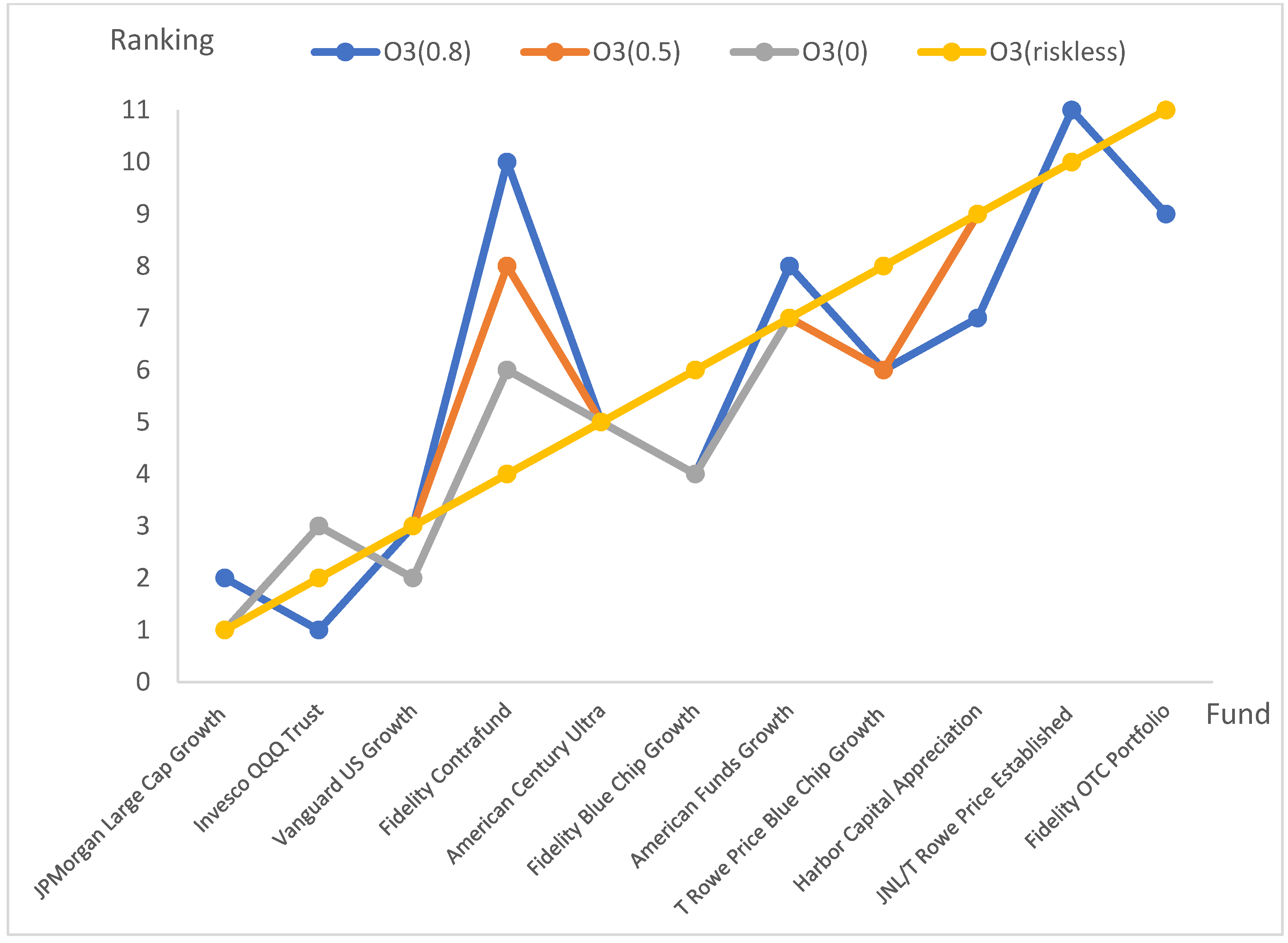
Figure 1 shows the ranking of the eleven funds according to higher-order, i.e., First, Second, and Third Omega at different thresholds. As the threshold L increases, the ranking of each fund changes. Take Fidelity as an example. It ranks the third amongst the eleven funds the according to the first-order Omega when L-riskless (which is presented by the yellow line). However, its rank becomes 11th when L= 0.5 (which is presented by the dark orange line). In the previous section, we have demonstrated the consistency between the ANSD and higher-order Omega ranking. It is critical to specify L as described in Section 3 to hold such consistency.
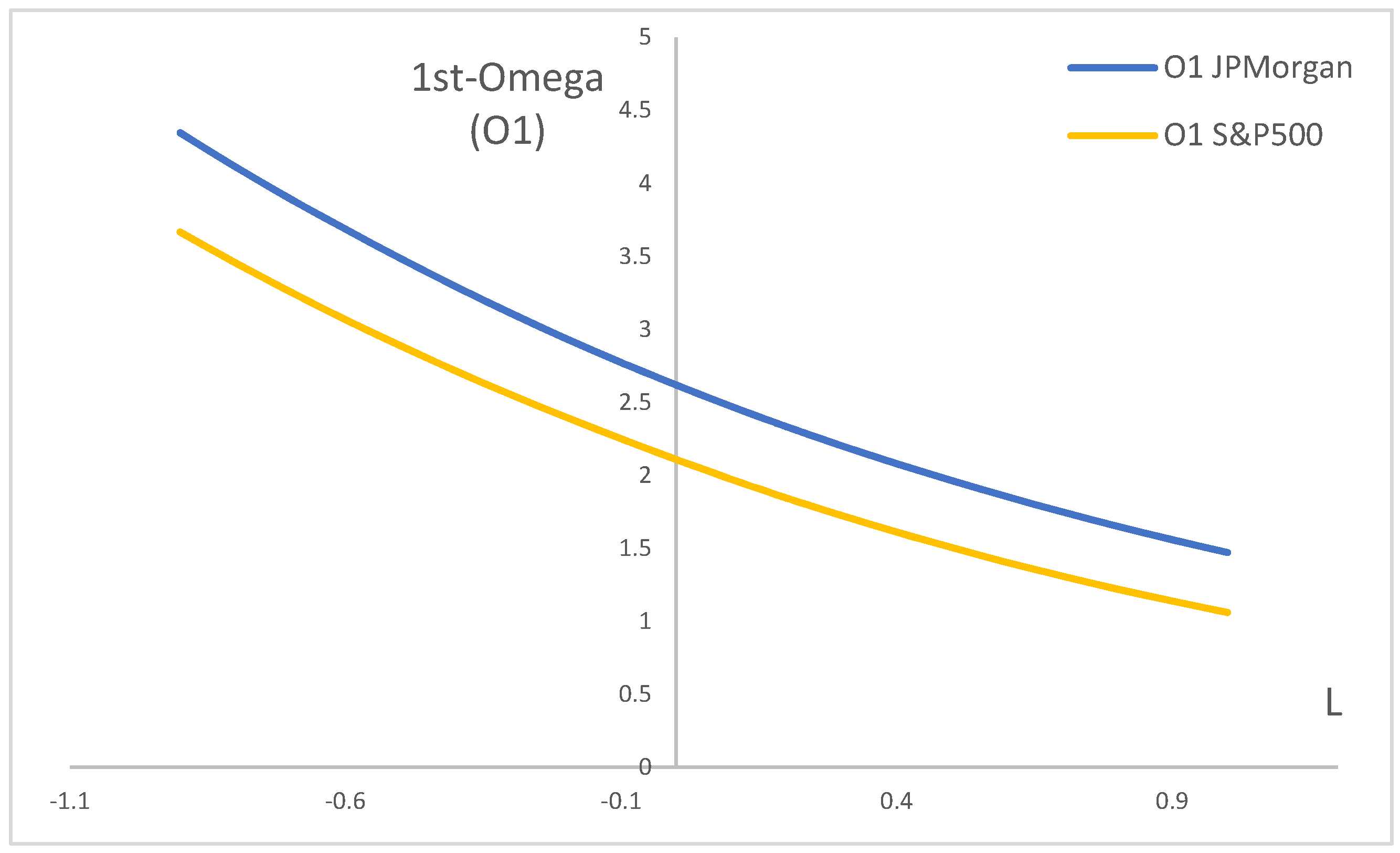
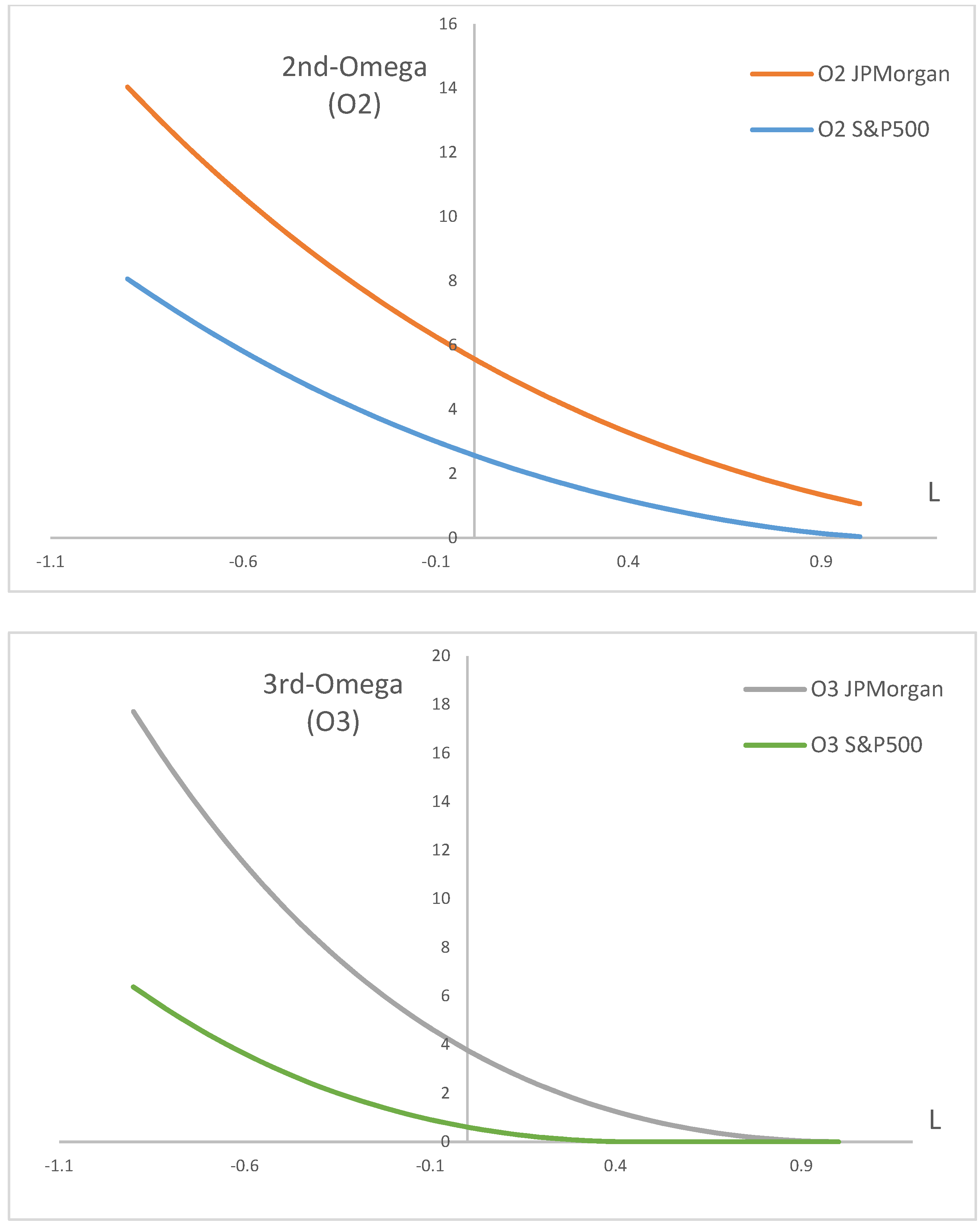
In order to further clarify the impact of threshold on the value of Omega and rankings of the evaluated fund, we now take one random fund, for example, JPMorgan Large Cap and compare it with S&P500. Figure 2 plots the Nth-order Omega at different thresholds. Obviously, Omega is a monotonic function with threshold L, and as L increases, the value of Omega becomes smaller. As seen in Figure 2, the Omega of JPMorgan is always greater than S&P500, and as the threshold continues to increase, the differences between the two becomes smaller.

5. Conclusions and Remarks

Higher-order Omega is an extension based on the Omega function proposed by Keating and Shadwick (2002). Previous literature has proved the relationship between the Nth-order Omega and the Nth-degree Stochastic Dominance. It is shown that there is one-to-one consistency between the higher-order Stochastic Dominance and the same-order Omega (Bi et al. 2019). However, theoretical and empirical evidence show that investment decision making based on the Omega function do not always reflect the Nth-degree Stochastic Dominance relationship between funds. The consistency of Stochastic Dominance and Nth-order Omega is severely limited in practical applications. To solve this problem, we turn to Almost Stochastic Dominance.
We find that, under certain conditions, Nth-degree Almost Stochastic Dominance between two portfolios is always consistent with their Nth-order Omega ordering. The First-order Omega is consistent with Almost First-order Stochastic Dominance when the threshold is in L 1 , L 2 , and L 1 and L 2 are as the Almost First-order Stochastic Dominance critical value changes. This remains true when N is greater than 1. We also use First-order Omega, Second-order Omega, and Third-order Omega to evaluate eleven U.S. funds’ performance and compare it with the ranking based on the Sharpe ratio. It is found that the rankings based on the Sharpe ratio and Omega are slightly different, and the ranking results between different orders of Omega are not consistent. There is no Stochastic Dominance relationship between the two funds, but there is always an Almost Stochastic Dominance relationship at higher order. The Almost Nth-order Stochastic Dominance relationship is consistent with the same order of Omega ranking, which provides support for our theoretical proof.
Our findings break through the limitations of the original consistency relationship between the higher-order Omega and Nth-degree Stochastic Dominance, address the partial ordering problem of Almost Stochastic Dominance, and confirm the wider use of higher-order Omega significantly. The consistency of higher-order Omega and Almost Nth-degree Stochastic Dominance is more plausible than with Stochastic Dominance. Compared to Stochastic Dominance, there is always an Almost Stochastic Dominance relation between the two portfolios corresponding to the degree no matter the N value. This study also clarifies the impact of the threshold value L in the ratio on the fund performance ranking, i.e., as the L increases the value of Omega decreases. Hence, it is critical to specify the L so that the consistency holds.
In the future, we would like to integrate the utility conditions into the definition of Almost Stochastic Dominance and the characteristics of the higher-order Omega. This will allow us to optimize the mathematical conditions of the consistency relationship between them in order to advance the application of higher-order Omega as a state-of-the-art fund evaluation index. Huang et al. (2022) constructed upper partial moment- (UPM) and lower partial moment (LPM)-based indexation strategies, which outperform traditional indexation strategies. As stated in the Introduction, the Omega ratio is obtained by dividing the first-order UPM by the first-order LPM. Hence, it is worth applying the higher-order Omega to develop innovative investment strategies.

Author Contributions

All authors contributed to the study’s conception and design. Material preparation, data collection and analysis were performed by H.L. and Y.Z. The first draft of the manuscript was written by H.L. and all authors commented on previous versions of the manuscript. All authors have read and agreed to the published version of the manuscript.

Funding

This research was funded by Major Projects of Philosophy and Social Science Research of Jiangsu universities (2022SJZD049) and Fundamental Research Funds for the Central Universities (ND2021003).

Conflicts of Interest

The authors have no relevant financial or non-financial interest to disclose.

Appendix A

Proof of Proposition 2.
 
If X S S D Y , Ω X 2 L Ω Y 2 L .
x , y a , b , F X , F Y are CDFs and F X 2 , F Y 2 are second-order integrals.
CDF of L, O x = 1 x L ,   O 2 x = L x O 1 t d t = x L , f o r   x L .
According to properties of CDF: x , y a , b , 0 F X , F Y 1 ,
F X 2 = F X 0 , F Y 2 = F Y 0 , we could have that F X 2 , F Y 2 are monotonically non-decreasing and convex functions.
We can derive F X 2 , F Y 2 0 from above.
F X 2 , F Y 2 intersect O 2 x at s X 2 , s Y 2 , and L s X 2 s Y 2 b . Here is a short proof as follows.
There exists only one constant L makes F x O x = 0 , hence there are at most two points that make F 2 x O 2 x = 0 .
Assume there are three or more points, make F 2 x O 2 x = 0 . For example, there are points η 1 < η 2 < η 3 . From Mean Value Theorem for Integration, we know that,
x 1 η 1 , η 2 , η 1 η 2 F x O x d x = η 2 η 1 F x 1 O x 1 ,
Rewrite it as
0 = F 2 η 2 O 2 η 2 F 2 η 1 O 2 η 1 = η 2 η 1 F x 1 O x 1 ,
η 2 η 1 0 , therefore, F x 1 O x 1 = 0 . Similarly, x 2 η 2 , η 3 , make F x 2 O x 2 = 0 .
Only one constant L makes F L O L = 0 , so x 1 = x 2 = L , but x 1 x 2 is a contradiction.
In a word, there are at most two points that make F 2 x O 2 x = 0 , and the two points are on both sides of L. For x < L , O 2 x 0 and F 2 x 0 , they intersect at 0. However, this intersection is meaningless. For x L , O 2 x = x L ,   F 2 x intersects O 2 x only once and F 2 b < O 2 b .
Then we assume F X 2 , F Y 2 intersect O 2 x at s X 2 , s Y 2 , According to Definition 3, If X S S D Y ,
F X 2 φ F Y 2 φ
s X 2 s Y 2 if not, F Y 2 s X 2 > F X 2 s X 2 = O 2 s X 2 , which contradicts with F 2 b < O 2 b .
Given the above, L s X 2 s Y 2 b holds.
Next, we will explain Proposition 2,
Ω X 2 L = F X 2 O 2 O 2 φ F X 2 φ d φ F X 2 > O 2 F X 2 φ O 2 φ d φ = s X 2 b O 2 φ F X 2 φ d φ a s X 2 F X 2 φ O 2 φ d φ
Ω Y 2 L is calculated similarly.
Ω Y 2 L = F Y 2 O 2 O 2 φ F Y 2 φ d φ F Y 2 > O 2 F Y 2 φ O 2 φ d φ = s Y 2 b O 2 φ F Y 2 φ d φ a s Y 2 F Y 2 φ O 2 φ d φ
According to L s X 2 s Y 2 b and (A1),
When φ s X 2 , b , O 2 φ F X 2 φ 0 and it will increase as φ ;
When φ s Y 2 , b , O 2 φ F X 2 φ O 2 φ F Y 2 φ 0 . So,
s X 2 b O 2 φ F X 2 φ d φ s Y 2 b O 2 φ F X 2 φ d φ s Y 2 b O 2 φ F Y 2 φ d φ ,
Similarly,
a s X 2 F X 2 φ O 2 φ d φ a s X 2 F Y 2 φ O 2 φ d φ a s Y 2 F Y 2 φ O 2 φ d φ ,
Therefore,
s X 2 b O 2 φ F X 2 φ d φ a s X 2 F X 2 φ O 2 φ d φ s Y 2 b O 2 φ F Y 2 φ d φ a s Y 2 F Y 2 φ O 2 φ d φ
That is, Ω X 2 L Ω Y 2 L . □

Appendix B

Proof of Proposition 3.
 
If X N S D Y , Ω X N L Ω Y N L .
x , y a , b , F X , F Y are CDFs and F X N , F Y N are second-order integrals.
CDF of L, O x = 1 x L , O N x = L x O N 1 t d t = x L , f o r   x L .
The proof is similar to N = 2. We make a simple description as,
x , y a , b , 0 F X , F Y , O x 1 , F X N , F Y N , O N x are non-negative and non-decreasing monotonical functions.
F X N , F Y N intersect O N from above once at S X N , S Y N when F X N b , F Y N b O N b (from Bi et al. 2019):
F X N O N O N φ F X N φ d φ F Y N O N O N φ F Y N φ d φ ,
and F X N O N F X N φ O N φ d φ F Y N O N F Y N φ O N φ d φ .
Therefore, Ω X N L Ω Y N L . □

Appendix C

Proof of Theorem 1.
 
When L L 1 , L 2 , if X A F S D Y , Ω X 1 L Ω Y 1 L .
x , y a , b , F X , F Y are CDFs and F X 1 , F Y 1 are first-order integrals. According to properties of CDF: x , y a , b , 0 F X 1 , F Y 1 1 , and both are monotonical and non-decreasing functions.
CDF of L, O 1 x = 1 x L .
F X 1 , F Y 1 intersect O 1 x once at s X * , s Y * and we know from Bi et al. (2019), s X * = L , s Y * = L .
Define U L = a , L , U H = L , b .
U 1 = x a , b | F X 1 φ F Y 1 φ , U 2 = x a , b | F X 1 φ > F Y 1 φ , M = U 1 F Y 1 φ F X 1 φ d φ , N = U 2 F X 1 φ F Y 1 φ d φ . M 1 = U 1 U L F Y 1 φ F X 1 φ d φ , M 2 = U 1 U H F Y 1 φ F X 1 φ d φ , N 1 = U 2 U L F X 1 φ F X 1 φ d φ , N 2 = U 2 U H F X 1 φ F Y 1 φ d φ , M 1 + M 2 = M ,   and   similarly ,   N 1 + N 2 = N .
If X A F S D Y :
U 2 F X 1 φ F Y 1 φ d φ | F Y 1 φ F X 1 φ | d φ = N M + N ε 1
Therefore, there exists a constant δ 1 = ε 1 1 ε 1 , satisfying
N δ 1 M
Denote ω 1 = L b O 1 φ F X 1 φ d φ and ω 2 = a L F X 1 φ O 1 φ d φ ,
Ω X 1 L = F X 1 O 2 O 1 φ F X 1 φ d φ F X 1 > O 1 F X 1 φ O 1 φ d φ
= U H O 1 φ F X 1 φ d φ U L F X 1 φ O 1 φ d φ
= ω 1 ω 2
Ω Y 1 L = F Y 1 O 2 O 1 φ F Y 1 φ d φ F Y 1 > O 1 F Y 1 φ O 1 φ d φ = U H O 1 φ F Y 1 φ d φ U L F Y 1 φ O 1 φ d φ = U H O 1 φ F X 1 φ d φ + U H F X 1 φ F Y 1 φ d φ U L F X 1 φ O 1 φ d φ + U L F Y 1 φ F X 1 φ d φ = ω 1 + U 2 U H F X 1 φ F Y 1 φ d φ U 1 U H F Y 1 φ F X 1 φ d φ ω 2 + U 1 U L F Y 1 φ F X 1 φ d φ U 1 U L F X 1 φ F Y 1 φ d φ = ω 1 + N 2 M 2 ω 2 + M 1 N 1
Ω X 1 L Ω Y 1 L = ω 1 ω 2 ω 1 + N 2 M 2 ω 2 + M 1 N 1 = ω 1 ω 2 + M 1 N 1 ω 2 ω 1 + N 2 M 2 ω 2 ω 2 + M 1 N 1 = ω 1 M 1 N 1 ω 2 N 2 M 2 ω 2 ω 2 + M 1 N 1
Due to the definition of Nth-order Omega, ω 2 ω 2 + M 1 N 1 > 0 .
The Theorem 1 to be proved is equivalent to this,
Ω X 1 L Ω Y 1 L 0 , ω 1 M 1 N 1 ω 2 N 2 M 2 0 ( B )
Then in three following cases:
  • If M 1 > N 1 ,
    N 2 > M 2 ,
    When ω 1 ω 2 , we can conclude M 1 N 1 > N 2 M 2 > 0 from (A1), so,
    ω 1 M 1 N 1 > ω 2 N 2 M 2 .
    (B) holds.
    When ω 1 < ω 2 ,
    ω 1 M 1 N 1 ω 2 N 2 M 2 > ω 1 M 1 ω 2 N 1 ω 2 N 2 + ω 1 M 2 = ω 1 M ω 2 N ,
    Furthermore, N δ 1 M ,
    ω 1 M ω 2 N ω 1 M ω 2 δ 1 M 0 , ω 1 ω 2 δ 1
    There exists a constant L 1 such that,
    L 1 b O 1 φ F X 1 φ d φ a L 1 F X 1 φ O 1 φ d φ = δ 1 ,
    Omega is a monotone function of return threshold L, if L L 1 , (*) holds..
    Therefore, if N 2 > M 2 , (*) holds when L L 1 , (*) holds.
    N 2 M 2 , ω 1 M 1 N 1 > 0 , ω 2 N 2 M 2 > 0 .
    (B) holds.
  • If M 1 = N 1 ,
    ω 1 M 1 N 1 ω 2 N 2 M 2 = ω 2 N 2 M 2 = ω 2 N N 1 M M 1 = ω 2 N M > 0 .
    (B) holds.
  • If M 1 < N 1 , then M 2 > N 2 ,
    When ω 1 ω 2 , we can conclude M 2 N 2 > N 1 M 1 > 0 from (A1), so,
    ω 2 M 2 N 2 > ω 1 N 1 M 1 ,
    (B) holds.
    When ω 1 > ω 2 ,
    ω 1 M 1 N 1 ω 2 N 2 M 2 > ω 2 M 1 ω 1 N 1 ω 1 N 2 + ω 2 M 2 = ω 2 M ω 1 N
    Furthermore, N δ 1 M ,
    ω 2 M ω 1 N ω 2 M ω 1 δ 1 M 0 , ω 1 ω 2 1 δ 1
    There exists a constant L 2 such that,
    L 2 b O 1 φ F X 1 φ d φ a L 2 F X 1 φ O 1 φ d φ = 1 δ 1 ,
    Omega is a monotone function of return threshold L, if L L 2 , (*) holds.
Therefore, if M 1 < N 1 , M 2 > N 2 , (*) holds when L L 2 . □
For all three possible cases, we obtain that there exists constant L 1 , L 2 such that,
If X A F S D Y , Ω X 1 L Ω Y 1 L when L L 1 , L 2 .

Appendix D

Proof of Theorem 2.
 
When L N L 1 N , L 2 N , If X A N S D Y , Ω X N L Ω Y N L .
(1) x , y a , b , 0 F X , F Y , O x 1 , F X N , F Y N , O N x are non-negative and non-decreasing monotonical function.
(2) F X N b , F Y N b O N , intersects only once at s X N , s Y N L .
Assume s X N < s Y N as an example.
Figure A1. O(x), F X , F Y are Cumulative Distribution Functions (CDFS). Note: X-axis shows the threshold. Y-axis shows the value of CDFs. F X , F Y intersect O(x) at S X , S Y , and L S X , S Y b .
Jrfm 15 00438 g0a1
Define U L N = a , S X N , U M N = S X N , S Y N , U H N = S Y N , b .
U 1 N = x a , b | F X N φ F Y N φ ,   U 2 N = x a , b | F X N φ > F Y N φ . C N = U 1 N F Y N φ F X N φ d φ , C 1 N = U 1 N U L N F Y N φ F X N φ d φ + U 1 N U M N F Y N φ O N φ d φ , C 2 N = U 1 N U H N F Y N φ F X N φ d φ + U 1 N U M N O N φ F Y N φ d φ , C 1 N + C 2 N = C N ; V N = U 2 N F X N φ F Y N φ d φ , V 1 N = U 2 N U L N F X N φ F Y N φ d φ , V 2 N = U 2 N U H N F X N φ F Y N φ d φ ,
And + V 2 N = V N .
If X A N S D Y :
V N C N + V N = U 2 N F X N φ F Y N φ d φ F Y N φ F X N φ d φ ε N ,
Therefore, there exists a constant making V N δ N * C N , and δ N = ε N 1 ε N .
Denote
ω 1 N = S X N b O N φ F X N φ d φ   a n d   ω 2 N = a S X N F X N φ O N φ d φ , Ω X N L = F X N O N O N φ F X N φ d φ F X N > O N F X N φ O N φ d φ = ω 1 N ω 2 N Ω Y N L = F Y N O N O N φ F Y N φ d φ F Y N > O N F Y N φ O N φ d φ = ω 1 N + V 2 N C 2 N ω 2 N + C 1 N V 1 N Ω X N L Ω Y N L = ω 1 N ω 2 N ω 1 N + V 2 N C 2 N ω 2 N + C 1 N V 1 N = ω 1 N ω 2 N + C 1 N V 1 N ω 2 N ω 1 N + V 2 N C 2 N ω 2 N ω 2 N + C 1 N V 1 N = ω 1 N C 1 N V 1 N ω 2 N V 2 N C 2 N ω 2 N ω 2 N + C 1 N V 1 N
The proof is similar to N = 1, and we conclude that,
When L N L 1 N , L 2 N , Ω X N L Ω Y N L 0 holds, where. Ω X N L 1 N = δ N , Ω X N L 2 N = 1 δ N .
In conclusion, If X A N S D Y , Ω X N L Ω Y N L , with L N L 1 N , L 2 N . □

References

  1. Bai, Zhidong, Li Huai, McAleer Michael, and Wong Wing-Keung Wong. 2015. Stochastic Dominance Statistics for Risk Averters and Risk Seekers: An Analysis of Stock Preferences for USA and China. Quantitative Finance 15: 889–900. [Google Scholar] [CrossRef]
  2. Balder, Sven, and Nikolaus Schweizer. 2017. Risk aversion vs. the Omega ratio: Consistency results. Finance Research Letters 21: 78–84. [Google Scholar] [CrossRef]
  3. Bali, Turan G., Stephen J. Brown, and K. Ozgur Demirtas. 2013. Do hedge funds outperform stocks and bonds. Management Science 59: 1887–903. [Google Scholar] [CrossRef]
  4. Bellini, Fabio, Bernhard Klar, and Alfred Muller. 2016. Expectiles, Omega Ratios and Stochastic Ordering. Methodology and Computing in Applied Probability 20: 855–73. [Google Scholar] [CrossRef]
  5. Benhamou, Eric, Beatrice Guez, and Nicolas Paris. 2019. Omega and Sharpe ratio. Social Science Research Network (SSRN) Working Paper. [Google Scholar] [CrossRef]
  6. Bi, Hongwei, Rachel J. Huang, Larry Y. Tzeng, and Wei Zhu. 2019. Higher-order Omega: A performance index with a decision-theoretic foundation. Journal of Banking and Finance 100: 43–57. [Google Scholar] [CrossRef]
  7. Caporin, Massimiliano, Michele Costola, Gregory Jannin, and Bertrand B. Maillet. 2018. On the (Ab)use of Omega? Journal of Empirical Finance 46: 11–33. [Google Scholar] [CrossRef]
  8. Chan, Stephen, and Saralees Nadarajah. 2019. Risk: An R package for financial risk measures. Computational Economics 53: 1337–51. [Google Scholar] [CrossRef]
  9. Davidson, Russell, and Jean-Yves Duclos. 2000. Statistical inference for stochastic Dominance and the measurement of poverty and inequality. Econometrica 68: 1435–64. [Google Scholar] [CrossRef]
  10. Fong, Wai Mun. 2016. Stochastic Dominance and the omega ratio. Finance Research Letters 17: 7–9. [Google Scholar] [CrossRef]
  11. Guidolin, Massimo, and Allan Timmermann. 2008. International asset allocation under regime switching, skew, and kurtosis preference. Review of Financial Studies 21: 889–935. [Google Scholar] [CrossRef]
  12. Guo, Xu, Haim Levy, Lu Richard, and Wing-Keung Wong. 2018. Could Omega ratio perform better than Sharpe ratio? Social Science Research Network (SSRN) Working Paper. [Google Scholar] [CrossRef]
  13. Guo, Xu, Xuejun Jiang, and Wing-Keung Wong. 2017. Stochastic Dominance and Omega Ratio: Measures to Examine Market Efficiency, Arbitrage Opportunity, and Anomaly. Economies 5: 38. [Google Scholar] [CrossRef]
  14. Harvey, Campbell R., and Akhtar Siddique. 2000. Conditional skewness in asset pricing tests. The Journal of Finance 55: 1263–95. [Google Scholar] [CrossRef]
  15. Heufer, Jan. 2014. Generating random optimising choices. Computational Economics 44: 295–305. [Google Scholar] [CrossRef]
  16. Huang, Jinbo, Yong Li, and Haixiang Yao. 2022. Partial moments and indexation investment strategies. Journal of Empirical Finance 67: 39–59. [Google Scholar] [CrossRef]
  17. Kaplan, Paul D., and James A. Knowles. 2004. Kappa: A generalised downside risk-adjusted performance measure. Journal of Performance Measure 8: 42–54. Available online: http://w.performance-measurement.org/KaplanKnowles2004.pdf (accessed on 2 July 2022).
  18. Keating, Con, and William F. Shadwick. 2002. A Universal Performance Measure. Journal of Performance Measure 6: 59–84. Available online: https://oxfordstrat.com/coasdfASD32/uploads/2016/03/A-Universal-Performance-Measure.pdf (accessed on 2 July 2022).
  19. Klar, Bernhard, and Alfred Müller. 2018. On Consistency of the Omega Ratio with Stochastic Dominance Rules. World Scientific Book Chapters. Innovations in Insurance, Risk- and Asset Management, chapter 14. Edited by Kathrin Glau, Daniël Linders, Aleksey Min, Matthias Scherer, Lorenz Schneider and Rudi Zagst. Singapore: World Scientific Publishing Co. Pte. Ltd., pp. 367–80. [Google Scholar]
  20. Leshno, Moshe, and Haim Levy. 2010. Economically relevant preferences for all observed epsilon. Annals of Operational Research 176: 153–78. [Google Scholar] [CrossRef]
  21. Levy, Haim. 2015. Stochastic Dominance: Investment Decision Making under Uncertainty, 3rd ed. New York: Springer. [Google Scholar]
  22. Muller, Alfred, Marco Scarsini, Ilia Tsetlin, and Robert L. Winkler. 2017. Between first and second-order stochastic dominance. Management Science 48: 1074–85. [Google Scholar] [CrossRef]
  23. Sharpe, William. 1966. Mutual Fund Performance. The Journal of Business 39: 119–38. [Google Scholar] [CrossRef]
  24. Stutzer, Michael. 2000. A Portfolio Performance Index. Financial Analysts Journal 56: 52–61. [Google Scholar] [CrossRef] [Green Version]
  25. Treynor, Jack L. 1965. How to Rate Management of Investment Funds. Harvard Business Review 43: 63–75. [Google Scholar]
  26. Tzeng, Larry Y., Rachel J. Huang, and Pai-Ta Shih. 2013. Revisiting almost second-degree stochastic Dominance. Management Science 59: 1250–54. [Google Scholar] [CrossRef]
  27. van Dyk, Francois, Gary van Vuuren, and Andre Heymans. 2014. Hedge Fund Performance Evaluation Using the Sharpe and Omega Ratios. International Business & Economics Research Journal 13: 485–512. [Google Scholar] [CrossRef]
  28. Yang, Han, Ming-Hui Wang, and Nan-Jing Huang. 2021. The alpha α-Tail Distance with an Application to Portfolio Optimization Under Different Market Conditions. Computational Economics 58: 1195–224. [Google Scholar] [CrossRef]
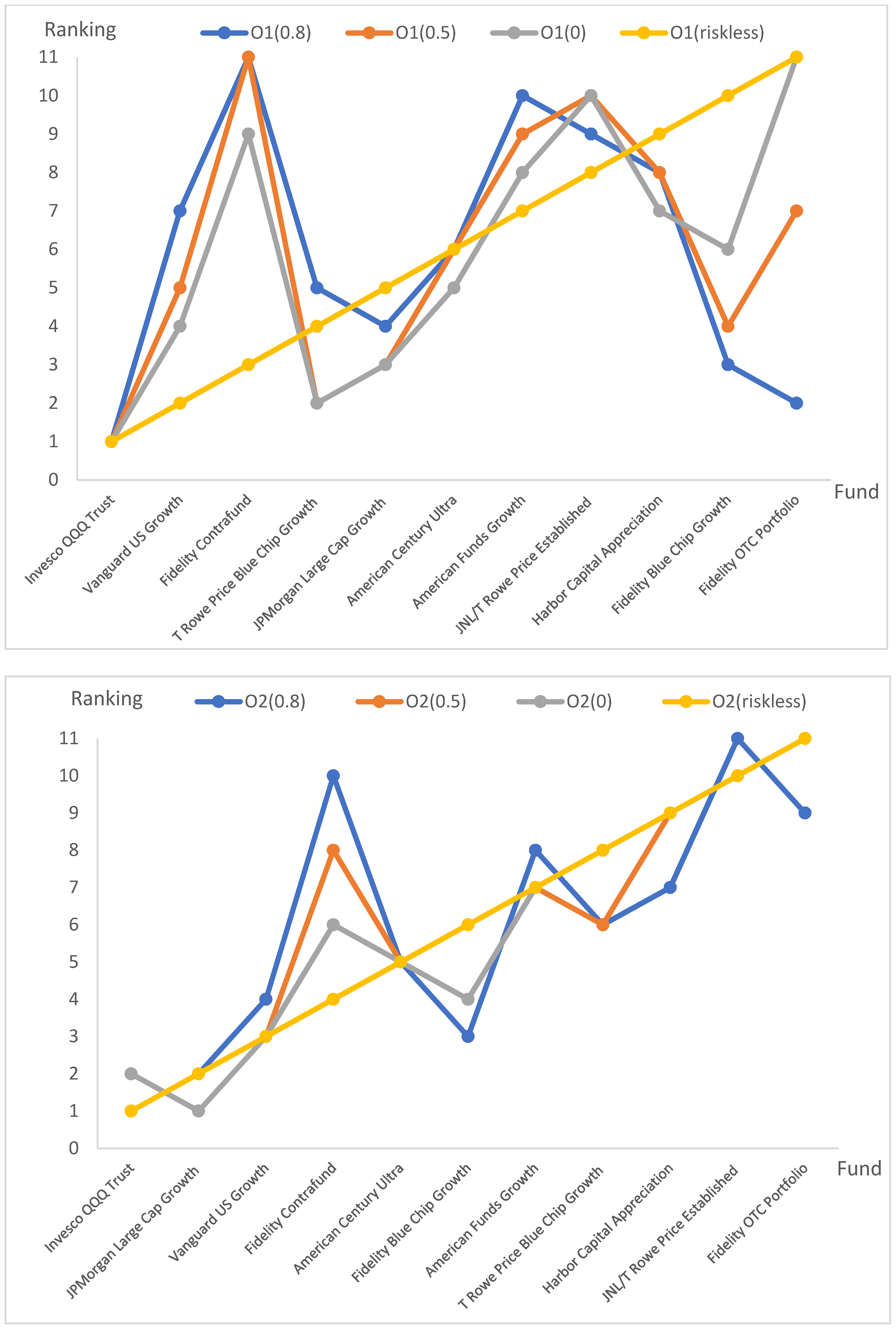
Figure 1. The 1st-, 2nd-,3rd-order Omega rankings at different thresholds. Note: X-axis shows the eleven funds’ ranking when the L = riskless rate at different order of Omega. Y-axis shows the ranking when L = 0.8, 0.5, 0, and riskless respectively.
Jrfm 15 00438 g001aJrfm 15 00438 g001b
Figure 2. 1st-, 2nd-,3rd-order Omega as a monotone function of return threshold.
Jrfm 15 00438 g002aJrfm 15 00438 g002b
Table 1. Descriptive Statistics of the eleven funds’ monthly return.
Fund NameMean Return (%)Standard DeviationSkewnessKurtosis
American Century Ultra1.6111 4.4748 0.0048 1.1547
American Funds Growth1.4790 4.1604 −0.1610 1.3951
Fidelity Blue Chip Growth1.7089 4.6816 −0.0649 1.0033
Fidelity Contrafund1.4121 3.9989 −0.0879 1.1835
Fidelity OTC Portfolio1.7774 5.0226 −0.2042 0.5733
Harbor Capital Appreciation1.6457 4.6096 −0.0895 0.6735
Invesco QQQ Trust1.7948 4.4728 0.0079 0.3949
JNL/T Rowe Price Established 1.5354 4.4444 −0.0933 1.1473
JPMorgan Large Cap Growth 1.6673 4.6173 0.0976 1.2822
T Rowe Price Blue Chip Growth 1.6300 4.4352 −0.0242 0.9554
Vanguard US Growth1.6277 4.4806 −0.0023 1.2025
Table 2. The 1st-, 2nd-,3rd-order Omega and Sharpe Ratio.
Fund Name Ω F 1 (Riskless) Ω F 2 (Riskless) Ω F 3 (Riskless)Sharpe Ratio
Fidelity Blue Chip Growth3.9885(5)11.2800(2)11.9774(2)0.5382(3)
Fidelity OTC Portfolio3.6151(6)7.8487(6)5.9280(6)0.5152(6)
Harbor Capital Appreciation 3.9998(4)9.6957(4)8.7164(4)0.5328(4)
Invesco QQQ Trust 4.3541(1)13.0826(1)14.6950(1)0.5825(1)
JNL/T Rowe Price Established 4.0157(3)9.5737(5)8.5982(5)0.5278(5)
T Rowe Price Blue Chip Growth 4.2241(2)10.9485(3)10.9183(3)0.5502(2)
Table 3. Almost First Stochastic Dominance (AFSD) test results.
JNL/T Rowe Price EstablishHarbor Capital AppreciationFidelity Blue Chip Growth
JNL/T Rowe Price Establish
Harbor Capital Appreciation0.0021 < ε 1 *
Fidelity Blue Chip Growth0.0065 < ε 1 * 0.0000 < ε 1 *
Note: If the value ε < ε N * , it is shown that the fund in a row dominated the funds in a column. Refer to Leshno and Levy (2010), ε 1 * = 5.9 % . In this AFSD test, the AFSD ranking is JNL/T Rowe Price Establish > Harbor Capital Appreciation > Fidelity Blue Chip Growth, which is consistent with the First-order Omega ranking.
Table 4. Almost Second Stochastic Dominance (ASSD) test results.
Invesco QQQ TrustT Rowe Price Blue Chip GrowthHarbor Capital Appreciation Fidelity OTC Portfolio
Invesco QQQ Trust
T Rowe Price Blue Chi 0.0000 < ε 2 *
Harbor Capital Apprec 0.0000 < ε 2 * 0.0000 < ε 2 *
Fidelity OTC Portfolio0.0000 < ε 2 * 0.0000 < ε 2 * 0.0000 < ε 2 *
Note: If the value ε < ε N * , it is shown that the fund in a row dominated the funds in a column. Refer to Leshno and Levy (2010), ε 2 * = 3.2 % . In this ASSD test, the ASSD ranking is Invesco QQQ Trust > T Rowe Price Blue Chip Growth > Harbor Capital Appreciation > Fidelity OTC Portfolio, which is consistent with the Second-order Omega ranking.
Publisher’s Note: MDPI stays neutral with regard to jurisdictional claims in published maps and institutional affiliations.