Improvement of Service Quality in the Supply Chain of Commercial Banks—A Case Study in Vietnam

Abstract

The outbreak of the Covid-19 pandemic caused a serious impact on the business activities of enterprises and households, affecting the operation of banks around the world, especially for capital mobilization from those with savings deposits at commercial banks. In face of the unpredictable developments of the pandemic, many services of banks in Vietnam were also affected, so it has been necessary to make a plan to maintain business operations and respond effectively to these difficulties. In this study, the authors used three research models to form a three-dimensional frame of reference (past, present, and future) to identify, analyze, and evaluate the factors affecting the service quality of commercial banks’ savings deposit mobilization, and to suggest solutions that can minimize risks and improve customer satisfaction for savings deposits at commercial banks, improve service quality to avoid potential long-term risks, as well as maintain sustainable growth and social stability in the future.

1. Introduction

Vietnam is the third most populous country in Southeast Asia and ranks 15th in the world in population, and the average life expectancy is more than 73 years. With a total population of more than 96 million people, Vietnam is at the stage of the “gold” population structure (20–44 years old), but only 60% of the population aged 15 and over own a bank account (Thu Hoa 2020). Over the past 10 years, the leaders of Vietnam’s commercial banks have been changing their strategies to focus on more exploitation of retail activities. This strategy aims to diversify revenue sources, minimize operational risks, and achieve the best business efficiency.

Vietnam currently has more than 30 domestic banks and more than 60 banks and branches that are 100% foreign-owned, representative offices of foreign banks in Vietnam. Furthermore, because of the simplicity of retail capital mobilization in terms of both techniques and operations, most banks have carry it out. People have a lot of options when selecting a bank for savings. Furthermore, in recent years, the race to attract demand deposit resources is booming among banks, because this service reflects the efficiency of providing comprehensive banking and financial services, especially attracting customers to use digital banking services.

Furthermore, the role of financial services is to facilitate customers in savings and other service providers in managing information and financial flows. Banks are used to keeping customers’ savings and are providers of payment management and service supply that integrate material and financial supply chains (Figure 1). Banks can promote supply chain coordination, collaboration, information sharing, and visibility to support customers. When customers have greater knowledge about the bank’s service packages before making a transaction, they can avoid risks and have better opportunities with these service packages. Thereby, cooperation between customers and banks in the service supply chain at commercial banks can be improved. In the banking sector, customer service plays an extremely important role. Service quality is a measure to reflect the bank’s overall business. If the quality of customer service is good and demonstrates professionalism, customers will trust and perform transactions at that bank. On the contrary, poor customer service will make customers to refuse the products and services provided by the bank, which will greatly affect the business situation of commercial banks.

The authors conducted a case study at a big commercial bank in Vietnam that has a full range of capital mobilization, lending, guarantee, payment, foreign currency trading, remittance services, financial consulting, and other banking services. In this study, the authors examined the factors affecting the satisfaction of customers when using services at banks. Additionally, the authors identified the factors affecting the early withdrawal of savings at banks, in order to propose reasonable solutions for both customers and managers at banks. In addition, in this study, the authors used the Gray forecasting model to forecast the main business indicators of commercial banks to help the bank be well prepared to serve customers better, to improve customer service performance and customer service quality, and to help commercial banks stabilize their business situation and develop sustainably.

2. Literature Review

Anand and Selvaraj (2013) used the Servperf model to measure service quality and the factors affecting customer satisfaction in Indian banks using the following six (6) factors that they hypothesized would affect customer satisfaction: (1) tangibles, (2) reliability, (3) responsiveness, (4) assurance, (5) empathy, and (6) service capacity. The results of the study indicated that customer satisfaction was influenced by the following four (4) factors: (1) empathy, (2) responsiveness, (3) tangibles, and (4) service capacity (Anand and Selvaraj 2013). The study also shows that empathy and responsiveness in public and private sector banks have a strong impact on satisfaction. Meanwhile, in the Indian Postal Savings Bank, responsiveness and tangibles were the factors with the strongest impact on customer satisfaction.

Ahmed (2017) measured the service quality of banks in Pakistan based on the Servqual model of Parasuraman et al. (1985) for research objects such as Islamic banks (38.40%) and normal commercial banks (61.60%) (Ahmed 2017). The author proposed a model of a service quality dependent variable affected by (1) tangibles, (2) reliability, (3) convenience, (4) service capacity, and (5) satisfaction, that have an impact on the service quality of banks in Pakistan. Drawing from 250 valid surveys for data processing (reliability test, correlation, and analysis of regression models), the author concluded that the proposed Servqual model was suitable for the measurement of the service quality. All five independent variables were important for the improvement of service quality. However, in the case of Islamic banks, tangibles, reliability, and service capacity needed to be more focused. According to the results of that study, most customers were satisfied with the quality of the banking services.

Bente (2012) carried out a study to determine the factors affecting service quality in Romanian banks (Bente 2012). This study was a combination of qualitative and quantitative research to measure the relationship between service quality, customer satisfaction, and customer loyalty when using banking services in Romania. This study also applied the Servqual service quality scale of Parasuraman et al. (1985) with the five service quality factors, thereby discovering policy and governance implications for private and public banks in Romania to improve service quality. Chandra and Neelankavil (2008) studied customer needs and proposed solutions to help businesses successfully develop new products in developing countries. Wang et al. (2019) and colleagues used the DEA and GM (1,1) models to evaluate the effect of foreign direct investment on economic growth in developing countries.

In addition, many researchers have been using the Binary Logistic model and Grey forecasting model to conduct valuable studies for countries around the world (Wood 2006; Al Nageim et al. 2007; Chen et al. 2008; Ke 2013; Li et al. 2014; Oguz and Assefa 2014; De Gaetano 2018; Xuemei et al. 2019; Karimi and Hojati 2020; Li et al. 2021; Shetty and Vincent 2021; Durst and Gerstlberger 2021). Several outstanding research works such as Cristian et al. (2020) have employed the Binary Logistic model to study the factors affecting the feasibility and competitive advantage of enterprises in the field of transportation and supply chain. The results of this study indicated that the most important factor in selecting a digital freight forwarder is the existence of both sales and coordination departments. Barnieh et al. used the Binary Logistic model to investigate the relationships and interactions among the driven factors and responses of natural vegetation in West Africa. This result greatly contributed to the planning of programs for climate change adaptation and sustainable development in West Africa. Nguyen (2020) applied the Grey forecasting model to find solutions to improve the quality in the field of construction investment and urban development. Wang et al. (2017) used the Grey forecasting model and optimal mathematical models to research and select the partners for textile enterprises in Vietnam. The results of that study showed that textile enterprises should join a strategic alliance to enhance their strengths and develop sustainably.

However, in these studies, the researchers used a Binary Logistic model and a Grey forecasting model to research many different fields of life, but none combined qualitative and quantitative models to evaluate the services of commercial banks. In this study, the authors used a three-dimensional frame of reference including the past, present, and future. Thereby, managers of commercial banks have a full and comprehensive view of the service packages of commercial banks from which to make decisions to plan, develop strategies, and consult customers about savings at commercial banks in order to create the best efficiency for the integration of material and financial supply chains.

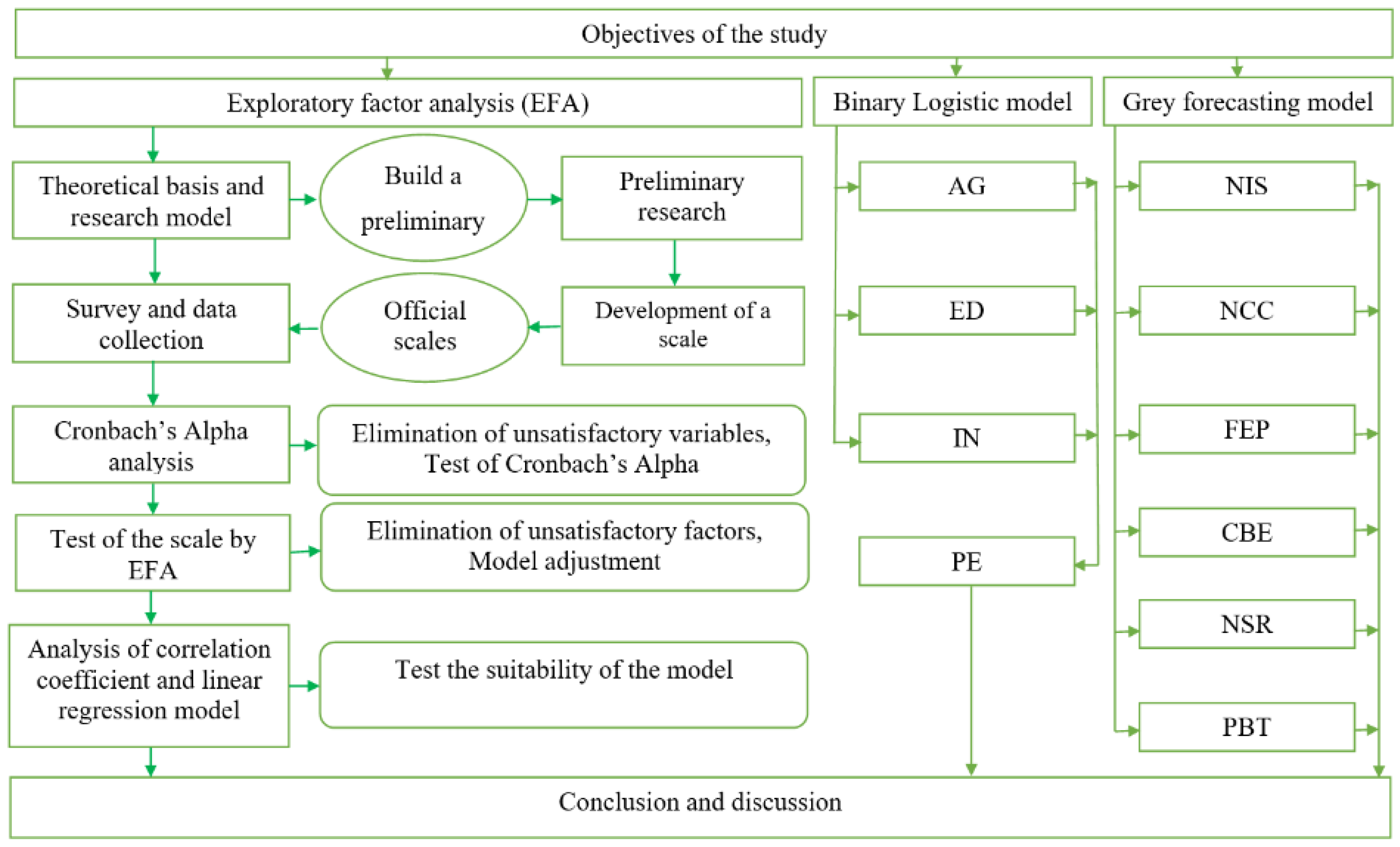
3. Research Development and Methods

After the determination of the research objectives and questions, based on theory and previous successful studies, we proposed a research model and built a preliminary scale from which to could conduct qualitative research (through group discussion) and quantitative research (test the reliability of the scale) so as to complete an official scale. Then, organized interviews with individual customers who were currently using savings deposit services at Vietnamese commercial banks were conducted, and samples were collected and data were processed using SPSS 22.0 software. The results obtained from this method were combined with the results from the Binary Logistic model and Grey forecasting model to analyze, evaluate, and recommend solutions to help managers of commercial banks successfully build and manage the integration of material and financial supply chains into their commercial banks (Figure 2).

3.1. Qualitative Research

The qualitative method was used in the first stage of the study, which mainly focused on collecting research works related to the quality of banking services as a theoretical basis to conduct group discussions, build observation variables to measure research concepts, and prepare survey questionnaires. The following Likert five-point scale was used to measure the factors to be surveyed in this study: (1) very unsatisfied, (2) unsatisfied, (3) normal, (4) satisfied, and (5) very satisfied.

3.2. Exploratory Factor Analysis

The quantitative method was used in the analysis and evaluation of the operational situation, in general, and of capital mobilization, in particular, at commercial banks. Based on the data collected from the direct surveys of customers, the authors processed the data using SPSS 22.0 software, thereby analyzing and testing the influence of the factors on the quality of the savings deposit service for individual customers.

3.2.1. Development of a Scale

Through discussions with experts in the field of commercial banking about the factors affecting the quality of personal savings deposit service, the authors constructed the factors affecting the quality of personal savings deposit services for this study.

3.2.2. Sampling Method

The authors had both worked in commercial banks for more than 15 years, so the collection of research samples was relatively convenient. Sampling was carried out using randomization. The authors randomly selected 307 samples to synthesize data so as to ensure the accuracy of the research results.

3.2.3. Data Analysis and Processing Methods

Based on the data obtained from the 307 survey samples, the authors removed the invalid ones and input them, coded and processed, using SPSS 22.0 software. The data analysis was conducted in the following steps:

Test of Cronbach’s Alpha reliability coefficient:

Cronbach’s Alpha coefficient is a statistical test that shows how closely items of the scale are correlated with each other. Variables with variable-total correlation coefficients less than 0.3 were eliminated and a scale was considered standard when its Cronbach’s Alpha reliability was 0.6 or higher (Nunnaly and Bernstein 1994).

Test of the scale by exploratory factor analysis (EFA):

Exploratory factor analysis (EFA) is a technique used mainly to simplify and summarize data after evaluating the reliability of the scale using Cronbach’s Alpha coefficient and removing the unsatisfactory variables. This method is useful for determining the set of variables to be used for the research problem as well as finding the relationship between the variables. The criteria for applying and selecting variables for exploratory factor analysis consist of the following:

Firstly, the Kaiser–Meyer–Olkin coefficient (KMO) of ≥0.5 with the Barlett significance level of ≤0.05. This was the criterion used to consider the appropriateness of EFA, and if 0.5 ≤ KMO ≤ 1, then a factor analysis is appropriate. Kaiser (1974) suggested that KMO ≥ 0.9 is very good, KMO ≥ 0.8 is good, KMO ≥ 0.7 is pass, KMO ≥ 0.6 is acceptable, KMO ≥ 0.5 is bad, and KMO 0.5 is unacceptable (Nguyen 2011).

Secondly, the factor loading was ≥0.5. This is a coefficient expressing the single correlation between variables and factors, used to evaluate the significance level of EFA (Hair et al. 2009). Factor loading > 0.3 is considered minimal, factor loading > 0.4 is considered important, and factor loading ≥ 0.5 is considered practical.

Thirdly, the scale was acceptable when the total variance extracted ≥ 50% and the eigenvalue coefficient was > 1 (Gerbing and Anderson 1988).

Fourthly, the difference in the factor loading coefficient of an observation variable between the factors was ≥0.5 to ensure the discriminant value between the factors (Jabnoun and Al-Tamimi 2003).

In the course of the EFA analysis, the authors using the principal component analysis with Varimax rotation to find the factors representing the variables and the breakpoint when extracting the factors with eigenvalues greater than 1. Varimax allowed for rotation of the factor angle to minimize the number of variables with large coefficients with the same factor, thus enhancing the ability to explain factors.

Correlation coefficient analysis:

The Pearson correlation coefficient (r) measures the linear correlation level between two variables. The Pearson correlation coefficient (r) value ranged from (−1) to (+1). The coefficient r > 0 indicates a positive correlation between two variables, which means that if the value of one increases, that of the other will also increase, and vice versa; the coefficient r < 0 indicates a negative correlation between the two variables, that is, if the value of one increases, the value of the other will decrease. With Sig. < 0.05, the higher the absolute value of r is (closer to 1), the greater the correlation level between the two variables, or, in other words, the data are completely suitable with the model (Uddin et al. 2016).

Regression analysis:

A regression analysis through SPSS 22.0 software was used to find out the correlation between the independent and dependent variables, that is, to evaluate the impact of each independent variable on the dependent variable, as well as to predict the change of the dependent variable when the independent variable changed. For research of a model with more than one independent variable, the correlation between the independent variables needs to be tested by multi-collinearity. Variance inflation factor (VIF) was used as a measure (multi-collinearity) in this regression analysis. The regression model accepts variables with a VIF of less than 10. If the VIF gives a variable in the range of a value greater than 10, it must be removed from the regression model.

Reliability (REL): When customers select a bank for deposits, reliability is one of the leading factors. In addition, clear, transparent documents; accuracy in each transaction, especially transactions for a first impression; or fulfillment of obligations and commitments that the bank has previously given, also play a very important role.

Responsiveness (RES): Measures the ability to handle customers’ problems and needs on a quick, prompt, and accurate basis.

Service capacity (SER): Shown through professional qualifications, professional service style, good communication, master of product knowledge in consulting, and professional proficiency in working.

Empathy (EMP): Shown through the attitude of the bank staff, such as kindness, warmth, thoughtfulness, and concern for the wishes and difficulties of customers.

Tangibles (TAN): Expressed through facilities, infrastructure, machinery, equipment or clothing, staff appearance, etc. What customers can see and feel with their senses.

Interest rate (INT): For savings deposits, most customers refer to interest rates when considering deposits. The main income and benefits that customers receive for the use of this service.

Customer service (CUS): Customer service is an indispensable policy for most industries and services. Therefore, concern for customers before, during, and even after a deposit contributes to an increase in benefits for customers.

3.3. Binary Logistic Model

The binary logistic model is a model used to estimate the probability of a problem (Eboli and Mazzulla 2009). The characteristic of a binary logistic model is that the dependent variable has only two values: 0 and 1. Many economic and social phenomena need to predict probability to support managers’ strategic planning for enterprises. For example, what is the possibility that customers will pay their debts on time, withdraw capital on schedule for savings accounts, or purchase products.

The factors with two such expressions encoded into two values as 0 and 1 are called binary variables. The normal regression equation cannot be analyzed when the dependent variable has more than 1 expression. The estimated regression coefficients in the binary logistic model provide the estimated change in the corresponding probability ratio between the independent and dependent variables, provided that the other independent variables remain constant. The binary logistic equation is as follows (Omondi 2019; Omondi 2021; Araveeporn 2021):

$$\begin{gathered} {\log }_e=\left[\frac{{\mathrm{P}}_i}{1-{\mathrm{P}}_i}\right]={\beta }_0+{\beta }_1{\chi }_1+{\beta }_2{\chi }_2+{\beta }_3{\chi }_3+\dots +{\beta }_k{\chi }_k \\ \{\begin{array}{l}{p}_i: \text{Probability of customers to withdraw deposit ahead of time}.\\ {\beta }_i: \text{Regression coefficient reflects the impact of the independent variables}.\end{array} \end{gathered}$$

(1)

$$\mathrm{P}=\frac{\exp ({\beta }_0+{\beta }_1{\chi }_1+{\beta }_2{\chi }_2+{\beta }_3{\chi }_3+\dots +{\beta }_k{\chi }_k)}{1+\exp ({\beta }_0+{\beta }_1{\chi }_1+{\beta }_2{\chi }_2+{\beta }_3{\chi }_3+\dots +{\beta }_k{\chi }_k)}$$

(2)

In this study, the authors used the binary logistic model to forecast and evaluate the influence of the factors including the age, education, and income of customers on the decision to withdraw capital from the bank ahead of time. From the customer’s perspective, they will have to accept the demand interest rate when withdrawing the savings deposit ahead of time, as agreed with the bank. Moreover, currently, many banks are applying a policy that disallows for partial withdrawals on the passbook. Therefore, in many cases, even though only a small portion of the total amount on the passbook is required, customers still have to accept that they must give all of the demand interest. The demand interest rate currently applied at banks is from 0.1% to 0.2% per year. Meanwhile, the lowest time interest rate is above 3%. For long terms like one year, the interest rate can be up to 7–8% per year. Thus, customers will lose a large amount that they could have enjoyed if they had withdrawn it on time for large amounts or those with a long deposit term. Thus, customers’ expectations will not be as satisfied when saving, which has a great impact on customer satisfaction about the service quality of the bank.

From the bank’s perspective, the system current commercial banks currently follow is a mechanism of internal capital transfer pricing on the principle of centralized capital management, in which the branches could be considered as intermediary for sales of capital. Of course, the interest rate difference for selling demand capital to a head office is usually higher than that for selling term capital. In the case the customer withdraws ahead of time, the branch is still profitable. However, as an enterprise in the field of currency business, the system of commercial banks needs to correspond to the maximum ratio of short-term capital used for medium- and long-term loans according to a specific route. The premature withdrawal of deposits by customers, especially for long-term deposits, may affect the capital structure of the whole system. Therefore, the premature withdrawal of deposits harms both customers and commercial banks, affecting the construction and management of supply chains integrated into material and finance in the commercial bank’s operations.

3.4. Grey Forecasting Model

Before using the Gray model, it is necessary to ensure that the original data satisfies the following formula (Nguyen 2021):

$${\partial }_{\mathrm{i}}=\frac{{\mathrm{x}}^{\left(0\right)}(\mathrm{i}-1)}{{\mathrm{x}}^{\left(0\right)}\left(\mathrm{i}\right)};(\mathrm{i}=2;3;\dots ;\mathrm{n})$$

(3)

The values of ${\partial }_i$ must be in the range of ${\partial }_{(i)}^{(0)}=({\mathrm{e}}^{-\frac{2}{n+1}};{\mathrm{e}}^{\frac{2}{n+1}})$.

Based on differential equations, make GM (1,1):

$$\frac{{\mathrm{dx}}_{(k)}^{(1)}}{\mathrm{dk}}+\mathrm{a}{x}_{(k)}^{(1)}=\mathrm{b}(\mathrm{a},\mathrm{b}\mathrm{are}\mathrm{coefficients})$$

(4)

Based on the data from the business of commercial banks:

$${\mathrm{X}}^{(0)}=({\mathrm{x}}_{(1)}^{(0)},{\mathrm{x}}_{(2)}^{(0)},{\mathrm{x}}_{(3)}^{(0)},\dots ,{\mathrm{x}}_{(n)}^{(0)});(\mathrm{n}\ge 4)$$

(5)

The use of a cumulative method to calculate the values X⁽¹⁾:

$$\begin{array}{l}{\mathrm{X}}^{(1)}=({\mathrm{x}}_{(1)}^{(1)},{\mathrm{x}}_{(2)}^{(1)},{\mathrm{x}}_{(3)}^{(1)},\dots ,{\mathrm{x}}_{(n)}^{(1)});(\mathrm{n}\ge 4).\\ {(\mathrm{x}}_{(1)}^{(1)}={\mathrm{x}}_{(1)}^{(0)};{\mathrm{x}}_{(k)}^{(1)}=\sum _{i=1}^k{\mathrm{x}}_{(i)}^{(0)};(\mathrm{k}=1,2,3,\dots ,\mathrm{n}\left)\right)\end{array}$$

(6)

Continue to calculate the average values Ζ⁽¹⁾:

$$\begin{array}{l}{\mathrm{Z}}^{(1)}=({\mathrm{z}}_{(1)}^{(1)},{\mathrm{z}}_{(2)}^{(1)},{\mathrm{z}}_{(3)}^{(1)},\dots ,{\mathrm{z}}_{(n)}^{(1)});(\mathrm{n}\ge 4).\\ {(\mathrm{z}}_{(k)}^{(1)}=0.5\times {(\mathrm{x}}_{(k)}^{(1)}{+\mathrm{x}}_{(k-1)}^{(1)};(\mathrm{k}=2,3,\dots ,\mathrm{n}\left)\right)\end{array}$$

(7)

From the values above, form a system of equations:

$$\{\begin{array}{c}{\mathrm{x}}_{\left(2\right)}^{\left(0\right)}+\mathrm{a}\times {\mathrm{z}}_{\left(2\right)}^{\left(1\right)}=\mathrm{b}\\ {\mathrm{x}}_{\left(3\right)}^{\left(0\right)}+\mathrm{a}\times {\mathrm{z}}_{\left(3\right)}^{\left(1\right)}=\mathrm{b}\\ {\mathrm{x}}_{\left(4\right)}^{\left(0\right)}+\mathrm{a}\times {\mathrm{z}}_{\left(4\right)}^{\left(1\right)}=\mathrm{b}\end{array}$$

(8)

Use the values in the above system of equations to set up the matrices:

$$\hat{\mathrm{a}}={\left[\begin{array}{l}\mathrm{a}\\ \mathrm{b}\end{array}\right]}^T={({\mathrm{B}}^T\mathrm{B})}^{-1}{\mathrm{B}}^T{\overline{\mathrm{Y}}}_N;(\mathrm{B}=\left[\begin{array}{c}-\mathsf{\alpha }{\mathrm{Z}}_{(2)}^{(1)}1\\ \dots \\ -\mathsf{\alpha }{\mathrm{Z}}_{(n)}^{(1)}1\end{array}\right];{\mathrm{Y}}_{\mathrm{N}}=\left[\begin{array}{l}{\mathrm{X}}_{(2)}^{(0)}\\ \dots \dots \\ {\mathrm{X}}_{(n)}^{(0)}\end{array}\right])$$

(9)

Set up the forecasting equation:

$${\widehat{\mathrm{X}}}_{(k+1)}^{(1)}=[{\mathrm{x}}_{(1)}^{(0)}-\frac{\mathrm{b}}{\mathrm{a}}]e^{-\mathrm{a}\kappa }+\frac{\mathrm{b}}{\mathrm{a}}(\kappa =1,2,3,\dots ,n)$$

(10)

Use the cumulative method to calculate the forecast data:

$${\widehat{\mathrm{X}}}_{(k+1)}^{(0)}={\hat{\mathrm{x}}}_{\left(k+1\right)}^{(1)}-{\hat{\mathrm{x}}}_{(k)}^{(1)};({\hat{\mathrm{x}}}_{(1)}^{(0)}={\mathrm{x}}_{(1)}^{(0)};\kappa =1,2,3,\dots ,n)$$

(11)

In this study, the GM (1,1) model was used to forecast the following criteria: number of customers as individuals (NIC), number of customers as enterprises (NCC), capital mobilization at the end of the period (EFP), credit balance at the end of the period (CBE), net service revenue (NSR), and profit before tax (PBT) (

Table 1. Data from 2017 to 2020 (Financial Report 2021).

Year	NIC	NCC	FEP	CBE	NSR	PBT
2017	234,649	3597	17,662	17,828	53,553,400	463,200
2018	270,076	3967	19,200	17,710	57,613,115	541,500
2019	284,260	4119	12,701	16,451	74,804,002	618,450
2020	299,837	5606	20,984	18,960	99,434,200	623,220

).

3.5. Evaluation of Volatility Forecasts

The forecast values in the GM (1,1) model need to be tested and evaluated for accuracy in order to serve as the basis for planning, resource mobilization, and strategy development. In this study, the means absolute percentage error (MAPE) was used to evaluate this. The calculation method and convention of MAPE are shown as follows (Wang et al. 2019):

$$\mathrm{MAPE}=\frac{1}{\rho }{\displaystyle \sum _{i=1}^{\rho }\frac{\left|y_i-f_i\right|}{y_i}\times 100}\%$$

(12)

$$(\mathrm{MAPE}\le 10\%:\mathrm{Excellent};10\%<\mathrm{MAPE}\le 20\%:\mathrm{Good};20\%<\mathrm{MAPE}\le 50\%:\mathrm{Qualified};\mathrm{MAPE}>50\%:\mathrm{Unqualified}).$$

4. Results

4.1. Results and Analysis from the Exploratory Factor Analysis Method

4.1.1. Evaluation of Reliability of the Scale Using Cronbach’s Alpha

The Cronbach Alpha coefficient was used to remove the garbage variables. The calculation of reliability for the scales using Cronbach’s Alpha coefficient through a procedure of removing variables and the “missing” values during the analysis allowed for evaluating the quality of the scales first, as well as whether the contribution of each indicator to that scale was significant or not. The evaluation condition is Cronbach’s Alpha > 0.6. On the other hand, according to Hair et al. (1998), factor loading is the criterion to guarantee the practical significance of EFA. Factor loading must be at least >0.3, but for the practical significance of the scale, the factor loading must be >0.5 (results in the

Table 2. Cronbach’s Alpha results.

Factors	Encode	Cronbach’s Alpha
Reliability	REL	0.809
Responsiveness	RES	0.760
Service capacity	SER	0.760
Empathy	EMP	0.732
Tangibles	TAN	0.797
Interest rate	INT	0.744
Customer service	CUS	0.768
Quality	QUA	0.840

).

4.1.2. Exploratory Factor Analysis (EFA) of Independent Variables

After testing the reliability of factors in the scale using the Cronbach’s Alpha coefficient, exploratory factor analysis (EFA) was continued for the scales with the principal component with Varimax rotation. The purpose of the exploratory factor analysis was to determine which factors affect the quality of savings deposit services for individual customers at commercial banks.

The result of the third test gave a coefficient KMO = 0.926 (in the

Table 3. KMO and Bartlett’s test (independent variables).

Kaiser-Meyer-Olkin Measure of Sampling Adequacy.		0.926
Bartlett’s Test of Sphericity	Approx. Chi-Square	2859.275
	df	300
	Sig.	0.000

), which satisfied the condition 0.5 ≤ KMO ≤ 1, thereby confirming that factor analysis is suitable for this dataset. Bartlett’s test has Sig. = 0.000 < 0.05, and the observed variables were correlated and significant with the representative factors.

According to the standard of an eigenvalue > 1, five factors could be drawn to explain the 55.414% variation of the factors affecting the quality of savings deposit services at commercial banks (

Table 4. Total variance explained (independent variables).

Component	Initial Eigenvalues			Extraction Sums of Squared Loadings			Rotation Sums of Squared Loadings
	Total	% of Variance	Cumulative %		Total	% of Variance	Cumulative %		Total
1	8.752	35.007	35.007	8.752	35.007	35.007	3.437	13.749	13.749
2	1.678	6.713	41.720	1.678	6.713	41.720	2.891	11.563	25.312
3	1.234	4.937	46.657	1.234	4.937	46.657	2.807	11.227	36.539
4	1.103	4.410	51.067	1.103	4.410	51.067	2.739	10.957	47.496
5	1.087	4.346	55.414	1.087	4.346	55.414	1.979	7.918	55.414
6	0.888	3.550	58.964
7	0.813	3.251	62.215
8	0.787	3.148	65.363
9	0.734	2.934	68.297
10	0.706	2.826	71.123
11	0.687	2.746	73.869
12	0.676	2.705	76.574
13	0.631	2.525	79.099
14	0.570	2.278	81.378
15	0.557	2.227	83.604
16	0.541	2.163	85.767
17	0.517	2.070	87.837
18	0.476	1.904	89.741
19	0.441	1.766	91.507
20	0.409	1.637	93.144
21	0.383	1.532	94.675
22	0.371	1.485	96.161
23	0.365	1.458	97.619
24	0.305	1.221	98.840
25	0.290	1.160	100.000

). There were no variables with a loading coefficient less than 0.5, and the five factors consisted of the following observed variables (

Table 5. Rotated component matrix.

	Component
	1	2	3	4	5
CS1	0.642
CS3	0.641
CS2	0.616
CS4	0.574
CS5	0.548
PT3	0.546
PT1	0.542
TC5		0.654
TC6		0.647
TC4		0.630
TC3		0.629
TC2		0.553
DU1			0.719
DU2			0.652
DU3			0.633
DU4			0.548
DU5			0.547
LS2				0.811
LS1				0.591
LS3				0.564
PT2				0.532
LS4				0.530
PT5					0.756
PT6					0.601
PT7					0.524

).

4.1.3. Exploratory Factor Analysis (EFA) of Dependent Variables

Next, the authors conducted an exploratory factor analysis with the dependent variable.

From results in

Table 6. KMO and Bartlett’s test (dependent variables).

KMO and Bartlett’s Test
Kaiser-Meyer-Olkin Measure of Sampling Adequacy.		0.879
Bartlett’s Test of Sphericity	Approximately Chi-Square	688.849
	df	21
	Sig.	0.000

and

Table 7. Total variance explained (dependent variables).

Total Variance Explained
Component	Initial Eigenvalues			Extraction Sums of Squared Loadings
	Total	% of Variance	Cumulative %	Total	% of Variance	Cumulative %
1	3.585	51.212	51.212	3.585	51.212	51.212
2	0.782	11.175	62.386
3	0.654	9.337	71.723
4	0.614	8.774	80.497
5	0.505	7.218	87.715
6	0.494	7.055	94.769
7	0.366	5.231	100.000

, the coefficient KMO = 0.879 with Sig. = 0.000, so the observed variables were correlated with each other on an overall scale. The variance explained was 51.212% variation of the data, with one factor remaining and seven observed variables. The exploratory factor analysis results indicate its appropriateness.

4.1.4. Correlation Analysis

Before linear regression analysis, taking the linear correlation relationship between the independent variables and the dependent variable, and between the independent variables and each other into consideration is required. The observed variables in the newly found factor of the correction model were averaged to run the correlation matrix. The results of running the Pearson correlation matrix are shown in detail in

Table 8. Correlations.

		QUA	CUS	REL	RES	INT	TAN
QUA	Pearson Correlation	1	0.551 **	0.548 **	0.517 **	0.511 **	0.371 **
	Sig. (two-tailed)		0.000	0.000	0.000	0.000	0.000
	N	307	307	307	307	307	307
CUS	Pearson Correlation	0.551 **	1	0.590 **	0.573 **	0.647 **	0.578 **
	Sig. (two-tailed)	0.000		0.000	0.000	0.000	0.000
	N	307	307	307	307	307	307
REL	Pearson Correlation	0.548 **	0.590 **	1	0.630 **	0.567 **	0.489 **
	Sig. (two-tailed)	0.000	0.000		0.000	0.000	0.000
	N	307	307	307	307	307	307
RES	Pearson Correlation	0.517 **	0.573 **	0.630 **	1	0.487 **	0.479 **
	Sig. (two-tailed)	0.000	0.000	0.000		0.000	0.000
	N	307	307	307	307	307	307
INT	Pearson Correlation	0.511 **	0.647 **	0.567 **	0.487 **	1	0.574 **
	Sig. (two-tailed)	0.000	0.000	0.000	0.000		0.000
	N	307	307	307	307	307	307
TAN	Pearson Correlation	0.371 **	0.578 **	0.489 **	0.479 **	0.574 **	1
	Sig. (two-tailed)	0.000	0.000	0.000	0.000	0.000
	N	307	307	307	307	307	307

** Correlation is significant at the 0.01 level (two-tailed).

.

The analysis results show that the significance level of the Sig. test was less than 0.05, so the observed variables are representatives of the population. In other words, five (5) independent variables were correlated with the dependent variables, with Pearson correlation coefficients of CUS 0.551, REL 0.548, RES 0.517, INT 0.511, and TAN 0.371.

In addition, according to the table above, the Pearson test of the independent variables shows that the Sig. < 0.05 and the Pearson correlation value greater than 0.4 can lead to a possibility of multi-collinearity. However, the author continued regression analysis and relied on the VIF coefficient to conclude whether the question above can be run or not.

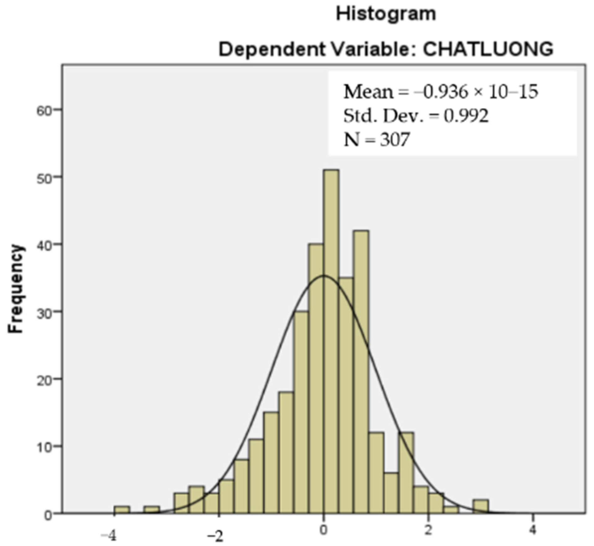
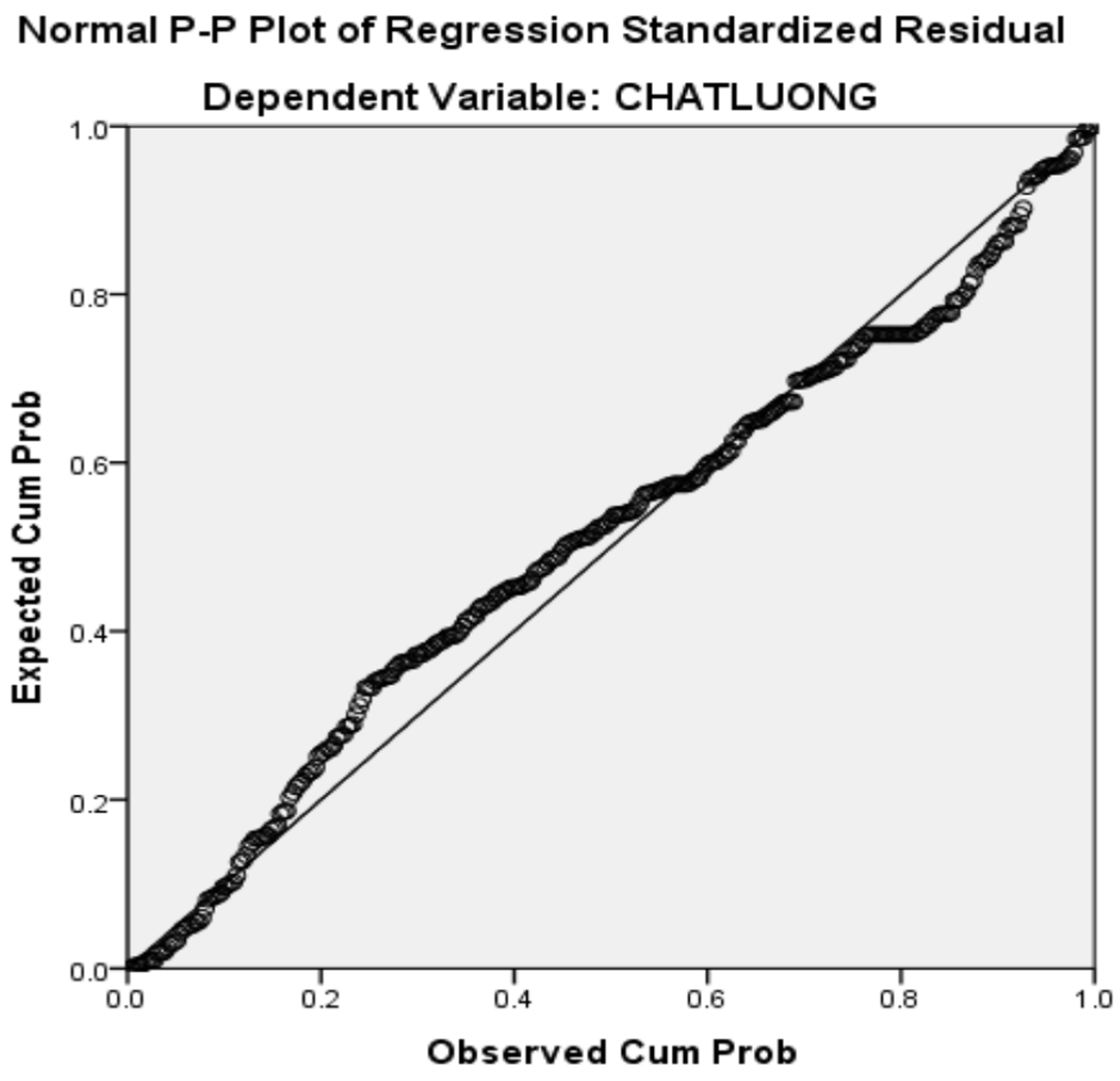
4.1.5. Linear Regression Analysis

Based on the theory and analysis results above, the author included five (5) independent variables of the correction model into the regression analysis, whose results are shown in

Table 9. Model summary.

Model	R	R Square	Adjusted R Square	Std. Error of the Estimate	Durbin-Watson
1	0.644	0.414	0.405	0.43199	1.695

below:

The statistical values for evaluating the fit of the model were R, R², adjusted R², and standard error of the estimate are satisfactory with R² = 41.4 % and adjusted R² as 40.5%. This means the five (5) independent variables included in the model influenced up to 40.5% of the change for the dependent variable, with the remaining 58.6% coming from variables outside the model and from random error. The Durbin–Watson coefficient D = 1.695 shows that the model had no autocorrelation.

The Sig. value of the F-test was 0.000 < 0.05 (

Table 10. ANOVA.

Model		Sum of Squares	df	Mean Square	F	Sig.
1	Regression	39.763	5	7.953	42.615	0.000
	Residual	56.172	301	0.187
	Total	95.935	306

). Thus, the linear regression model was suitable for the population.

Through

Table 11. Linear regression model.

Model		Unstandardized Coefficients		Standardized Coefficients	t	Sig.	Collinearity Statistics
		B	Std. Error	Beta				B
1	(Constant)	0.773	0.229		3.372	0.001
	CUS	0.255	0.072	0.234	3.547	0.000	0.448	2.234
	REL	0.219	0.062	0.222	3.518	0.001	0.489	2.044
	RES	0.195	0.064	0.186	3.074	0.002	0.530	1.888
	INT	0.184	0.064	0.180	2.859	0.005	0.489	2.046
	TAN	−0.066	0.059	−0.065	−1.121	0.263	0.576	1.737

, the following can be seen.

The Sig. value of Tan = 0.263, which is greater than > 0.05, so it was excluded. Thus, the results show that the remaining four variables affect the quality of savings deposit services, namely concern, reliability, responsiveness, and interest rates.

The regression equation is rewritten as follows:

Y = 0.773 + 0.234 × X1 + 0.222 × X2 + 0.186 × X3 + 0.180 × X4

where

Y: Quality of savings deposit service

X1: Customer service

X2: Reliability

X3: Responsiveness

X4: Interest rate

This means:

Provided that the other factors are constant, when the factor of “concern” changes by 1 unit, the quality of savings deposit service will change by 0.234 units.

Provided that the other factors are constant, when the factor of “reliability” changes by 1 unit, the quality of savings deposit service will change by 0.222 units.

Provided that the other factors are constant, when the factor of “responsiveness” changes by 1 unit, the quality of savings deposit service will change by 0.186 units.

Provided that the other factors are constant, when the factor of “interest” changes by 1 unit, the quality of savings deposit service will change 0.18 units.

Assumption of normal distribution of the residuals: The graphs show a normal distribution curve that is superimposed on the histogram (Figure 3). This curve is bell-shaped, which is consistent with the graph of the normal distribution. The mean value is close to 0, and the standard deviation is 0.992, which is close to 1, so we can conclude that the assumption of the normal distribution of the residuals is satisfactory.

In the P–P plot graph, the actual observations are concentrated in a diagonal line close to the expected value diagonal, which means that the residuals have a normal distribution for quality of service and predicted values (Figure 4).

The assumption on a linear relationship and constant variance of the error: The graph of the normalized residuals by the normalized predicted values shows that they are scattered without following any curve. Therefore, this assumption is not violated (Figure 5).

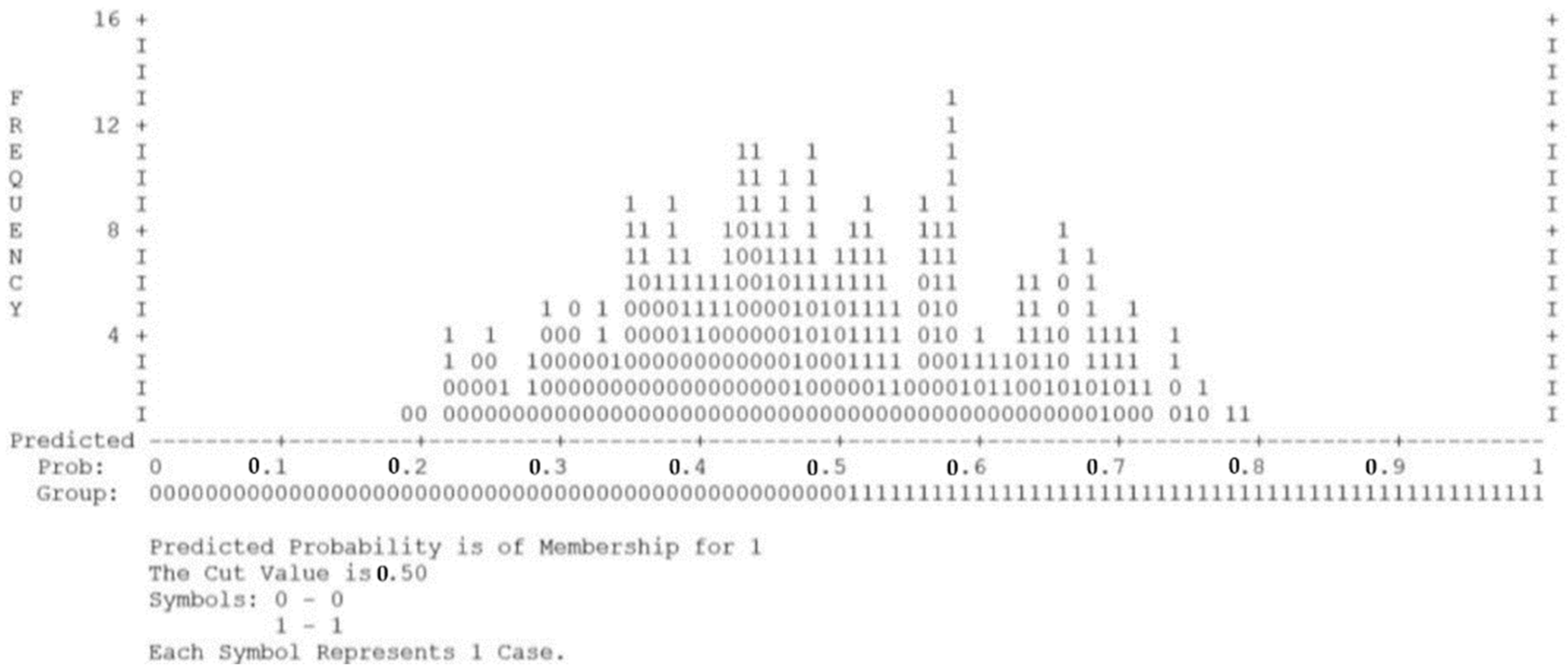
4.2. Results of Binary Logistic Model

In this study, the authors used the Binary Logistic model to calculate the probability of capital withdrawal ahead of time for savings deposits at commercial banks, thereby giving customers advice on appropriate service packages in transactions to avoid the risk of premature capital withdrawal and a very low demand interest rate, greatly affecting customer satisfaction and the service quality of commercial banks. The authors assign to the factor of the probability of capital withdrawal ahead of time 2 values as 0 and 1, where 0 represents the capital non-withdrawal ahead of time and 1 represents capital withdrawal ahead of time. For the probability of capital withdrawal ahead of time, the authors collected data for three (3) independent variables in the model affecting the probability of capital withdrawal ahead of time, including Age (AG): age to present; Education (ED): years of schooling; Monthly income (IN): monthly income in million VND.

The results in

Table 12. Case processing summary.

Unweighted Cases a		N	Percent
Selected Cases	Included in analysis	307	100.0
	Missing cases	0	0.0
	Total	307	100.0
Unselected cases		0	0.0
Total		307	100.0

^a If weight is in effect, see classification table for the total number of cases.

show that the authors collected data from 307 customers who provided complete data and none of them provided missing data.

The results in

Table 13. Omnibus tests of model coefficients.

		Chi-Square	df	Sig.
Step 1	Step	22.807	3	0.000
	Block	22.807	3	0.000
	Model	22.807	3	0.000

show that the Sig. coefficient of all three indexes—step, block, and model—are equal to 0.000 < 0.05 (confidence level of 95%), so the regression model in this study has statistical significance.

The results of

Table 14. Model summary.

Step	−2 Log likelihood	Cox & Snell R Square	Nagelkerke R Square
1	402.235 a	0.072	0.096

^a Estimation terminated at iteration number four because the parameter estimates changed by less than 0.001.

and

Table 15. Classification table ^a.

	Observed		Predicted
			PM		Percentage Correct
			0	1
Step 1	PM	0	111	49	69.4
		1	65	82	55.8
	Overall Percentage				62.9

^a The cut value is 0.500.

show the classification of customers who withdraw capital ahead of time and who do so on schedule based on two criteria—actual observation and prediction. Out of the 160 surveyed customers who had no capital withdrawal ahead of time, 111 customers were predicted to not withdraw capital ahead of time, equivalent to 69.4% of the correct prediction rate. Out of the 147 surveyed customers who withdrew capital on a schedule, the number of customers who were correctly predicted was 82, corresponding to 55.8% of the correct prediction rate.

The results in

Table 16. Variables in the equation.

		B	S.E.	Wald	df	Sig.	Exp(B)
Step 1 a	AG	0.033	0.011	9.526	1	0.002	1.034
	ED	−0.209	0.061	11.742	1	0.001	0.812
	IN	−0.012	0.010	1.346	1	0.246	0.988
	Constant	2.172	0.989	4.825	1	0.028	8.779

^a Variable(s) entered on step 1: AG, ED, and IN.

show that the coefficient Sig_AG = 0.026 < 0.05; Sig_ED = 0.001 < 0.05 (confidence level of 95%) reflects the factors of age and education influence probability of capital withdrawal ahead of time. The coefficient Sig_IN = 0.246 > 0.05 reflects that the factor of income has no impact on the probability of capital withdrawal ahead of time. Based on the results in Table 16, a binary logistic model was constructed, as follows:

$${\log }_e=\left[\frac{{\mathrm{P}}_i}{1-{\mathrm{P}}_i}\right]=2.172+0.033AG-0.209ED$$

The above model reflects that the older the customer, the higher the probability of capital withdrawal on a schedule, which means that before making savings deposits into commercial banks, older customers have thought and considered very carefully this action, so their probability of capital withdrawal on a schedule is very high (observed group predicted probabilities in Figure 6). Furthermore, the low probability of capital withdrawal on schedule from highly educated customers reflects that those with a higher education always consider capital withdrawal when investing in another more profitable field.

Managers of commercial banks need to identify customers who are likely to withdraw capital ahead of time and those who will withdraw capital on schedule in order for the banks and their customers to avoid business risks. Therefore, solutions for advising customers about deposits for appropriate terms, facilitating customers’ deposit savings commending solutions to advise can be recommended. In addition, commercial banks should plan to use the capital in payment management and service supply to integrate a material and financial supply chain for both customers and commercial banks.

4.3. Results and Analysis of the GM (1,1) Model

In this study, using the GM (1,1) model, the actual data from the factor as the number of individual customers in the period of 2017–2020 in a Commercial Bank in Vietnam (CBV) were used to explain the calculation procedure of all other factors in this study (data in the

Table 17. Number of individual customers in 2017–2020.

YEAR	2017	2018	2019	2020
NIS	234,649	270,076	284,260	299,837

). The specific calculation procedure was carried out according to the steps below.

Set up of the original value chain:

$${\mathrm{X}}^{\left(0\right)}=(\mathrm{234,649};\mathrm{270,076};\mathrm{284,260};\mathrm{299,837})$$

Use the cumulative method to calculate the value X⁽¹⁾:

$$\begin{gathered} {\mathrm{x}}_{\left(1\right)}^{\left(1\right)}{=\mathrm{x}}_{\left(1\right)}^{\left(0\right)}=\mathrm{234,649} \\ {\mathrm{x}}_{\left(2\right)}^{\left(1\right)}{=\mathrm{x}}_{\left(1\right)}^{\left(0\right)}{+\mathrm{x}}_{\left(2\right)}^{\left(0\right)}=\mathrm{504,725} \\ {\mathrm{x}}_{\left(3\right)}^{\left(1\right)}{=\mathrm{x}}_{\left(2\right)}^{\left(1\right)}{+\mathrm{x}}_{\left(3\right)}^{\left(0\right)}=\mathrm{788,985} \\ {\mathrm{x}}_{\left(4\right)}^{\left(1\right)}{=\mathrm{x}}_{\left(3\right)}^{\left(1\right)}{+\mathrm{x}}_{\left(4\right)}^{\left(0\right)}=\mathrm{1,088,822} \\ {\mathrm{X}}^{\left(1\right)}=(\mathrm{234,649};\mathrm{504,725};\mathrm{788,985};\mathrm{1,088,822}) \end{gathered}$$

Continue to calculate the average value Ζ⁽¹⁾:

$$\begin{gathered} {\mathrm{z}}_{\left(2\right)}^{\left(1\right)}=0.5\times (\mathrm{234,649}+\mathrm{270,076})=\mathrm{369,687} \\ {\mathrm{z}}_{\left(3\right)}^{\left(1\right)}=0.5\times (\mathrm{270,076}+\mathrm{284,260})=\mathrm{646,855} \\ {\mathrm{z}}_{\left(4\right)}^{\left(1\right)}=0.5\times (\mathrm{284,260}+\mathrm{299,837})=\mathrm{938,903.5} \end{gathered}$$

From the above values, build a system of equations:

$$\{\begin{array}{c}\mathrm{270,076}+\mathrm{a}\times \mathrm{369,687}=\mathrm{b}\\ \mathrm{284,260}+\mathrm{a}\times \mathrm{646,855}=\mathrm{b}\\ \mathrm{299,837}+\mathrm{a}\times \mathrm{938,903.5}=\mathrm{b}\end{array}$$

From the system of equations above, make the matrices and find the values of a and b, as follows:

$$\begin{gathered} \mathrm{B}=\left[\begin{array}{ll}-\mathrm{369,687}& 1\\ -\mathrm{646,855}& 1\\ -\mathrm{938,903.5}& 1\end{array}\right];{\mathrm{Y}}_{\mathrm{n}}=\left[\begin{array}{l}\mathrm{270,076}\\ \mathrm{284,260}\\ \mathrm{299,837}\end{array}\right] \\ \hat{\mathsf{\theta }}=\left[\begin{array}{c}\mathrm{a}\\ \mathrm{b}\end{array}\right]{=(\mathrm{B}}^{\mathrm{T}}{\mathrm{B})}^{-1}{\mathrm{B}}^{\mathrm{T}}{\mathrm{y}}_{\mathrm{N}}=\left[\begin{array}{r}-0.0523\\ \mathrm{250,638.5971}\end{array}\right] \end{gathered}$$

After obtaining the values for coefficients a and b, make a differential equation, as follows:

$$\frac{{\mathrm{dx}}^{(1)}}{\mathrm{dk}}-0.0523\times {\mathrm{x}}^{(1)}=\mathrm{250,638.5971}$$

Set up the forecasting equation:

$${\widehat{\mathrm{X}}}_{(\kappa +1)}^{(1)}=[\mathrm{234,649}-\frac{\mathrm{250,638.5971}}{(-0.0523)}]\times e^{-(-0.0523)\mathsf{\kappa }}+\frac{\mathrm{250,638.5971}}{(-0.0523)}$$

In turn, assign values k = 0, 1, 2, 3, 4, 5, 6, and 7 into the above equation to calculate the predicted values:

$$\begin{array}{l}{\hat{\mathrm{x}}}_{\left(1\right)}^{\left(1\right)}=\mathrm{234,649}\Rightarrow {\hat{\mathrm{x}}}_{\left(1\right)}^{\left(0\right)}={\widehat{x}}_{\left(1\right)}^{\left(1\right)}=\mathrm{234,649}\\ {\widehat{x}}_{\left(2\right)}^{\left(1\right)}=\mathrm{504,553.87}\Rightarrow {\hat{\mathrm{x}}}_{\left(2\right)}^{\left(0\right)}={\hat{\mathrm{x}}}_{\left(2\right)}^{\left(1\right)}-{\hat{\mathrm{x}}}_{\left(1\right)}^{\left(1\right)}=\mathrm{269,904.87}\\ {\widehat{x}}_{\left(3\right)}^{\left(1\right)}=\mathrm{788,948.58}\Rightarrow {\hat{\mathrm{x}}}_{\left(3\right)}^{\left(0\right)}={\hat{\mathrm{x}}}_{\left(3\right)}^{\left(1\right)}-{\hat{\mathrm{x}}}_{\left(2\right)}^{\left(1\right)}=\mathrm{284,394.72}\\ {\widehat{x}}_{\left(4\right)}^{\left(1\right)}=\mathrm{1,088,611.03}\Rightarrow {\hat{\mathrm{x}}}_{\left(4\right)}^{\left(0\right)}={\hat{\mathrm{x}}}_{\left(4\right)}^{\left(1\right)}-{\hat{\mathrm{x}}}_{\left(3\right)}^{\left(1\right)}=\mathrm{299,662.45}\\ {\widehat{x}}_{\left(5\right)}^{\left(1\right)}=\mathrm{1,404,360.87}\Rightarrow {\hat{\mathrm{x}}}_{\left(5\right)}^{\left(0\right)}={\hat{\mathrm{x}}}_{\left(5\right)}^{\left(1\right)}-{\hat{\mathrm{x}}}_{\left(4\right)}^{\left(1\right)}=\mathrm{315,749.84}\\ {\widehat{x}}_{\left(6\right)}^{\left(1\right)}=\mathrm{1,737,061.74}\Rightarrow {\hat{\mathrm{x}}}_{\left(6\right)}^{\left(0\right)}={\hat{\mathrm{x}}}_{\left(6\right)}^{\left(1\right)}-{\hat{\mathrm{x}}}_{\left(5\right)}^{\left(1\right)}=\mathrm{332,700.87}\\ {\widehat{x}}_{\left(7\right)}^{\left(1\right)}=\mathrm{2,087,623.66}\Rightarrow {\hat{\mathrm{x}}}_{\left(7\right)}^{\left(0\right)}={\hat{\mathrm{x}}}_{\left(7\right)}^{\left(1\right)}-{\hat{\mathrm{x}}}_{\left(6\right)}^{\left(1\right)}=\mathrm{350,561.92}\\ {\hat{\mathrm{x}}}_{\left(8\right)}^{\left(1\right)}=\mathrm{2,457,005.51}\Rightarrow {\hat{\mathrm{x}}}_{\left(8\right)}^{\left(0\right)}={\hat{\mathrm{x}}}_{\left(8\right)}^{\left(1\right)}-{\hat{\mathrm{x}}}_{\left(7\right)}^{\left(1\right)}=\mathrm{369,381.85}\end{array}$$

Using the same calculation, the authors obtained the predictions for the criteria in the period of 2021–2024, as shown in

Table 18. Results of forecasting.

YEAR	NIS	NCC	FEP	CBE	NSR	PBT
2021	315,749.84	6536.69	19,780.00	19,039.60	128,997,134.58	678,829.58
2022	332,700.87	7889.57	20,971.11	19,748.94	169,534,757.96	726,120.81
2023	350,561.92	9522.46	22,233.95	20,484.71	222,811,415.55	776,706.61
2024	369,381.85	11,493.29	23,572.83	21,247.88	292,830,375.88	830,816.52

.

After calculating the predicted values, Formula (12) was used to test the accuracy of these results and to obtain the average error for the predicted values of these factors, as follows: MAPE_average = 4.48%. This result showed that the predicted values of CBV’s business in the period of 2021–2024 was very accurate, confirming that managers can fully use the predicted results in this study to plan and build business strategies for CBV from 2021–2024.

The predictions of the factors in this study have important implications for commercial banks when building and planning strategies for preparing resources to meet the needs of customers at the right time, the right place, and the right quality. This prediction result will help managers identify resources that are suitable for facilities, such as equipment, capital, human resources, and space, in order to meet customer needs as the basis to make strategic decisions for determining the appropriate cost for each service package. This result is also a milestone for commercial banks’ business departments to achieve within a certain period, and to direct marketing and other business activities for the fulfillment of the goals in the forecast sheet.

5. Discussion

After the supply of products and services, customer service is one of the most important tasks in sales in order to maintain a long-term attachment with a bank for customers. Mobilization of savings deposits is no exception. On the other hand, good customer service also promotes the image and service quality of the branch to other potential customers in the area. This is especially the case if mistakes occur in the first transactions with customers, making a bad impression. Customers will not be willing to return if it is not necessary. If a bank does not comply with the working time, this will lead to a delay for many of the programs that have been implemented but that do not comply with the regulations.

The system of providing services related to savings deposits in the banks also has many limitations. In particular, more and more criminals are using fake automated teller machine (ATM) cards to withdraw customers’ money from ATM, and there are no sanctions for these events, causing difficulties for both customers and banks, which leads to a lack of customer satisfaction. Managers of commercial banks need to correct and prescribe the specific working time for staff, if necessary, so they can set up a periodic inspection team to ensure that the department in charge is always ready to welcome customers when trading time arrives. Currently, technology plays a very important role in the development of modern banking services, especially in the context of an increasing customer population when commercial banks have limited human resources. Therefore, commercial banks need to promote and direct customers toward e-banking in order to minimize the number of customers coming for deposit savings transactions at the counter, as well as to minimize transactions that need staff involvement. For the fulfillment of this objective, banks need to advertise e-banking services to their customers. Each staff member needs to encourage dedicated advice and guidance so that customers find it easy to access digital technology. In addition, it is necessary to promote the completion of system solutions such as extending bandwidth, transmission lines, and contact suppliers to complete new banking services in order to guarantee smooth and uninterrupted online transactions. In the future, when banks have too much cash, the Vietnamese government needs to consider a policy of gradually lowering the deposit interest rate to 0% and having negative interest rates (deposit fees). This policy has been applied by countries around the world to direct savings and idle cash flows into other investment channels so as to benefit the economy. This affects low lending rates, thereby making it easier for businesses and low-income people to access loan sources to help businesses develop and to ensure social security for low-income people.

6. Conclusions

In this study, three models representing the past, present, and future (Servqual model, the Binary Logistic model, and the Grey forecasting model, respectively) were used. This study evaluates in detail the criteria for models in the field of savings deposit mobilization in commercial banks. The study was conducted with a large sample size (307 customers) and was very successful at using qualitative research in combination with quantitative research. The research results show the factors affecting the satisfaction of customers who make savings deposits at commercial banks, as well as the factors affecting the probability of capital withdrawal ahead of time of savings deposits at commercial banks. It also predicted the number of customers and important criteria for commercial banks from 2021 to 2024. The results of this study show that the factors of customer care, reliability, and responsiveness have a great impact on customer’s satisfaction while using services at commercial banks. Therefore, banks need to ensure and maintain good customer care services to help promote the bank’s brand in the customers’ mind. When customers see good service quality, it will lead to further usage of other services, thereby forming a loyalty from its customers. Moreover, word-of-mouth also plays an important role in attracting the new customers. This helps the bank stabilize its business situation and develop sustainably.

Limitations: The results of this study have important implications for the managers of commercial banks in Vietnam. However, many modern models can be used simultaneously to find more useful solutions. In addition, the results presented here are still limited in terms of time, human resources, and technology. A number of recent studies have described the impact of the Covid-19 pandemic on exchange rates and its effect on the stock market (Lee et al. 2021). These impacts also indirectly affect banking business activities (Zhang et al. 2020). In the future, evaluating this influence on the business situation of commercial banks in Vietnam should be studied. Research should be carried out in combination with environmental factors and regulations and policies of state management in the field of commercial banks in order to achieve better solutions. Research should be carried out in combination with other models and methods to help managers of commercial banks have greater perspectives and multidimensional reference systems, thus contributing to sustainable commercial banking strategies and development.

References

1. Ahmed, Mobin. 2017. Service Quality Measurement regarding Banking Sector. International Journal of Business and Social Science 8: 116–27. [Google Scholar]
2. Al Nageim, Hassan, Ravindra Nagar, and Paulo Lisboa. 2007. Comparison of neural network and binary logistic regression methods in conceptual design of tall steel buildings. Construction Innovation 7: 240–53. [Google Scholar] [CrossRef]
3. Anand, Vijay, and M. Selvaraj. 2013. Evaluation of service quality and its impact on customer satisfaction in Indian banking sector-A comparative study using Servperf. Life Science Journal 10: 3267–74. [Google Scholar]
4. Araveeporn, Autcha. 2021. The Higher-Order of Adaptive Lasso and Elastic Net Methods for Classification on High Dimensional Data. Mathematics 9: 1091. [Google Scholar] [CrossRef]
5. Bente, Corneliu. 2012. Concepts of Service Quality Measurement in Banks. Oradea: University of Oradea, pp. 889–94. [Google Scholar]
6. Chandra, Mahesh, and James P. Neelankavil. 2008. Product development and innovation for developing countries: Potential and challenges. Journal of Management Development 27: 1017–25. [Google Scholar] [CrossRef]
7. Chen, Yuan Chen, Hsien Chueh Peter Yang, Cheng Wu Chen, and Tsung Hao Chen. 2008. Diagnosing and revising logistic regression models: Effect on internal solitary wave propagation. Engineering Computations 25: 121–39. [Google Scholar] [CrossRef]
8. Cristian, Negrutiu, Cristinel Vasiliu, and Calcedonia Enache. 2020. Sustainable Entrepreneurship in the Transport and Retail Supply Chain Sector. Risk Financial Manag 13: 267. [Google Scholar] [CrossRef]
9. De Gaetano, Davide. 2018. Forecast Combinations for Structural Breaks in Volatility: Evidence from BRICS Countries. Journal of Risk Financial Manage 11: 64. [Google Scholar] [CrossRef] [Green Version]
10. Durst, Susanne, and Wolfgang Gerstlberger. 2021. Financing Responsible Small- and Medium-Sized Enterprises: An International Overview of Policies and Support Programmes. Journal Risk Financial Manage 14: 10. [Google Scholar] [CrossRef]
11. Eboli, Laura, and Gabriella Mazzulla. 2009. An ordinal logistic regression model for analysing airport passenger satisfaction. EuroMed Journal of Business 4: 40–57. [Google Scholar] [CrossRef]
12. Financial Report. 2021. Available online: https://www.bidv.com.vn/ (accessed on 5 June 2021).
13. Gerbing, W. David, and James C. Anderson. 1988. An Updated Paradigm for Scale Development Incorporating Unidimensionality and Its Assessment. Journal of Marketing Research 25: 186–92. [Google Scholar] [CrossRef]
14. Hair, F. Joseph, Rolph E. Anderson, Ronald L. Tatham, and William Cormack Black. 1998. Multivariate Data Analysis, 5th ed. Upper Saddle River: Prentice Hall. [Google Scholar]
15. Hair, F. Joseph, William Cormack Black, Barry J. Babin, and Rolph E. Anderson. 2009. Multivariate Data Analysis. Upper Saddle River: Prentice Hall. [Google Scholar]
16. Jabnoun, Naceur, and Hussein A. Hassan Al-Tamimi. 2003. Measuring perceived service quality at UAE commercial banks. International Journal of Quality & Reliability Management 20: 458–72. [Google Scholar] [CrossRef]
17. Kaiser, F. Henry. 1974. An index of factorial simplicity. Psychometrika 39: 31–36. [Google Scholar] [CrossRef]
18. Karimi, Tooraj, and Arvin Hojati. 2020. Designing a medical rule model system by using rough–Grey modeling. Grey Systems: Theory and Application 10: 513–27. [Google Scholar] [CrossRef]
19. Ke, Zhang. 2013. Random simulation method for accuracy test of grey prediction model. Grey Systems: Theory and Application 3: 26–34. [Google Scholar] [CrossRef]
20. Lee, Chi Chuan, Chien Chiang Lee, and Yizhong Wu. 2021. The impact of COVID-19 pandemic on hospitality stock returns in China. International Journal of Finance & Economics, 1–14. [Google Scholar] [CrossRef]
21. Li, Shuliang, Ke Gong, Bo Zeng, Wenhao Zhou, Zhouyi Zhang, Aixing Li, and Zhang Li. 2021. Development of the GM(1,1) model with a trapezoidal possibility function and its application. Grey Systems: Theory and Application. [Google Scholar] [CrossRef]
22. Li, Xiaoning, Xinbo Liao, Xuerui Tan, and Haijing Wang. 2014. Using grey relational analysis to evaluate resource configuration and service ability for hospital on public private partnership model in China. Grey Systems: Theory and Application 4: 260–72. [Google Scholar] [CrossRef]
23. Nguyen, Dinh Tho. 2011. Scientific Research Methods in Business. Hanoi: Social Labor Publication. [Google Scholar]
24. Nguyen, Han Khanh. 2020. Combining DEA and ARIMA Models for Partner Selection in the Supply Chain of Vietnam’s Construction Industry. Mathematics 8: 866. [Google Scholar] [CrossRef]
25. Nguyen, Han Khanh. 2021. Applications Optimal Math Model to Solve Difficult Problems for Businesses Producing and Processing Agricultural Products in Vietnam. Axioms 10: 90. [Google Scholar] [CrossRef]
26. Nunnally, C. Jum, and Ira H. Bernstein. 1994. Psychometric Theory, 3rd ed. New York: McGraw-Hill. [Google Scholar]
27. Oguz, Fatih, and Shimelis Assefa. 2014. Faculty members’ perceptions towards institutional repository at a medium-sized university: Application of a binary logistic regression model. Library Review 63: 189–202. [Google Scholar] [CrossRef]
28. Omondi, Ochieng Peter. 2019. Resource-based theory of college football team competitiveness. International Journal of Organizational Analysis 27: 834–56. [Google Scholar] [CrossRef]
29. Omondi, Ochieng Peter. 2021. Financial performance of the United Kingdom’s national non-profit sport federations: A binary logistic regression approach. Managerial Finance 47: 868–86. [Google Scholar] [CrossRef]
30. Parasuraman, Valarie, Zeithaml Zeithaml, and Leonard Berry. 1985. A Conceptual Model of Service Quality and its Implication for Future Research (SERVQUAL). Journal of Marketing 49: 41–50. [Google Scholar] [CrossRef]
31. Shetty, H. Shilpa, and Theresa Nithila Vincent. 2021. The Role of Board Independence and Ownership Structure in Improving the Efficacy of Corporate Financial Distress Prediction Model: Evidence from India. Journal Risk Financial Manage 14: 333. [Google Scholar] [CrossRef]
32. Silvestro, Rhian, and Paola Lustrato. 2014. Integrating financial and physical supply chains: The role of banks in enabling supply chain integration. International Journal of Operations & Production Management 34: 298–324. [Google Scholar] [CrossRef]
33. Thu, Hoa. 2020. Average Life Expectancy of Vietnam through the Results of the 2019 Population and Housing Census–Issues. Available online: http://consosukien.vn/ (accessed on 5 June 2021).
34. Uddin, Md Rasel, Akash Saha, Md Julfikar Ali, and Md Jewel Rana. 2016. Determinants of Service Quality Factors towards the Public Specialized Banks of Bangladesh, Global Journal of Management and Business Research: A Administration and Management. Global Journals 6: 42–50. [Google Scholar]
35. Wang, Chia Nan, Han Khanh Nguyen, and Ruei Yuan Liao. 2017. Partner Selection in Supply Chain of Vietnam’s Textile and Apparel Industry: The Application of a Hybrid DEA and GM (1,1) Approach. Mathematical Problems in Engineering 2017: 1–16. [Google Scholar] [CrossRef] [Green Version]
36. Wang, Chia Nan, Tien Muoi Le, Han Khanh Nguyen, and Hong Ngoc Nguyen. 2019. Using the Optimization Algorithm to Evaluate the Energetic Industry: A Case Study in Thailand. Processes 7: 87. [Google Scholar] [CrossRef] [Green Version]
37. Wood, H. Emma. 2006. The internal predictors of business performance in small firms: A logistic regression analysis. Journal of Small Business and Enterprise Development 13: 441–53. [Google Scholar] [CrossRef]
38. Xuemei, Li, Yun Cao, Junjie Wang, Yaoguo Dang, and Yin Kedong. 2019. A summary of grey forecasting and relational models and its applications in marine economics and management. Marine Economics and Management 2: 87–113. [Google Scholar] [CrossRef]
39. Zhang, Dayong, Min Hua, and Qiang Ji. 2020. Financial markets under the global pandemic of COVID-19. Finance Research Letters 36: 101528. [Google Scholar] [CrossRef] [PubMed]
Figure 1. Physical and financial supply chain in banks (Silvestro and Lustrato 2014).
Jrfm 14 00357 g001
Figure 2. Research process.
Jrfm 14 00357 g002
Figure 3. Regression standardized residual.
Jrfm 14 00357 g003
Figure 4. Normal P–P plot of regression standardized residual.
Jrfm 14 00357 g004
Figure 5. Regression standardized predicted value.
Jrfm 14 00357 g005
Figure 6. Observed groups’ predicted probabilities.
Jrfm 14 00357 g006