4.1. Efficiency of Factor Allocation
The quantities
and
are measuring the aggregate real income and the aggregated real consumption per period of the whole society. We consider these two variables to discuss the difference in the outcomes between our approach and the approach of
Laitner (
1982).
Laitner (
1982) focused on these variables and showed that the derivatives of
and
with respect to the number of firms in the oligopolistic market are strictly positive. However, these outcomes do not hold necessarily if the firm owners are members of the young generation.
We are interested in changes of the steady-state equilibrium. Particularly, we want to know how the relevant variables will change, if the number of firms in the oligopolistic sector will increase. In other words, we are interested in the changes induced when the competition in the oligopolistic sector is becoming tougher. Therefore, the most important aspect is the change of the capital intensity, given by the following:
The numerator of (49) is obviously positive, and the denominator is negative because of the stability condition (42). From this, we can derive the following proposition.
Proposition 1. In a two-sector model with an imperfect competitive market, an increase of an oligopolistic market’s number of firms leads to a decline of the steady-state capital stock and capital intensity, given the local stability of the steady-state equilibrium.
This means that the steady-state capital intensity is declining if the number of firms is increasing. The reason for this outcome is that the effect that the income of the young generation, which consists of wage and profit incomes, will decline if the number of firms increases in the oligopolistic sector. Decisive for this result is that the profit share of the firms will decline, while the income shares of the capital owner and wage earners will increase, if the number of firms increases. Because of this consideration, the income share received by the young generation will also decline. Consequently, the steady-state capital stock will decline if the competition in the oligopolistic sector becomes tougher. This result is the opposite of the result derived by
Laitner (
1982). In his model, the old generation owns the firms, and if the profit share declines, the income share of the young working generation increases, and, additionally, they will invest less of their savings in firm shares and more in physical capital, even if the interest rate declines. As a consequence, a tougher competition in the oligopolistic sector increases the steady-state capital stock.
To get a deeper understanding, we consider the change of the ratio between the quantities produced in the oligopolistic and competitive sector. In the steady-state equilibrium, the ratio,
, can be written as follows:
Differentiating (43) with respect to the number of firms delivers the following:
Proposition 2. If the number of firms in the oligopolistic sector increases, the production will shift from the competitive to the oligopolistic sector.
This result is as expected, because the price of the good produced in the oligopolistic sector decreases with an increasing number of firms. Therefore, the relative price of the good produced in the competitive sector is becoming more expensive, so that relatively less of these goods are demanded, while the relative demand for the goods in the oligopolistic sector increases.
However, this does not necessarily mean that the output of the oligopolistic sector will increase if the competition in this sector becomes tougher. To show what will happen with the steady-state outputs of both sectors, we differentiate Equations (25) and (26):
As in
Laitner (
1982), the changes of the quantities of the competitive and oligopolistic sector can be split up into a static and a dynamic effect. The first summand in (51) and (52) represents the static effect, which is caused by the increasing competition in the oligopolistic sector and which indicates the change of the allocation of input factors. This results in a reallocation of input factors from the competitive to the oligopolistic sector, and thus leads to an increase of the output in the latter sector and to a decline of the output of the former sector. In other words, the reallocation of input factors takes place because the increasing competition reduces the distortions caused by the oligopolistic market structure. The increasing competition leads to a decline of the price of the goods produced in the oligopolistic sector, which increases the relative price of the goods produced in the competitive sector, so that the demand for goods in the oligopolistic sector will increase and the demand for goods produced in the competitive sector will decrease.
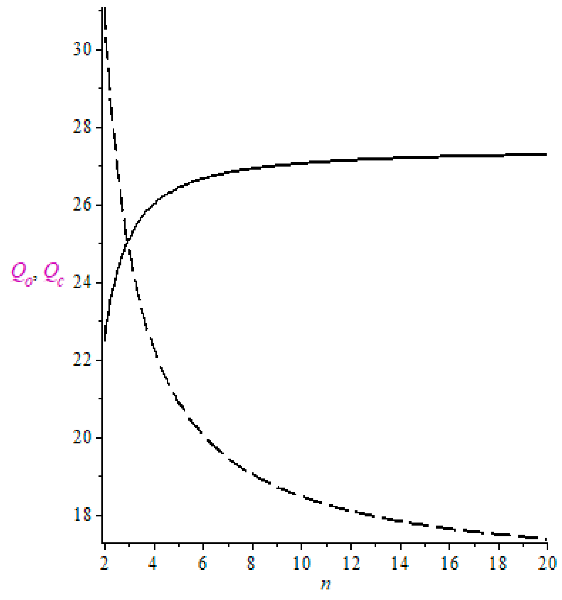
The second summand in (51) and (52) represents a dynamic effect, which is caused by the decline of the capital stock in the long run. This effect leads to a reduction of output in both sectors. While the overall effect regarding the quantity of goods produced in the competitive is uniquely negative, the overall effect on the quantity of goods produced in the oligopolistic sector is ambiguous. To illustrate this, we have calibrated the outcomes for the case of a log-linear utility function and a Cobb–Douglas production function (see
Figure 1,
Figure 2 and
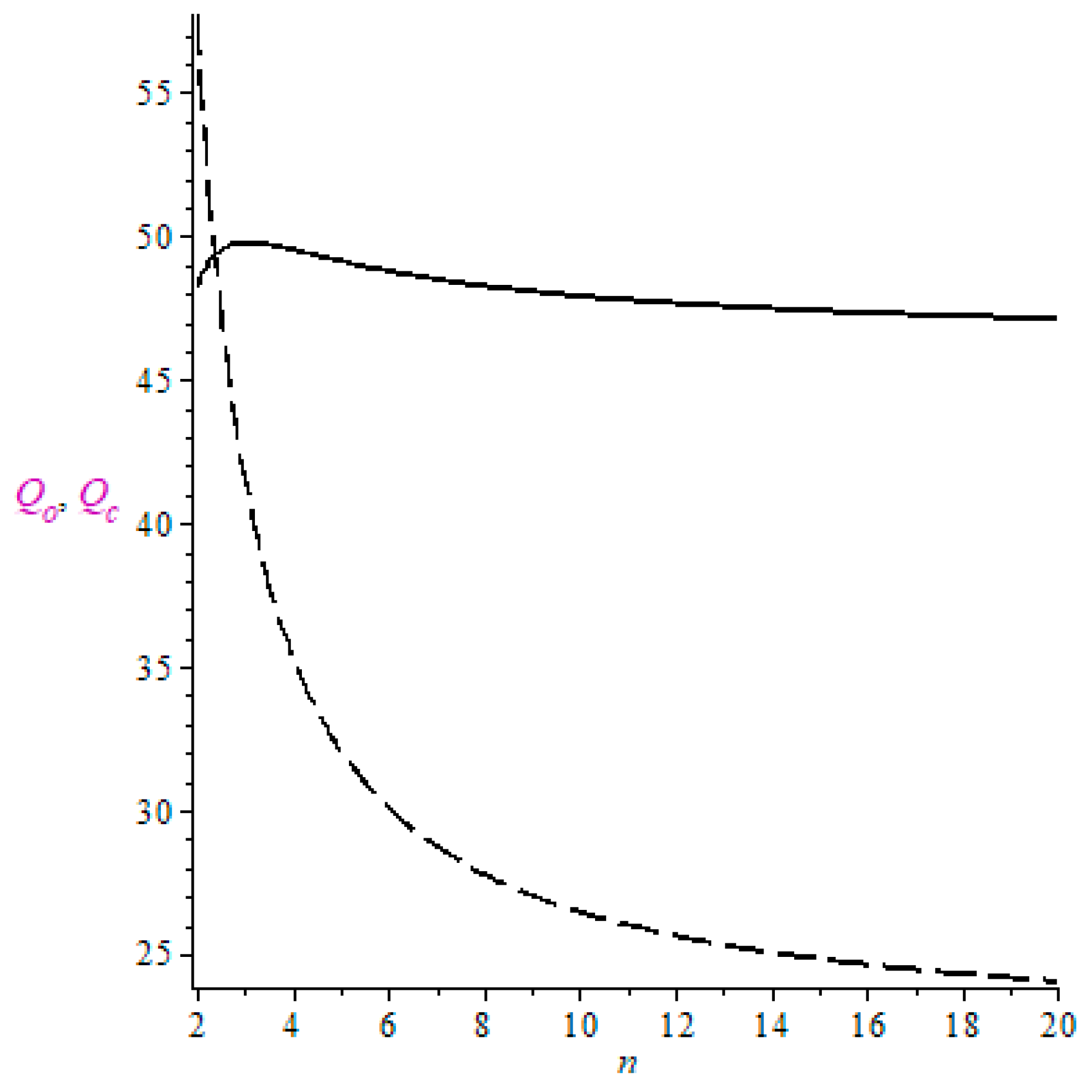
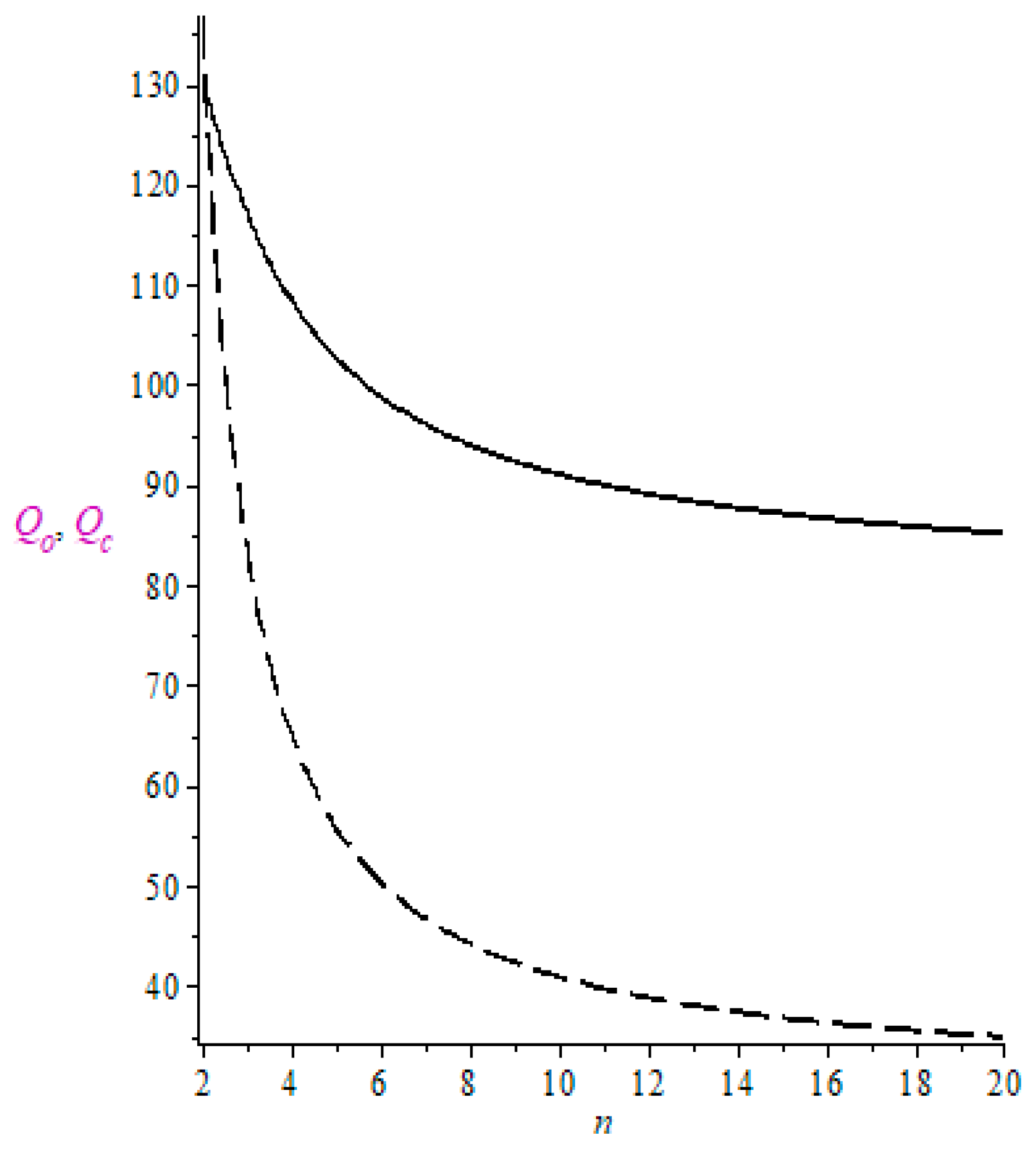
Figure 3).
In all figures, the solid line represents the steady-state equilibrium output of the oligopolistic sector, while the dashed line represents the steady-state output of the competitive sector. To calibrate the three figures, we only changed the value of
, which represents the production elasticity of capital. If the elasticity is sufficiently low, the output of the oligopolistic sector increases, as in
Figure 2, if the elasticity is sufficiently high, the output always declines with an increasing number of competitors, as in
Figure 3; and within certain range of the elasticity coefficients, the output increases with
n and then reaches a maximum, and thereafter the output declines.
Proposition 3. An increase of the number of firms in the competitive sector leads to a decline of the steady-state output of the competitive sector and to an ambiguous change of output produced in the oligopolistic sector.
As noted above, the real income is represented by the quantity of the compounded real consumption good, Q.
Proposition 4. If the competition in the oligopolistic sector becomes tougher, the reaction of the real income is ambiguous.
Proof of Proposition 4. Differentiation of Equation (45) with respect to the number of firms leads to the following result:
where the sign of the expression
. □
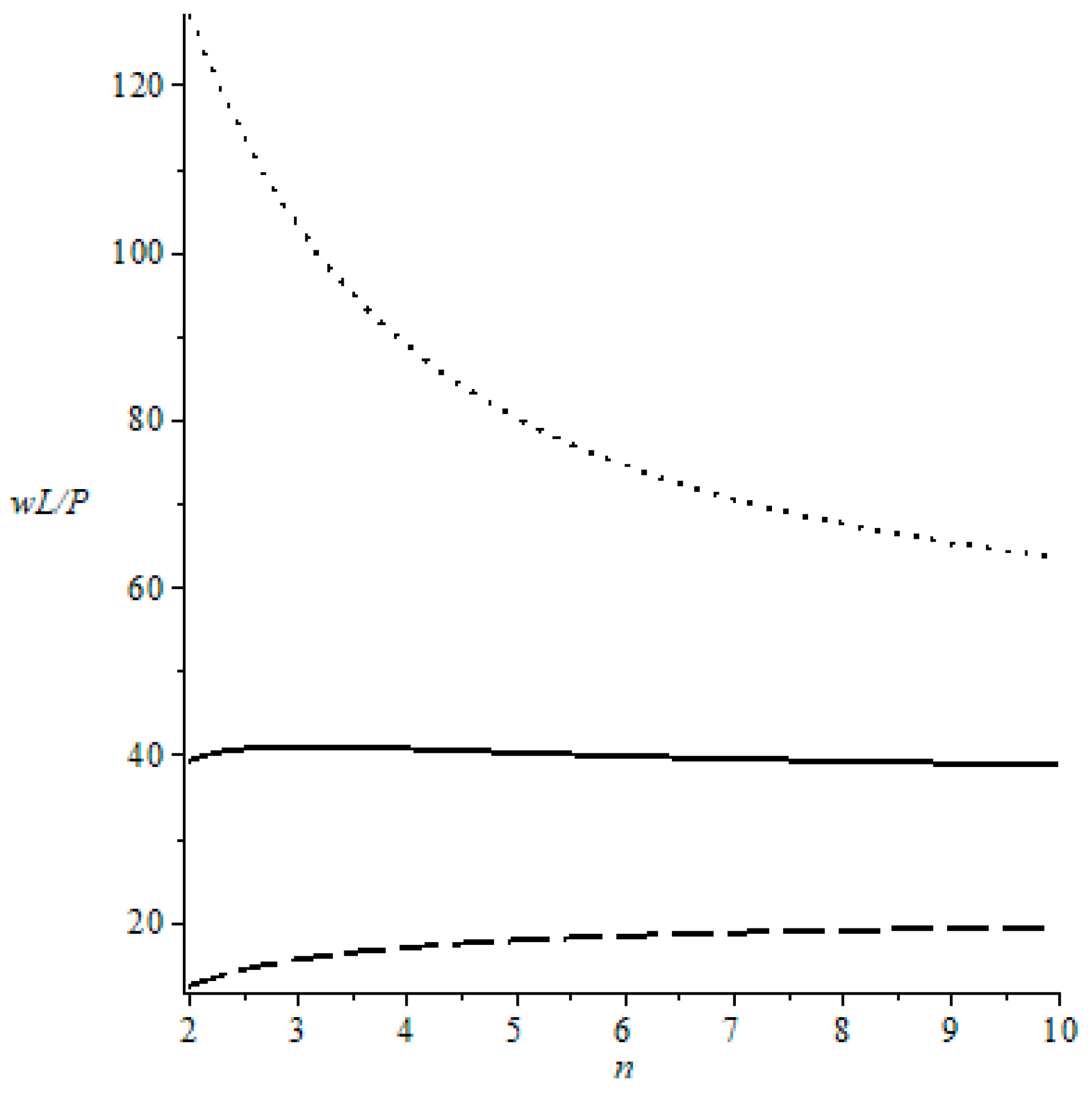
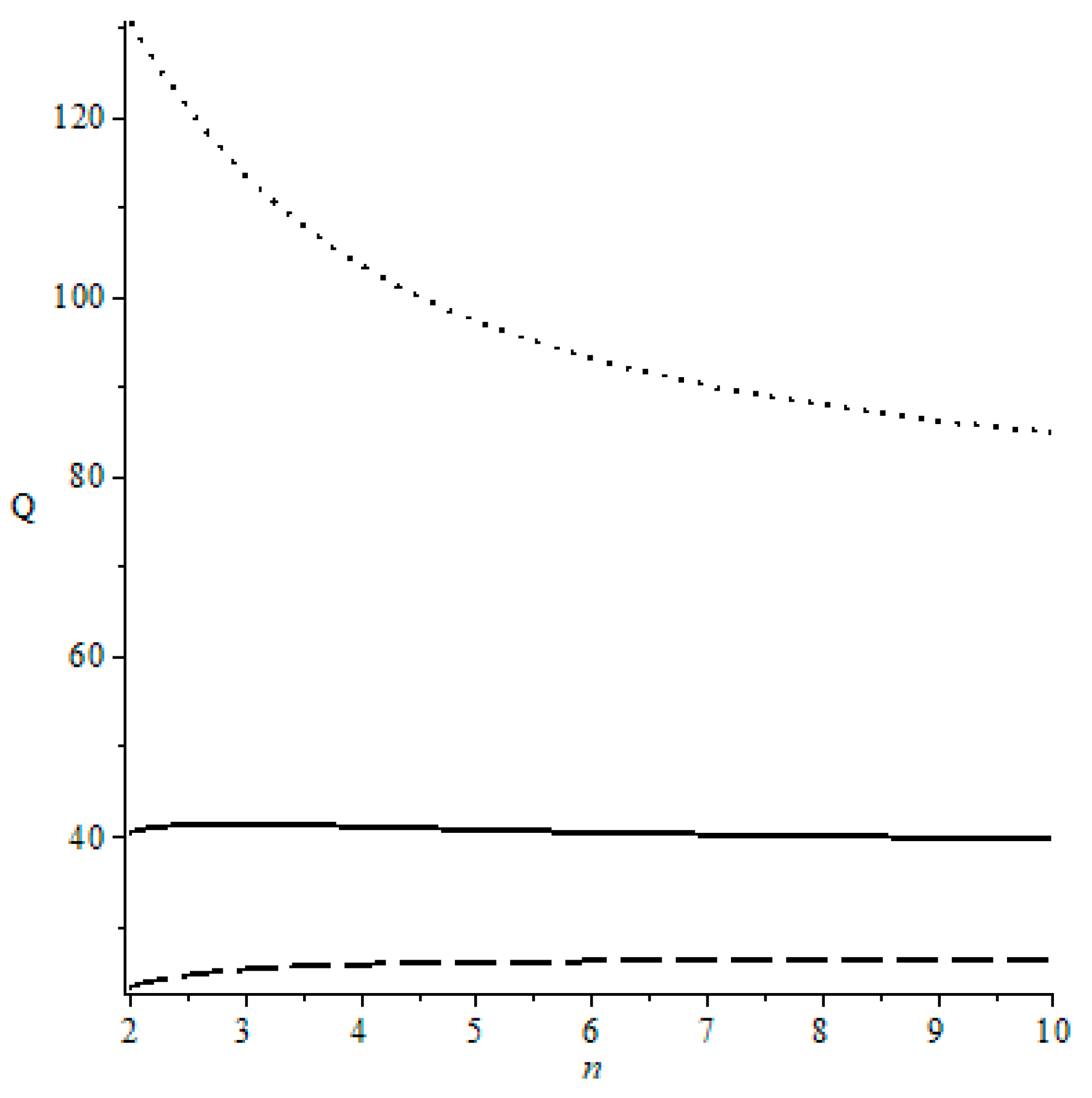
Again, the reaction consists of a static or short-run effect, which leads to an increase of output because of a more efficient input factor allocation. This increase of output is caused by the price change of the good produced in the oligopolistic sector, and a long-run effect, which is negative, is caused by the smaller capital stock. Thus, an increase of the degree of competition in the oligopolistic sector may lead to a decline of real income and consumer surplus in the long run. To illustrate this, we have calibrated Equation (45) along with the number of firms in the oligopolistic sector in
Figure 4.
Unlike the results of
Laitner (
1982), in our model, it is possible that the real income per period will decrease.
Figure 4 presents three different scenarios based on production elasticity of capital. If the elasticity is sufficiently low, then the real income or the quantity of compound goods,
Q, will increase with an increasing numbers of firms (
n) in the oligopolistic sector. If the elasticity is sufficiently high, the opposite happens—the steady-state quantity of
Q will decline with an increasing number of firms in the oligopolistic sector. It also can happen that the quantity of compounded goods will first increase with an increasing number of firms and then it will decrease. However, in our model, it is no longer clear if tougher competition will lead to an increased welfare in terms of real income or consumer surplus.
Proposition 5. If competition increases in the oligopolistic sector, it is in general ambiguous if an increase of the number of firms will lead to an increase or decline of real income or consumer surplus.
The reason for this outcome is that the increase of number of firms changes the inter-generational income distribution, and this change may lead to the fact that the income of the young generation declines sufficiently strongly that the reduction of income, followed by a reduction of savings, cannot be compensated by the increase of production caused the static efficiency gain.
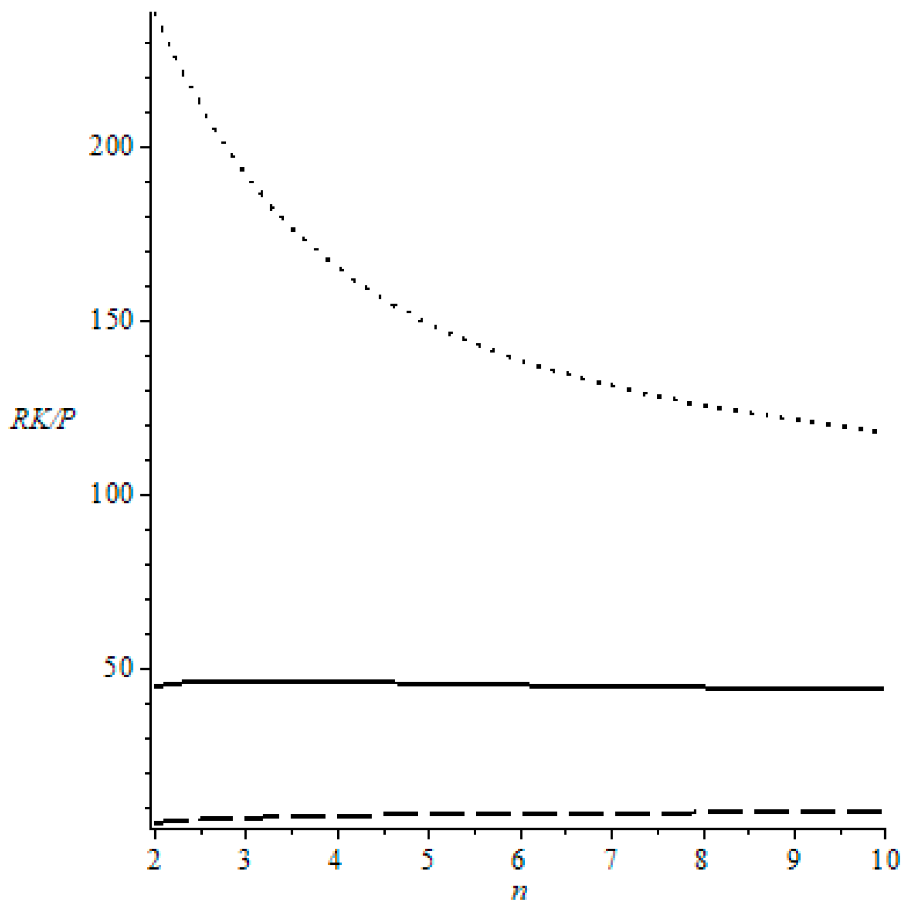
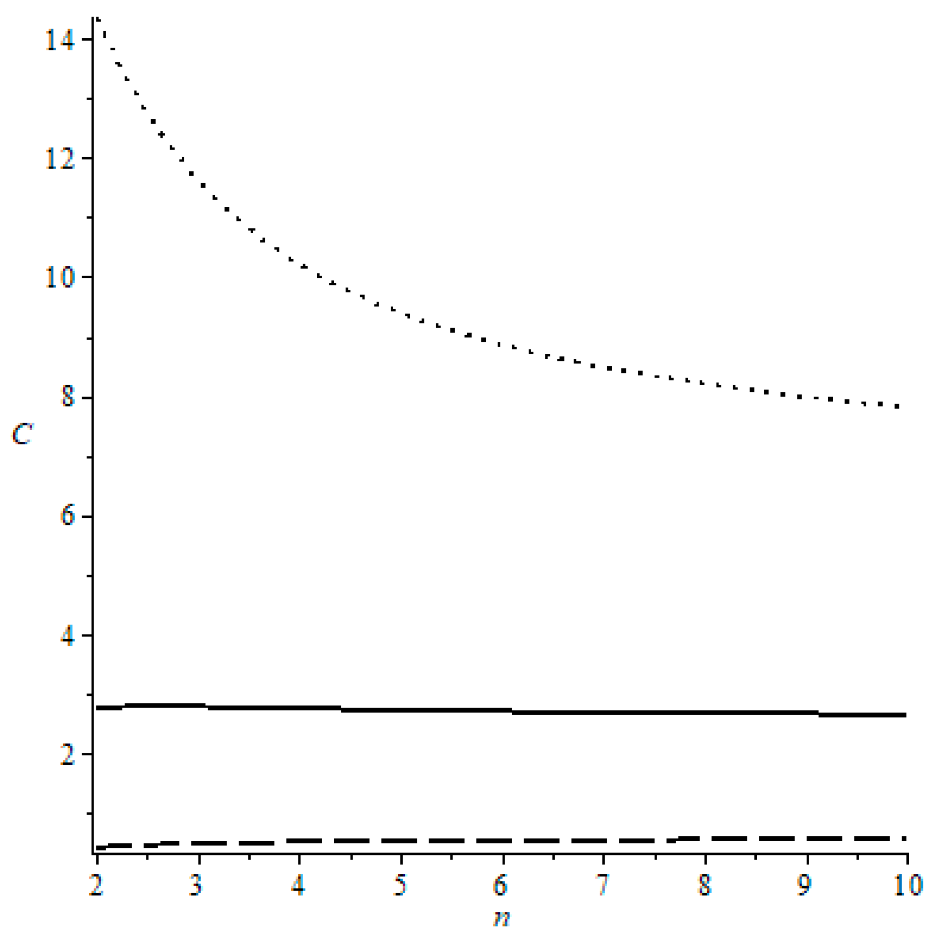
Next, we consider how the aggregate consumption is affected by an increasing number of firms. We differentiate Equation (47) with respect to the numbers of firms in the oligopolistic sector. This gives the following:
The effect on the real consumption is similar to the aggregated quantity of compound goods. Again, the static component of short-run effect has a positive impact, while the dynamic effect on the capital accumulation has a negative impact on the aggregate consumption. We also illustrate this in
Figure 5.
As shown above, regarding the real income, we have only varied the production elasticity of capital. If the elasticity is sufficiently low, the aggregate consumption will increase with an increasing number of firms in the oligopolistic sector; if the elasticity is sufficiently high, the aggregate consumption will decline; and if the elasticity is within certain range (neither too higher nor too low), the consumption has an inverted U-shape form. However, as noted above, these partly surprising results are an outcome of change of the inter-generational income distribution.
4.2. Functional and Inter-Generational Income Distribution
We begin with the nominal national income in terms of the product produced in the competitive sector. The nominal wage incomes are given by the following:
The aggregated nominal capital incomes,
, are as follows:
and the nominal aggregated profits,
, are given by the following:
If we aggregate these incomes, the nominal national income,
, becomes the following:
The nominal national income is equal to the value of goods produced in both sectors, which are measured in terms of the good of the competitive market. The national income measured in terms of the compound good or in purchasing power is given by
. We define the price level,
, in this economy as follows:
Proposition 6. The steady-state price leveldepends negatively on the number of firms in the oligopolistic sector.
The price level declines with the number of firms in the oligopolistic sector. Intuitively, this outcome is obvious, because the tougher the competition in the oligopolistic sector the lower is the price of the good produced in the oligopolistic sector and this reduces the price level.
Now we can calculate the income shares by dividing the labor incomes, the capital incomes and the profit incomes by
. Then we get for the labor share (
), the capital share (
) and the profit share (
) as follows:
and
As can be observed, the relationship between the income shares and the number of firms in the oligopolistic sector is determined by the term
. In
Appendix A, we show that
.
Moreover, the following is clear:
We can summarize these outcomes in the following proposition:
Proposition 7. An increase of the number of firms in the oligopolistic sector will lead to an increase of the labor income share and the capital income share and to a decline of the profit share.
Because of the fact that the income of the firm owners, who receive a wage income and a profit income, exceeds the income of the workers, who only receive a wage income, we can directly conclude that the income distribution of the working generation will become fairer, if the number of firms in the oligopolistic sector increases. Therefore, the incomes of the old generation will also be more equally distributed.
Accordingly, the real labor incomes, real capital incomes and real profit incomes are given by the following:
Finally, we can differentiate the real incomes with respect to the number of firms in the oligopolistic sector to investigate how the different income groups are affected by an increase of the number of firms (competition) in the oligopolistic sector.
An increase of the number of firms in the oligopolistic sector affects the incomes of capital owners, who represent the old generation and the incomes of the workers, who are members of the young generation in a similar way. The income shares will increase, and the reaction of the real income is ambiguous, because both the total production and price will decline. Hence, it is unclear if the real incomes of these two groups will rise or decline. To illustrate these outcomes, we have calibrated the outcomes (see
Figure 6 and
Figure 7).
Proposition 8. If the number of firms in the oligopolistic sector increases, the reaction of the real capital and real labor incomes are ambiguous.
The reaction of the capital and labor incomes depend on two effects. On the one hand, the real income may decline because of the fact that the negative capital accumulation effect outperforms the positive effect generated by the improved production factor allocation, and on the other hand, the income share of workers and capital owners will increase, if the number of firms increases. If the negative capital accumulation effect is, in absolute terms, weaker than the efficiency effect, then the real incomes of workers and capital owners will increase with an increasing number of firms.


