Combining Investment and Tax Strategies for Optimizing Lifetime Solvency under Uncertain Returns and Mortality

Abstract

This paper considers investors who are looking to maximize their probability of remaining solvent throughout their lifetime by using an algorithm that aims to optimize their investment allocation strategy and optimize their tax strategy for withdrawal allocations between tax deferred accounts (TDAs), Roth accounts, and taxable stock and bond accounts. This optimization works with stochastic investment returns and stochastic mortality, extending and combining different investment and tax-efficiency paradigms. We find that optimizing the investment strategy has a much larger impact on the investor remaining solvent than optimizing the tax strategy. This result is key to effectively optimizing both strategies simultaneously. This optimized investment strategy soundly beats a standard target date fund strategy, and the novel optimized tax strategy displays optimal desired properties suggested by non-stochastic tax optimization research.

1. Introduction

This paper offers four main contributions for long-term retirement planning, with a goal to maximize the likelihood of solvency during the lifetime of the investor: (i) The model in the paper combines dynamic portfolio optimization (Merton 1969, 1971; Browne 1995; Dammon et al. 2004; Horan 2006a, 2006b; Das et al. 2019; Jaconetti and Bruno 2008; Spitzer and Singh 2006; Wang et al. 2011) and tax optimization over multiple retirement (and possibly non-retirement) accounts (Brown et al. 2017; Cook et al. 2015; Sumutka et al. 2012; DiLellio and Ostrov 2017, 2018) into one algorithm, whereas these have been handled as separate problems in the literature. (ii) Unlike most tax optimization papers, we include the effect of annual stochastic stock returns, as opposed to using fixed returns. (iii) We also consider optimization that takes into account mortality risk and its concomitant uncertain portfolio horizon, which is more realistic and useful than assuming a known terminal date or looking to optimize portfolio longevity. (iv) The analyses in the paper determine that portfolio optimization has first-order consequences on lifetime portfolio solvency, whereas the impact of tax optimization has second-order consequences. This insight means algorithms may ignore all but the most important features of the tax code when they are considering how to optimize lifetime solvency, making the optimization algorithm computationally feasible. The less important features of the tax code can then be considered independently for each individual and their specific circumstances. Some of the additional results in the paper show that this paper’s approach clearly outperforms a target date fund strategy, that it can determine the optimal time to initiate the collection of social security, and that it can determine whether or not any given annuity should be purchased by an investor. The algorithm also accommodates required minimum distributions (RMDs), infusions to the various accounts, and how to exploit conversions between retirement accounts. The approach shown here extends the academic literature and offers a comprehensive algorithm for practical retirement planning.

The innovations in this approach are timely. Over the coming decades, the United States will see a considerable increase in the percent of its population that is retired. For this coming generation of retirees, there has been a strong shift away from defined benefit plans like pensions in favor of tax deferred accounts (TDAs), such as traditional 401(k)s and IRAs, and Roth accounts (see, for example, Department of Labor (2019), Table E7). In general, the move away from pensions has led to fewer saved resources for these retirees, but more flexibility in how these resources may be used.

This means that many individuals in the coming wave of retirees will need to be more careful and clever than their predecessors if they hope to remain solvent throughout their retirement, but these individuals will also have more tools at their command than previous generations. In particular, to help attain the goal of staying solvent, investors will have the ability to change the investments in their portfolio and to determine how to allocate withdrawals between three types of accounts (TDAs, Roth accounts, and taxable accounts) in order to meet annual consumption needs while adhering to the different tax regulations governing these accounts.

There are key differences in the main features of how a TDA, a Roth account, and a taxable account are taxed in the current American tax system. For TDAs, contributions, in the year they are made, are deductible from taxable income, but withdrawals, in the year they are made, are taxed as income. For Roth accounts, the opposite holds in the sense that contributions are not deductible from taxable income, so they are taxed as income in the year they are made, but then the Roth account is not subject to tax after that. For both TDAs and Roth accounts, we assume that withdrawals are not made before an investor is 59.5 years old, since those withdrawals may be subject to penalties. Starting at age 72, TDAs (though not Roth accounts) are subject to required minimum distributions (RMDs) to avoid penalties. In taxable accounts, bonds and cash are subject to different rules than stock. The interest from cash and bonds is taxed as income. There is no tax on stock, except when it is sold, at which point the stock’s gains are subject to capital gains taxes.

Sources that are taxed as income, such as TDA withdrawals, bond and cash interest, as well as earned income from work, are subject to a progressive tax system with rates ranging from 10% to 37%. Long term capital gains (for stock sold more than a year after being purchased, as we will always assume) are subject to a progressive tax system with rates that are 0%, 15%, or 20%, depending on both income and gains. Wealthier investors may also be subject to a 3.8% Net Investment Income Tax. There are complicated rules to determine what portion of Social Security payments are taxed as income. This paper incorporates those Social Security rules, and the current rules for all the features described above for TDAs, Roth accounts, taxable accounts, and earned income. Since it is unclear how legislation might change the tax structure in the future, we assume the current tax structure holds throughout our calculations in this paper, although we can also incorporate stochastic models for evolving tax structures, as discussed at the end of this paper in the conclusions section.

Determining the optimal investment strategy and determining the optimal tax strategy for allocating withdrawals involve different, complex issues. In part because of this, these two strategic questions are generally separated from each other in the literature, which will be discussed in the next two sections. In one branch of the literature, the optimal investment strategy is explored, but usually the portfolio is considered to be tax free, or, on occasion, the entire portfolio is a taxable account. In the other branch, tax optimization via withdrawal allocations between accounts is considered, but significant assumptions about the investments are made, such as a projected, generally constant, rate of return. The tax code, by necessity, is also simplified, but how much impact do these simplifying assumptions create?

In this paper, we consider both investment optimization and tax optimization1 together, using ideas from both branches of the literature. Instead of the two creating a more complicated optimization when they are combined, we find that they lead to important simplifications instead.

The approach to optimally attaining the investor’s goal of staying solvent will start with determining investment optimization on a post-tax basis using dynamic programming. This computes the optimal dynamic investment portfolio strategy by working chronologically backwards in time. We note that in addition to using the stochastic nature of the investments, we also account for the stochastic nature of mortality, which is uncommon in the literature. However, working with the mortality distribution is crucial for optimizing the probability that the investor will remain solvent until their death. We will compare this to the far more common, but far less realistic, assumption of a projected date of death for the investor. In addition, note that the model is superior to the typical approach of looking to optimize portfolio longevity, since, for example, a 100-year-old investor with significant money should be in a conservative portfolio for their remaining years, not an aggressive one in the hopes of having it last another 100 or more years.

Having obtained the optimal investment strategy, the algorithm optimizes the tax strategy using Monte Carlo simulation, which works chronologically forwards in time. We determine annual taxes by carefully following the progressive taxation rules in America for the two main sources of tax revenue from individuals: Income taxes, which includes tax generated by Social Security income, and capital gains taxes. Within this framework, we look to optimize two variables numerically. The first variable is the level of TDA consumption, which is the key scalar quantity for tax optimization when withdrawal allocations are structured correctly. The theory for this structure is a generalization, and improvement, on what is known as the “informed strategy” in the literature. The second variable is a correction factor that accounts for the fact that we must approximate the portfolio’s overall post-tax worth by using the current pre-tax worth of the three accounts (TDA, Roth, and taxable), and we cannot be certain how much tax will be levied on future withdrawals in the TDA and future realized capital gains in the taxable account.

We find the following key result: The probability that the investor remains solvent is strongly affected by their investment strategy, but the effect of the taxation optimization, while present, is much weaker. For example, for the three investors analyzed in this paper, we will see that investment optimization increases their solvency probability by 16.5, 16.6, and 4.7 percentage points over a standard target date fund strategy, whereas tax optimization increases their solvency probability by, at most, 1.7, 1.2, and 2.8 percentage points respectively. This suggests that adding further complicated details of the tax code or the withdrawal allocation structure between accounts is not worthwhile, as it will not have a meaningful effect on the solvency probability.

This is not to say that tax optimization is not important, of course. Investment optimization may have a far larger effect on the probability of solvency, but tax optimization generates far more stable sources of additional money. So, for example, an investor may have consumption needs of $80,000 every year, while tax optimization may generate an extra $50,000 over the course of retirement. The ability to fund an extra 5/8 of a year will not have much of an effect on their probability of remaining solvent until their death, but no wealth manager should leave an extra $50,000 in tax savings on the table.

In this paper we assume we know the following information about investors: Their current age, the current amount of money in their TDA and Roth accounts, and, for their taxable account, the current amount in bonds (and cash), as well as the current amount in stock and its cost basis. We also assume we are given projections which can vary over time for: (1) the time they will retire and, prior to that, the amount of money they would like to contribute to their TDA and the amount to their Roth in each year they are working, (2) the amount of earned income they will receive each year, (3) standard or itemized deductions for income tax each year, (4) the amount of Social Security income for each year, (5) additional after-tax income each year that is neither earned nor derived from the investor’s three accounts, such as projected inheritance money, for example, (6) the investor’s mortality table, and (7) perhaps most importantly, projected after-tax consumption needs each year, which, if desired, can also be made to depend on the investor’s wealth since investors with less wealth may wish to reduce their consumption and investors with more wealth may wish to increase their consumption. We also assume an annual rate of inflation, the interest rate for the bonds/cash, and the expected return and the covariance matrix for the stochastic stock investments. Since these projections and circumstances will change over time for investors, the algorithm we describe in this paper should be periodically rerun to incorporate any updated information.

A summary of the main contributions of this paper is as follows: (1) The paper develops an approach where dynamic programming for investment optimization can be combined with numerical methods for tax optimization. (2) The optimization approach for the combined investment and tax strategy is extended to the context where both investment returns and mortality are stochastic. (3) The implementation here expands and improves previous tax efficiency approaches, obtaining a simple, but effective, approach to tax optimization. (4) Our results show that investment optimization is far more important than tax optimization for maximizing the probability that an investor can remain solvent. This means that more complicated taxation models with more variables are unlikely to generate meaningful and improved results for a retiree’s solvency probability. (5) The new investment optimization approach in this paper leads to a much higher solvency probability than using a target date fund or a static portfolio if the likelihood of an investor’s death is determined by a mortality table. Furthermore, these advantages become even stronger if the mortality table is replaced with the more common, though unrealistic, assumption of a projected date of death for the investor. (6) The combined optimization algorithm in this paper can be used to determine (a) when an investor should optimally start collecting Social Security, (b) the price at which an annuity transitions from increasing to decreasing the investor’s solvency probability, and (c) how changes in the investors’ saving or spending behavior over time will affect their optimal probability of solvency.

The rest of the paper proceeds as follows. Section 2 briefly relates the new approach shown here to the investment optimization literature, while Section 3 compares this paper’s approach with extant methods in the tax optimization literature. Our model and its assumptions are presented in Section 4. Section 5 contains extensive numerical analyses showcasing the main results in the paper. Discussion and conclusions are in Section 6.

2. Investment Optimization: Past Approaches and Our Approach

Since the optimal choice for investments in a portfolio at any given time depends on considering all potential future investment choices, the optimal choice must be computed by working backwards chronologically. A classic example of this is in Merton (1969) and Merton (1971), which optimized the expected utility of an investor’s terminal wealth by dynamically altering the investor’s fraction of wealth in stocks versus bonds. Merton determined this evolving optimal fraction by solving a Hamilton–Jacobi–Bellman partial differential equation that evolved backwards in time. This was later expanded in a series of papers, Browne (1995), Browne (1997), and Browne (1999), to optimally obtain a goal. Applying dynamic programming instead of partial differential equation methods, Das et al. (2019) showed how to quickly determine the dynamic investment strategy that optimizes the probability of achieving a goal, even when the investor has projected infusions or withdrawals at future times.

In the above literature, the portfolio either had a fixed time horizon or was intended to generate money indefinitely. Since our goal is to optimize the probability of staying solvent throughout an investor’s lifetime, our portfolio horizon is neither fixed nor infinite. It is stochastic, with a probability distribution defined by the appropriate mortality table for the investor.

The above literature assumes the investor’s portfolio is not subject to taxes. Dammon et al. (2004) shows how to optimize utility in a taxable stock portfolio, subject to capital gains being determined by the average cost basis method. By using the average cost basis method, their state space must accommodate three variables: Time, wealth, and the amount of money in the basis. Attempting to expand this method to our situation would require six state space variables: Time, wealth in the TDA, wealth in the Roth, wealth in the taxable bond account, wealth in the taxable stock account, and amount of money in the taxable stock basis. The so-called “curse of dimensionality” makes this approach with six state variables computationally infeasible.

We therefore must use a different approach involving approximations: We treat the three accounts as a combined portfolio, using just two state space variables, time and the post-tax worth of the combined portfolio. This means we generate a single optimal investment strategy for the entire portfolio. This can be accomplished by either applying this optimal investment strategy to each of the three accounts or, if desired, by using different investments in the three accounts in a manner that combines into the desired optimal investment allocations. This latter approach can be used to minimize taxes by, for example, shifting more bonds into the TDA which shields investors from annual taxes on interest that they would be subject to in a taxable account. While this should be done because it will typically benefit investors, it is also a minor effect, so for our calculations we use the same investment allocation in all three accounts.

3. Tax Optimization: Past Approaches and Our Approach

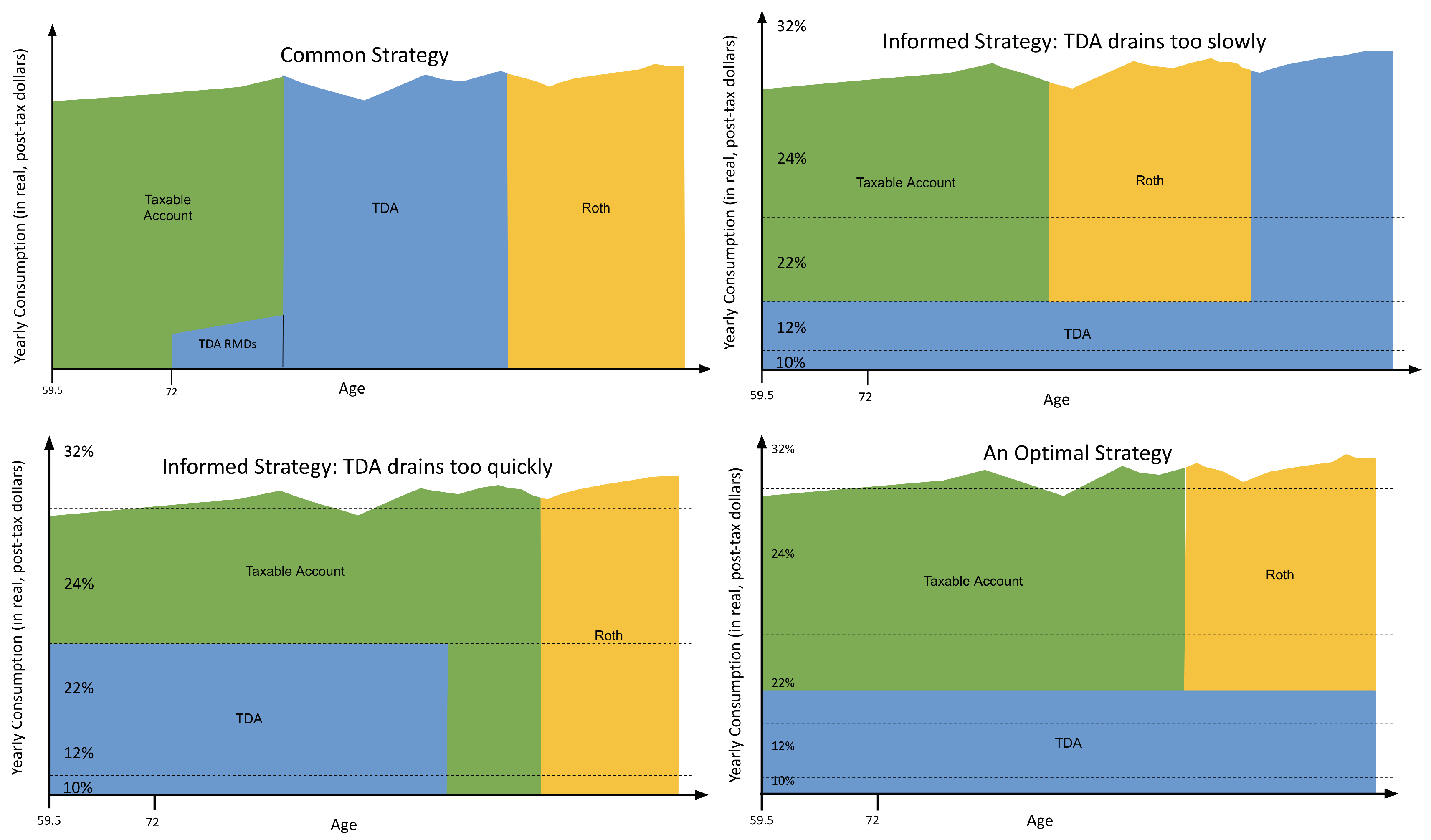
It is quite common for retirement planning books (e.g., Lange (2009), Rodgers (2009), Solin (2010), and Larimore et al. (2011)) and major investment firms (e.g., Fidelity (2015), Jaconetti and Bruno (2008), and Vanguard (2016)) to recommend a “common strategy” for withdrawal sequencing during retirement; that is, after taking out the required minimum distributions (RMDs) from the TDA account, the retiree should satisfy their remaining consumption needs by first draining their taxable account, then their TDA, and finally their Roth (see the upper left panel in Figure 1).

On occasion, a variation of the common strategy is recommended where the Roth is drained before the TDA instead of the other way around. There is a reason for the uncertainty in the sequencing of the TDA and Roth: In a constant (flat) tax rate environment for the TDA, the order in which the TDA and the Roth are removed actually makes no difference. Compelling examples of this were shown in Horan (2006a) and Spitzer and Singh (2006). A short, but very general proof of this fact is given in DiLellio and Ostrov (2018). This means that for TDA and Roth decumulation, the optimal strategy for investors is solely to reduce the tax rate for their TDA distributions, meaning they should take advantage of the lowest income tax brackets as much as possible.

Given this, Horan, in Horan (2006a) and Horan (2006b), proposed an “informed strategy” for TDA and Roth decumulation. In the informed strategy, distributions are taken from the TDA up to the top of a specific tax bracket and the Roth account is used for any additional consumption that needs to be satisfied. Should the Roth or TDA become exhausted, the other account must be used to cover all consumption needs in future years. This was expanded in Sumutka et al. (2012) to include taxable accounts. This expanded informed strategy is, as before, to take distributions from the TDA up to the top of a specific tax bracket, but to satisfy any additional consumption, the investor drains the taxable account first, then the Roth, then the TDA. We note that since our goal is to optimize the probability of investor solvency, draining the taxable account first is desirable because that minimizes capital gains taxes. If our goal was to optimize a bequest, we would need to consider the fact that capital gains are forgiven at death, which can make the optimal tax strategy far more complicated (e.g., see DiLellio and Ostrov (2018)).

A question that naturally arises with the informed strategy is which tax bracket to choose. If the tax bracket is too low, TDA distributions in later years will be at high tax rates (see the upper right panel in Figure 1). If the tax bracket is too high, the TDA will be exhausted early and therefore unable to take advantage of lower tax brackets in later years (see the lower left panel in Figure 1). We note that tax bracket limits are adjusted by inflation in the tax code, therefore we use real dollars in Figure 1, which means the TDA consumption is constant over time in the graph when the consumption level stays at the top of the chosen tax bracket.

The optimal strategy that we propose and use here is to move beyond the tax bracket limitations in the informed strategy and simply choose the optimal constant TDA consumption level, L, leading to the lower right panel in Figure 1. This is akin to the approach taken in DiLellio and Ostrov (2017), where L is found analytically for deterministic returns, a known time of death, and no taxable account. In this paper, we have stochastic returns, a distribution for the time of death, and a taxable account, so the optimal constant TDA level, L, must be determined numerically. Since this is just a single number, as opposed to a function over time, we can use standard optimization techniques to find the optimal value of L. Even better, the assumption of a constant L, even in our current stochastic context, is quite reasonable: Once L is optimized, we maintain results that look like the lower right panel in Figure 1 over a rather wide range of typical investor outcomes, as we will see later.

We are also able to accommodate other sources of income. Sources subject to no tax can simply be subtracted from the (post-tax) consumption needs of the investor. Sources subject to income tax can be added to the bottom of the graph in Figure 1 before the TDA is considered. One can think of these sources subject to income tax as looking like a sandy shore with the blue water of the TDA then being poured on top of the shore until the water level reaches L. We note that while we think of L as a post-tax level in the context of Figure 1, in this paper we report L in terms of its corresponding pre-tax value since we normally think about income tax brackets and sources subject to income tax in pre-tax terms.

We further tweak our withdrawal sequencing in two other ways. The first is that we always make certain that RMDs are distributed from the TDA each year, which can force the TDA distributions to rise above level L in some years. The second is that we take advantage of Roth conversions as was done in Cook et al. (2015). That is, as soon as possible, we convert all of the TDA distribution except for RMDs to the Roth account (since RMDs cannot legally be converted) and address the resulting additional consumption need this leaves by using withdrawals from the taxable account. This drains the taxable account more quickly, further reducing capital gains.

4. The Model and Assumptions

In this section, we detail our model. As discussed in Section 2, we determine the optimal investment strategy first, using dynamic programming. The details of this approach, including how to accommodate the mortality table, are contained in Appendix A. We note again that dynamic programming computes the optimal investment strategy by evolving it chronologically backwards in time. This is important because the optimal strategy depends on future choices, which only a backwards-in-time method has access to.

This is followed by determining the optimal tax strategy. Since we must consider the different taxation rules that apply to each of the three different accounts, and these can become complicated and depend on knowledge of past choices, we employ Monte Carlo methods, which evolve forwards in time so that we can account for path dependence. That is, our overall scheme for investment optimization followed by tax optimization is a “backwards-forwards” algorithm.

After the investment optimization is performed in the backwards part of the algorithm, we know the optimal investment allocation at any time t, given the post-tax worth of the overall portfolio at that time. Unfortunately, since we employ Monte Carlo methods for tax optimization, which evolve forwards in time, we can only know the pre-tax worth of the three accounts, not their post-tax worth, since the tax rates that will be applied in the future are not known in the present. Therefore, we must estimate the post-tax worth from our knowledge of the present. This estimate is accomplished in two phases.

Phase 1 of the post-tax estimate: In the first phase we determine an initial estimate for the post-tax worth of the overall portfolio by adding the pre-tax worth of each account, after removing an estimate of the taxes that will be levied on each account. Specifically, we sum: (1) The worth of the Roth, which has no taxes, (2) the worth of taxable bonds, after income taxes have been removed from any interest generated that year, (3) the worth of taxable stock, after applying a capital gains rate (usually 15%) to all capital gains currently in the taxable stock account, and (4) the worth of the TDA, after taking out taxes from the entire TDA at the overall rate calculated for that year’s TDA distribution.

Phase 2 of the post-tax estimate: Since our initial approximation for the post-tax worth of the portfolio is imperfect, we add a second phase to form our final approximation. In this second phase, we simply multiply the initial approximation generated in the first phase by a constant conversion correction factor, $\gamma$, that we will look to optimize. The product of $\gamma$ with our initial approximation forms our final approximation for the overall post-tax worth of the portfolio, which is then used to generate the optimal investment selection for the investor from our dynamic programming results.

This means we have two numbers, L and $\gamma$, to optimize. Were the initial post-tax approximation perfect, we would find that $\gamma =1$. In practice, we see optimum numbers like $\gamma =0.95$ more often.

Within our optimization algorithm for L and $\gamma$, we need a model for computing taxes. Our taxation model is an extensive mathematization of the federal tax code for computing income taxes and capital gains taxes. This includes laws for taxation on the following sources:

• Earned income, TDA withdrawal income, and interest income from the taxable bond account, all of which are taxed as regular income using federal income tax brackets and rates;
• TDA contributions, which are deducted from regular income, and annual standard deductions or projected itemized deductions;
• Income from realized capital gains from the taxable stock account, which is taxed using capital gains tax brackets and rates that are affected by the investor’s regular income;
• Net investment income tax (NIIT) for wealthier investors;
• Social Security income, which has particularly complicated taxation rules in that the amount that is subject to being taxed as regular income depends on the other sources of regular income and sources of capital gains income listed above, which then affects the overall taxation rates for these other sources of income.

As they vary, we do not include state or local taxes in this paper, although these generally can be easily accommodated for any specific locality.

We make a number of simplifying assumptions that, for most investors, involve taxation effects that are much smaller than those determined by the taxation model for income and realized capital gains above:

• We assume all capital gains are long term. We ignore capital losses. We ignore the effect of dividends;
• For simplicity, we calculate gains using the average cost basis method. Although LIFO (Last In, First Out) is more tax efficient, the difference is small (see Das et al. (2017), for example);
• We allow no withdrawals from the TDA nor Roth before age 59.5, even though withdrawals of contributions to Roth accounts can often be made without a penalty.

As stated earlier, investors can and should take advantage of these smaller features of the tax code (e.g., they should harvest capital losses, they should make withdrawals from the taxable stock account using LIFO, etc.). However, we will show that even the larger tax effects we do consider only have a second-order impact on the optimized strategy when compared to the first-order tax effects of the investment strategy. Therefore, it makes little sense to worry about the effect of these smaller aspects of the tax code, since they are third-order effects in the context of this paper.

We assume, as in Figure 1, that current tax bracket rates will continue to hold and that the bracket limits will continue to be adjusted by inflation, as current tax law requires. Of course tax bracket rates and limits may be changed by subsequent legislation, as we discuss in the conclusions section.

We consider the effect of our taxation model on 10,000 Monte Carlo trials, subject to optimized investments as they evolve chronologically forwards in time. The values of L and $\gamma$ maximizing the probability of remaining solvent for these trials are determined using the Nelder–Mead algorithm, with the constraint that $L\ge 0$. While this constraint is rarely needed, there are cases where the constraint keeps the algorithm from straying and wasting computational time.

5. Results

5.1. Available Investments

For the examples in this section, we have used daily historical returns from the 20-year period between January 1998 to December 2017 for index funds representing U.S. Bonds, International Stocks, and U.S. Stocks2 to determine the expected returns and covariance matrix for these three index funds. These are given in

Table 1. Summary statistics on returns from January 1998 to December 2017 for our three index funds.

Index Fund Category	Mean Return	Covariance Matrix of Returns
U.S. Bonds	0.0493	0.0017	$-0.0017$	$-0.0021$
International Stocks	0.0770	$-0.0017$	0.0396	0.03086
U.S. Stocks	0.0886	$-0.0021$	0.0309	0.0392

, and are then used to determine the efficient frontier for these three index funds.

The range for $\mu$ is restricted so that ${\mu }_{min}\le \mu \le {\mu }_{max}$. We have chosen ${\mu }_{min}=0.0526$ to correspond to the lowest possible portfolio standard deviation on the efficient frontier, which is $\sigma =0.0374$. We have chosen ${\mu }_{max}=0.0886$, the highest mean return of the three index funds, so as to discourage long-short portfolios. This corresponds to $\sigma =0.1954$ on the efficient frontier. These numbers are realistic, matching those in related research (see, for example, Exhibit 5 in Wang et al. (2011)).

We consider 15 portfolios on the efficient frontier whose $\mu$ values are equally spaced over the interval $[{\mu }_{min},{\mu }_{max}]$. The weights for the three index funds in each of these investment portfolios, labeled portfolio 0 to portfolio 14, are given in

Table 2. The portfolio weights in the three index funds for our 15 portfolios on the efficient frontier, from the most conservative (portfolio 0) to the most aggressive (portfolio 14). Both long-only and long-short portfolios are permissible.

	Portfolio Weights
Portfolio Number	U.S. Bonds	International Stocks	U.S. Stocks
0	0.9098	0.0225	0.0677
1	0.8500	0.0033	0.1467
2	0.7903	−0.0160	0.2257
3	0.7305	−0.0352	0.3047
4	0.6707	−0.0545	0.3837
5	0.6110	−0.0737	0.4628
6	0.5512	−0.0930	0.5418
7	0.4915	−0.1122	0.6208
8	0.4317	−0.1315	0.6998
9	0.3719	−0.1507	0.7788
10	0.3122	−0.1700	0.8578
11	0.2524	−0.1892	0.9368
12	0.1927	−0.2085	1.0158
13	0.1329	−0.2277	1.0948
14	0.0731	−0.2470	1.1738

. At each year and each value of the post-tax portfolio worth in the discrete state space, the dynamic strategy determines which of these 15 portfolios is optimal.

5.2. Three Example Investors

We consider three individual investors who have considerably different financial circumstances. Unless otherwise specified, for all three investors:

• The current age of the investor, defined as time $t=0$, corresponds to the year 2020.
• The rate of inflation is assumed to be 3% each year. Note: All monetary values throughout the remainder of this paper, unless specified as being nominal, will be expressed in $t=0$ dollars.
• We assume the investor elects to use the standard deduction for income taxes each year.
• We assume that the investor retires at age 65 and then immediately starts to collect Social Security.
• The investor’s mortality probability is determined by the 2020 IRS unisex mortality table.3
• We use a maximum age of 110. That is, we assume that the probability of surviving past 110 is sufficiently small that it can be ignored.

Specific parameter values for each of the investors are given in

Table 3. Parameter values for the three example investors. All monetary values are in $t=0$ dollars. All annual amounts adjust with inflation, which is assumed to be 3%.

Parameter	Investor #1	Investor #2	Investor #3
Current age ($t=0$)	40	55	65
Initial ($t=0$) TDA worth	$30,000	$100,000	$5,000,000
Initial Roth worth	$20,000	$50,000	$2,500,000
Initial taxable stock worth	$5000	$50,000	$1,000,000
Initial basis in taxable stock	$3000	$40,000	$200,000
Initial taxable bond worth	$5000	$30,000	$1,000,000
Annual pre-retirement (age 65) income (in pre-tax dollars)	$60,000	$100,000	N/A
Annual pre-retirement consumption (in post-tax dollars)	$50,000	$80,000	N/A
Annual pre-retirement TDA contribution	AUI4	$5000	N/A
Annual pre-retirement Roth contribution	$0	$5000	N/A
Annual post-retirement income (in pre-tax dollars)	$0	$20,000	$0
Annual post-retirement consumption (in post-tax dollars)	$40,000	$80,000	$400,000
Annual Social Security (starting at age 65)5	$18,132	$25,956	$34,284

. In the interest of simplicity, each investor uses annual quantities that are constants (in real dollars) that only change at retirement. However, our program is able to optimize for any desired functions of time in place of these.

5.3. Optimal Investment Strategy for the Three Example Investors

The optimal investment strategies determined with dynamic programming for our three example investors are shown as heat maps in Figure 2. These results show important qualitative behavior. Prior to retirement at age 65, an investor with a lot of money and time simply needs to make sure they do not lose too much of their wealth in order to stay solvent during their lifetime. Therefore, they choose conservative investments, represented by the light colors. As their wealth decreases or their time until retirement decreases, they optimally select progressively more aggressive investments. After retirement at age 65, a similar philosophy holds, except that the need to be more aggressive decreases as life expectancy decreases. This decrease is reflected by the slope of the dark region at the top of the graph becoming increasingly negative as time progresses past retirement.

The white region that starts in the lower part of each graph at age 65, the first year of retirement, corresponds to cases where the investor does not have enough money to cover that year’s consumption costs, which are taken out at the beginning of the year. Since they go bankrupt immediately, the investment portfolio choice is irrelevant, and we get random results for the optimal portfolio. Since these random results are both distracting and meaningless, they are covered in white, except for a small band just above the white region where random colors can be seen.

Just above the random band is a dark band that corresponds to being able to afford the current year’s consumption, but having so little left that an aggressive portfolio is the only hope of attaining the amount needed for next year’s consumption. The small light colored blocks from ages 60 to 64 correspond to the investor needing to stay in conservative portfolios so as to ensure they will have enough money to be able to afford a single year of consumption at age 65 and not end up below the dark band. The light band just above the dark band that starts at age 65 corresponds to the need for a conservative portfolio to ensure maintaining enough funds for both the current year and the next year. With a little more money, the investor is likely to be able to maintain enough money for both years’ consumption needs, and possibly attain a third year of consumption, with an aggressive portfolio, so we see another dark band. This pattern continues for yet another year of meeting consumption needs as we get to higher wealth values. We note that the positive slope of these bands corresponds to the fact that consumption needs increase by the rate of inflation and the graph is in nominal dollars. We also note that all of these light colored lines and blocks result from the fact that our model removes consumption needs all at once at the beginning of each year. In a more realistic scenario, money would be continuously withdrawn, in which case these light colored lines and blocks would disappear from Figure 2.

5.4. Optimal Tax Strategy for the Three Example Investors

The optimal tax strategies for the three example investors are given in

Table 4. Optimal tax strategies for the three example investors, along with the optimal probability of solvency found using both the optimal investment strategy given in Figure 2 and the optimal tax strategy given here. L is the desired amount of consumption (in pre-tax, $t=0$ dollars) from sources subject to income tax, such as the TDA, earned income, Social Security, and taxable bond interest. $\gamma$ is a pre-tax to post-tax conversion correction factor.

Parameter	Investor #1	Investor #2	Investor #3
Optimal L value (in pre-tax dollars)	$11,900	$21,400	$220,000
Optimal $\gamma$ value	0.935	0.971	0.949
Optimal Probability of Solvency	68.3%	40.5%	90.6%

, along with the optimal probability of solvency that is determined from combining the optimal investment strategy in Figure 2 with the optimal tax strategy. The results in Table 4 reflect expected qualitative behavior.

Table 5. 2020 tax brackets for a single investor. The income range for these brackets is adjusted by our inflation rate of 3% in later years, reflecting current tax law.

Tax Bracket	Income Range (in Pre-Tax Dollars)
10%	$0–$9875
12%	$9875–$40,125
22%	$40,125–$85,525
24%	$85,525–$163,300
32%	$163,300–$207,350
35%	$207,350–$518,400
37%	>$518,400

gives the tax brackets used by the model at $t=0$, which corresponds to the year 2020. For Investor #1, the optimal L value, $11,912, is just above the 10% tax bracket. This corresponds to the fact that after the standard deduction of $12,400 (in $t=0$ dollars) is taken into account, the investor’s consumption will never push the investor past the 12% tax bracket. That is, the 10% bracket is taken full advantage of here, knowing that the maximum tax rate will be 12%. For Investor #2, the optimal L is near the middle of the 12% tax bracket, which means rarely entering the 22% bracket later while maintaining a continued ability to take advantage of the 10% bracket. For Investor #3, the optimal L is just above the 32% bracket, which minimizes the effect of the 35% and 37% brackets. As stated earlier, the optimal values of $\gamma$, our pre-tax to post-tax conversion correction factor, typically range between 0.90 and 1.00, as we see with all three investors here.

5.5. Two Example Paths Demonstrating the Properties of the Optimal Investment and Optimal Tax Strategies

A Monte Carlo path that remains solvent. In Figure 3 we analyze one of the 10,000 Monte Carlo trials for Investor #1 under the optimal strategy to better understand the optimal strategy’s features. The top panel in Figure 3 shows the worth of each of the three accounts over time. The middle panel shows the annual consumption from the three accounts. The bottom panel shows how the optimal investment portfolio used for all three accounts evolves over time. The middle panel exhibits “negative TDA consumption” values prior to age 65, which are actually the TDA contributions that are made from any unconsumed income during these years. From age 65 to age 67, the TDA withdrawals needed to attain the optimal level $L=$ $11,912 (in $t=0$ dollars) are converted to the Roth account, which creates “negative Roth consumption” in these years, while the investor’s consumption needs are addressed using the taxable account. After age 67 this is no longer possible since the taxable account is drained. From age 68 to age 71, we consume from the TDA to attain level L, with the remainder of the consumption coming from the Roth. Note the straight line segments during this period in the middle panel, where the slight positive slopes are due to inflation. From age 72 on, TDA consumption is driven by the RMDs, since RMD consumption is higher than level L. Again, the remaining consumption needs are addressed with the Roth. Due to generally good stock returns in this case, the investor has plenty of money to remain solvent, even though they live to age 98. This is reflected in the bottom panel by the optimal investment strategy being highly aggressive at first and then becoming very conservative by the time the investor reaches their late 40s.

A Monte Carlo path that ends in bankruptcy. We next consider how our optimal tax strategy fits with the desired lower right panel of Figure 1, in which we have a horizontal line over time that corresponds to a constant taxable withdrawal level in real dollars, and, should the investor become bankrupt, money in the TDA and the Roth account runs out at the same time. With our optimal tax strategy, this generally holds in the years when bankruptcy is most likely. To see this we consider Investor #3, but with a single projected time of death at age 90 in the place of our mortality distribution, so bankruptcy, when it happens, is most likely just before age 90, since the investor normally remains solvent. By changing to this projected death at age 90, the optimal L becomes $262,000 and the optimal $\gamma$ becomes 0.977. We show the optimal results for one of our 10,000 Monte Carlo trials in Figure 4.

The behavior in Figure 4 has qualitative similarities to Figure 3 in its initial years. We see a conversion from the TDA to the Roth from age 65 until age 69, when the taxable stock needed to cover the investor’s consumption needs runs out. Again, this conversion helps drain the taxable account early, minimizing capital gains taxes. From age 70 onwards, the investor consumes TDA so as to attain $L=$ $262,000, with the remainder of the investor’s consumption needs addressed by the Roth. This corresponds to the smooth curves in the consumption graph from age 70 to age 84, reflecting the desired constant taxable withdrawal level in real dollars. During this period, we see the investor’s TDA worth going down, not up as in Figure 3, reflecting poorer returns in this case. This means smaller RMDs, so that L, as opposed to the RMDs, is driving TDA consumption during these years, unlike in Figure 3. The diminishing overall wealth of the investor leads, as it should, to more aggressive investments to maintain solvency, as shown in the bottom panel of Figure 4. As desired, we note that we essentially run out of the TDA and Roth at the same time. Only in the year before bankruptcy at age 86 do we have TDA funds, but no Roth money. In general, we find that that these two accounts generally become depleted within a year or two of each other over a rather wide range of bankruptcy times, conforming well to the desired behavior shown in the lower right panel of Figure 1.

5.6. Comparing Our Optimal Investment Strategy to a Target Date Fund and a Static Portfolio

To judge the effect of our optimized investment strategy on the probability solvency, we compare it (1) to a standard target date fund strategy shown in

Table 6. The standard glide path strategy used for the target date fund in this section.

Age Range	40–44	45–49	50–54	55–59	60–64	65–69	70–74	≥75
U.S. Bonds	9%	17%	27%	34%	42%	53%	67%	70%
International Stocks	36%	33%	29%	26%	23%	19%	13%	12%
U.S. Stocks	55%	50%	44%	40%	35%	28%	20%	18%

, which uses the same three index funds that were available to our optimized investment strategy and (2) to a static portfolio strategy that annually rebalances the three index funds so as to maintain 60% U.S. Bonds, 10% International Stocks, and 30% U.S. Stocks.

For each of these three investment strategies, with each of our three example investors, we can determine and apply the optimal tax strategy, which allows us to compare the effect of the investment strategies on the probability of solvency. The results of this comparison are given in

Table 7. The effect of the investment strategy on the optimal probability of solvency. In each of the nine cases shown here, we present the optimal solvency probability after determining and applying the optimal tax strategy. The values of L and $\gamma$ in the optimal tax strategy are not strongly affected by which investment strategy is selected. Parameter values for Investors #1, #2, and #3 are given in Table 3.

Investment Strategy	Investor #1	Investor #2	Investor #3
Our optimal dynamic programming investment strategy	68.3%	40.5%	90.6%
Target date fund investment strategy from Table 6	51.8%	23.9%	85.9%
Static portfolio strategy (60% U.S. Bonds,
10% Intl. Stock, 30% U.S. Stock)	43.2%	19.8%	87.2%

. We see from this table that our approach significantly outperforms both the target date fund and static portfolio strategies, leading to noticeably higher likelihoods that the investor remains solvent throughout their lifetime.

If we again replace our mortality distribution table with a projected time of death at age 90, the outperformance of our optimal investment strategy becomes even more striking, as we see in

Table 8. The effect of the investment strategy on the optimal probability of solvency when the investor is projected to die at age 90. As before, in all cases we determine and apply the optimal tax strategy.

Investment Strategy	Investor #1	Investor #2	Investor #3
Our optimal dynamic programming investment strategy	63.9%	32.2%	96.6%
Target date fund investment strategy from Table 6	33.9%	4.0%	84.6%
Static portfolio strategy (60% U.S. Bonds,
10% Intl. Stock, 30% U.S. Stock)	18.3%	0.9%	85.8%

. The dynamic programming approach is able to take advantage of the certainty of the portfolio horizon here, in contrast to the uncertainty inherent in the mortality distribution, which means more information for dynamic programming to exploit. The target date fund and the static portfolio strategies, on the other hand, are not altered by changing from a mortality distribution to a specific date, so it is unsurprising that we see more outperformance when applying our method to this case.

5.7. The Robustness of Our Optimal Tax Strategy to Changes in L and $\gamma$

In

Table 9. The effect of varying the values of L and $\gamma$ from their optimal (in bold) values on the solvency probability for each of our three example investors.

Investor #1	Value of $\gamma$
Value of L	0.88	0.90	0.92	0.935	0.94	0.97	1.00
$0	67.4%	67.4%	67.3%	67.3%	67.2%	66.9%	66.6%
$5000	67.6%	67.7%	67.7%	67.6%	67.5%	67.3%	66.9%
$10,000	67.9%	68.1%	68.2%	68.2%	68.1%	67.9%	67.6%
$11,900	67.9%	68.0%	68.2%	68.3%	68.0%	67.8%	66.9%
$20,000	66.9%	67.1%	67.2%	67.4%	67.4%	67.4%	67.2%
$30,000	67.0%	67.3%	67.4%	67.6%	67.7%	67.5%	67.4%
$50,000	66.8%	66.9%	67.1%	67.2%	67.2%	67.1%	67.0%
Investor #2	Value of $\gamma$
Value of L	0.90	0.93	0.96	0.971	0.98	0.99	1.00
$0	40.3%	40.2%	40.2%	40.2%	40.2%	40.1%	40.1%
$10,000	40.3%	40.2%	40.2%	40.2%	40.2%	40.1%	40.1%
$20,000	40.3%	40.2%	40.2%	40.2%	40.2%	40.1%	40.1%
$21,400	40.3%	40.4%	40.4%	40.5%	40.4%	40.3%	40.2%
$25,000	40.1%	40.1%	40.3%	40.4%	404.%	40.3%	40.2%
$50,000	40.0%	40.1%	40.3%	40.4%	40.4%	40.3%	40.2%
$100,000	39.3%	39.4%	39.6%	39.6%	39.6%	39.6%	39.4%
Investor #3	Value of $\gamma$
Value of L	0.90	0.92	0.94	0.949	0.96	0.98	1.00
$0	89.2%	89.1%	89.0%	89.0%	88.8%	88.7%	88.7%
$100,000	89.9%	90.0%	90.0%	89.9%	89.8%	89.8%	89.7%
$200,000	90.1%	90.4%	90.4%	90.4%	90.4%	90.2%	90.1%
$220,000	90.1%	90.5%	90.5%	90.6%	90.4%	90.4%	90.2%
$250,000	89.9%	90.1%	90.4%	90.5%	90.5%	90.3%	90.3%
$350,000	88.7%	89.0%	89.4%	89.4%	89.5%	89.5%	89.6%
$500,000	87.8%	88.1%	88.3%	88.4%	88.5%	88.5%	88.6%

, we see the effect on the three example investors of altering L and $\gamma$ away from their optimal values, which are in bold. The range of $\gamma$ goes from 0.88 to 1.00 for Investor #1 and from 0.90 to 1.00 for Investor #2 and Investor #3. The range of L goes from 0 to full consumption for Investor #1 and Investor #2 and from 0 to near full consumption for Investor #3. The key observation is how small the solvency probability variation is in each case. The solvency probabilities for Investor #1 stay within a 1.7 percentage point range, for Investor #2, it is a 1.2 percentage point range, and for Investor #3, it is a 2.8 percentage point range.

Some of the lack of variation in Table 9 is due to RMDs supplanting the relevance of the L value after age 72 in many cases. However, even for Investor #3 with a projected death at age 90, which governs the path exhibited in Figure 4 where RMDs never supplant the L value, we still only have a 4.6 percentage point range, as shown in

Table 10. The effect of varying the values of L and $\gamma$ from their optimal (in bold) values on the solvency probability for Investor #3 if the investor’s date of death is projected to be at age 90.

Investor #3,
Age 90 Death	Value of $\gamma$
Value of L	0.90	0.93	0.96	0.977	0.98	0.99	1.00
$0	95.2%	95.1%	94.3%	93.5%	93.3%	92.7%	92.0%
$100,000	95.5%	95.7%	95.1%	94.5%	94.3%	93.8%	93.3%
$200,000	95.8%	96.2%	95.9%	95.3%	95.2%	94.8%	94.2%
$262,000	94.5%	95.7%	96.2%	96.6%	96.6%	96.5%	96.5%
$300,000	93.9%	95.2%	95.9%	96.0%	96.1%	96.2%	96.2%
$400,000	92.9%	94.0%	95.0%	95.2%	95.2%	95.3%	95.3%
$500,000	92.1%	93.3%	94.5%	94.6%	94.7%	94.7%	94.8%

. For Investor #1 and Investor #2 with projected deaths at age 90, the percentage point range also increases to 7.0 and 2.0 percentage points respectively. Therefore, the tax optimization strategy is quite robust to changes in L and $\gamma$.

Comparing this exhibited range for varying the tax strategy, which is, at most, 7.0 percentage points, with Table 7 and Table 8, where the exhibited range for varying the investment strategy is as high as 45.6 percentage points, clearly establishes our key finding that optimizing the investment strategy is far more important to maximizing an investor’s solvency probability than optimizing their tax strategy. Again, this should not be interpreted to mean that tax strategy optimization is unimportant. Investment strategy optimization increases the probability of a better outcome, whereas the better outcomes generated by tax strategy optimization are generally far more stable, directly creating additional money for an investor. While the amount of this additional money is generally not large enough to provide the investor with the additional resources needed to avoid a bankruptcy that would otherwise occur during the investor’s lifetime, there is no reason to ignore the arbitrage-like possibilities that improved tax strategies can provide investors.

That being said, our analysis makes it clear why it is important to first worry about determining the optimal investment strategy, since it has such a big effect, and then worry about finding the optimal tax strategy that conforms to this optimal investment strategy. This further justifies our algorithm’s approach, since we first use dynamic programming to determine the optimal investment strategy and, only after that, do we move on to using Monte Carlo simulation and numerical optimization to determine the optimal tax strategy.

5.8. Comparative Statics with the Three Example Investors

In this subsection we consider the effect on the optimal probability of solvency when we alter some of the example investors’ parameters, one at a time.

Effect of varying the initial worth of the TDA: In

Table 11. The effect on Investor #1 of varying the initial worth of the TDA from its normal value (in bold).

Initial	Optimal Probability of Solvency	Optimal Probability of Solvency
TDA Worth	(Mortality Table)	(Projected Death at Age 90)
$0	57.3%	50.5%
$15,000	63.3%	58.0%
$30,000	68.3%	63.9%
$50,000	73.6%	71.2%
$75,000	79.3%	78.0%
$100,000	84.1%	84.0%
$200,000	95.3%	96.8%
$300,000	99.3%	99.5%
$500,000	100.0%	100.0%

we look at how Investor #1’s optimal probability of solvency changes if they saved different amounts of TDA money prior to $t=0$. This is tabulated both for the normal mortality table and when the investor is projected to die at age 90. We note that changes in TDA savings as small as $30,000–$40,000 can change the optimal probability of solvency by more than 10 percentage points. By comparison, recall that our tax optimization generates, at most, 7.0 additional percentage points for the optimal solvency probability. From Table 11 we can see that this corresponds to about $15,000–$20,000 additional initial TDA dollars. That is, for Investor #1, tax optimization generates a certainty equivalent in the range of $15,000–$20,000 pre-tax dollars at $t=0$.

Effect of varying income: We look at the effect on Investor #2 of having their pre-retirement income vary in

Table 12. The effect on Investor #2 of varying the pre-retirement income, in $t=0$ pre-tax dollars, from its normal value (in bold).

Annual Pre-Retirement Income	Optimal Probability of Solvency
$80,000	8.1%
$90,000	27.8%
$100,000	40.5%
$110,000	52.6%
$125,000	67.8%
$150,000	85.2%

and their post-retirement income vary in

Table 13. The effect on Investor #2 of varying the post-retirement income, in $t=0$ pre-tax dollars, from its normal value (in bold).

Annual Post-Retirement Income	Optimal Probability of Solvency
$0	25.3%
$10,000	31.6%
$20,000	40.5%
$30,000	52.8%
$40,000	71.1%
$50,000	94.3%

. Since these are annual amounts—over 10 years in the case of pre-retirement income, and generally more than that for post-retirement income—they have a significant effect on the optimal solvency probability. In the pre-retirement income case in Table 12, the optimal value of L decreases from $47,300 when the pre-retirement income is $80,000 to L = $14,100 as the pre-retirement income increases to $150,000. This follows from the drastic change in the optimal solvency probability. When this probability is small (e.g., 8.1%), the early bankruptcies mean the age intervals shown on the horizontal axes in Figure 1 are small. To maintain the desired constant withdrawal level corresponding to L in the lower right panel of Figure 1, we require L to be high. On the other hand, when the solvency probability is large, the age intervals become longer, so L needs to decrease to maintain a constant withdrawal level over the investor’s lifetime.

Effect of varying consumption: The flip side of varying income is to alter consumption. The effect on Investor #2 of changing their pre-retirement consumption is shown in

Table 14. The effect on Investor #2 of varying the pre-retirement consumption, in $t=0$ post-tax dollars, from its normal value (in bold).

Annual Pre-Retirement Consumption	Optimal Probability of Solvency
$60,000	69.0%
$70,000	55.9%
$75,000	48.8%
$80,000	40.5%
$90,000	23.9%
$100,000	4.8%

, and the effect of changing their post-retirement consumption is shown in

Table 15. The effect on Investor #2 of varying the post-retirement consumption, in $t=0$ post-tax dollars, from its normal value (in bold).

Annual Post-retirement Consumption	Optimal Probability of Solvency
$60,000	84.1%
$70,000	57.5%
$75,000	48.3%
$80,000	40.5%
$90,000	29.2%
$100,000	22.7%

. We note that dollar changes in the consumption have a stronger effect than equivalent dollar changes to income. This is because consumption dollars are post-tax while income dollars are pre-tax, and therefore worth less after taxes are subtracted.

Effect of varying the starting date for collecting Social Security: When is it optimal to start collecting Social Security? The general wisdom is that an unmarried investor should wait as long as possible, even though fewer than 5% of retirees actually do wait until the maximum age of 70.6 However given that our algorithm optimally invests money, perhaps it is better to take money out from Social Security earlier, because that allows the money to be optimally invested earlier. In

Table 16. The effect on Investor #1 of varying the start of collecting Social Security from its normal age (in bold).

Social Security	Annual Social Security	Optimal Probability
Starting Age	(t = 0 dollars)	of Solvency
62	$14,088	66.2%
63	$15,204	66.7%
64	$16,536	67.2%
65	$18,132	68.3%
66	$19,752	68.6%
67	$21,504	68.7%
68	$23,472	69.3%
69	$25,476	69.9%
70	$27,516	70.5%

, we have used Social Security’s website (https://www.ssa.gov, accessed on 17 August 2020) to generate the optimal probability of solvency for Investor #1 should they decide to begin collecting Social Security at any year between the minimum age, 62, and the maximum age, 70. We see from this table that the general wisdom still holds for Investor #1. That is, the optimal Social Security strategy is still to wait as long as possible, even when exploiting the optimal investment strategy and the optimal tax strategy. Of course, this assumes our current, standard mortality table. Should an investor have health issues that correspond to a mortality table where an earlier death is more likely, our algorithm may indicate that the optimal Social Security starting age is earlier.

5.9. Pricing Annuities

How much, at most, should Investor #3 pay in post-tax dollars at age 65, which is $t=0$, for an annuity that, starting at age 80, pays out $100,000 post-tax $t=0$ dollars every year they remain alive? Since the purpose of an annuity is to increase the probability that the investor will remain solvent, we look to find what amount of money spent at $t=0$ for this annuity will lead to the same 90.6% optimal solvency probability that we have without the annuity. We find that if we lower the consumption from $400,000 to $300,000 starting at age 80 to reflect the $100,000 annual payout, we must reduce the initial Roth worth from $2,500,000 to $1,660,000 to maintain the 90.6% probability of solvency we had before. Therefore, the investor should pay no more than $2,500,000 − $1,660,000 = $840,000 for this annuity.

Qualified Longevity Annuity Contracts (QLACs) can be purchased from within a TDA without an immediate tax consequence, although the payouts are then taxed as income. We can therefore pose a similar question in this context. How much, at most, should Investor #3 pay in pre-tax TDA dollars at $t=0$ for an annuity that, starting at age 80, provides $100,000 of taxable income in $t=0$ dollars every year they remain alive? In this case we give the investor an income of $100,000 (in $t=0$ dollars) starting at age 80 and find that we must reduce their initial TDA worth from $5,000,000 to $4,160,000 to maintain the desired 90.6% probability of solvency. Therefore, the investor should pay no more than $5,000,000 − $4,160,000 = $840,000 for this annuity, the same value we found in the post-tax case above. In other words, at least for the case presented here, the taxation structure for the pre-tax TDA used to purchase the QLAC and the taxation structure for the income provided by the annuity are nearly identical, so the cost in pre-tax dollars of the QLAC is identical to the post-tax cost of the annuity, where the tax structure of the payment and the payouts have to be identical since neither is subject to tax.7

6. Conclusions

Both investment optimization and tax optimization are important for retirees, but they have very different mechanisms and implications. Investment optimization is probabilistic in nature, balancing risk and return. Tax optimization is path-dependent and far more deterministic, making choices that have known tax consequences. Investment optimization and tax optimization have generally been performed independently of each other, despite the fact that they affect each other. In this paper we have shown that the effect of investment optimization on the probability that an investor will remain solvent throughout their lifetime is significantly higher than the effect of tax optimization. This means that investment optimization can reasonably be done with little or even no thought to tax optimization, but tax optimization should then be done in the context of this optimized investment strategy. Tax optimization is still important, because the money generated by tax optimization is generally stable and would be foolish to ignore.

This paper presents an investment and tax optimization scheme based on this premise. In the first stage, the algorithm optimizes the investment strategy using dynamic programming in post-tax dollars, which is computed backwards in time. This optimal investment strategy is then incorporated into a second stage that optimizes the tax strategy using Monte Carlo simulation, which evolves forwards in time. The model carefully computes taxes from all typically significant sources of income and capital gains for American investors. It accommodates infusions into TDAs, Roth accounts, and taxable stock and bond accounts, and then it optimizes withdrawal allocations from these accounts to meet consumption needs. The model incorporates Social Security, standard or itemized deductions, and required minimum distributions (RMDs) from the TDA. It also minimizes capital gains taxes by using early non-RMD TDA money for Roth conversions instead of for consumption, so the taxable stock account must be drained earlier to address the investor’s consumption needs.

The sensitivity of the investor’s optimal solvency to variations in a number of parameters is explored, including pre- and post-retirement income, pre- and post-retirement consumption needs, and the initial worth of the TDA. The model may be used to compute the appropriate price for purchasing annuities using either pre-tax or post-tax money. It shows that even under the optimized investment and tax strategy, it is still generally best for unmarried investors to put off collecting Social Security as long as possible.

Of course, this assumes that Social Security payout rules are not changed by legislation in the future, and it assumes that the Social Security Trust Funds do not become depleted, resulting in lowered payouts. As stated in the introduction, for the sake of simplicity we have assumed that the tax structure does not change over time. Of course, the tax structure can and often does change over time. For example, Croce et al. (2012) and Pastor and Veronesi (2012) studied how tax changes can be triggered by changes to macroeconomic factors. It is difficult to use dynamic programming to study how to optimally invest with potential tax structure changes. This is due to the need both for an accurate stochastic model for how tax parameters, such as tax bracket limits and rates, change in the future and for the additional state space variables needed to accommodate these parameters, which quickly slows the dynamic programming calculation via the so-called “curse of dimensionality” (see Brown et al. (2017), however, for a dynamic programming approach over two periods that explores how to best allocate funds between a TDA and a Roth account). Fortunately, our method only uses dynamic programming on a post-tax basis, so it is not subject to these computational problems. Indeed, the Monte Carlo nature of our forwards-in-time tax calculations can easily be extended to accommodate just about any stochastic model for changing tax parameters over time without a change in computational speed. Furthermore, our model is particularly well suited to accommodating models such as Hassett and Metcalf (1999), where the distribution for tax parameter changes is correlated to stock returns.

This paper’s model can also be extended in a variety of other different directions. For example, the investor’s consumption needs can be made to depend on both the investor’s wealth and age, instead of just the age as we have in this paper. The dependence on wealth makes intuitive sense since an investor will generally reduce their consumption as their wealth decreases. As another example, the investor’s consumption needs can be made to be stochastic instead of deterministic to reflect any uncertainty that investors have about their future consumption needs. Another optional extension is to consider different investment portfolios in each of the investor’s three accounts to allow further tax optimization. We can also consider how to optimize the probability of being able to make a desired bequest, taking advantage of the fact that capital gains are forgiven at death. As a final example, it is possible to expand the model to married couples in addition to single investors. This requires considering the mortality distribution for the death of either spouse at first, and then the mortality distribution for the surviving spouse, as well as switching from the tax brackets for married couples to those for single individuals after the first spouse dies.

References

1. Browne, Sid. 1995. Optimal investment policies for a firm with a random risk process: Exponential utility and minimizing the probability of ruin. Mathematics of Operations Research 20: 937–58. [Google Scholar] [CrossRef] [Green Version]
2. Browne, Sid. 1997. Survival and growth with a liability: Optimal portfolio strategies in continuous time. Mathematics of Operations Research 22: 468–93. [Google Scholar] [CrossRef] [Green Version]
3. Browne, Sid. 1999. Reaching goals by a deadline: Digital options and continuous-time active portfolio management. Advances in Applied Probability 31: 551–77. [Google Scholar] [CrossRef]
4. Brown, David C., Scott Cederburg, and Michael S. O’Doherty. 2017. Tax Uncertainty and Retirement Savings Diversification. Journal of Financial Economics 126: 689–712. [Google Scholar] [CrossRef]
5. Cook, Kristen A., William Meyer, and William Reichenstein. 2015. Tax-Efficient Withdrawal Strategies. Financial Analysts Journal 71: 16–29. [Google Scholar] [CrossRef] [Green Version]
6. Croce, Mariano M., Howard Kung, Thien T. Nguyen, and Lukas Schmid. 2012. Fiscal Policies and Asset Prices. The Review of Financial Studies 25: 2635–72. [Google Scholar] [CrossRef]
7. Dammon, Robert M., Chester S. Spatt, and Harold H. Zhang. 2004. Optimal Asset Location and Allocation with Taxable and Tax-Deferred Investing. The Journal of Finance 59: 999–1037. [Google Scholar] [CrossRef]
8. Das, Sanjiv R., Daniel Ostrov, Anand Radhakrishnan, and Deep Srivastav. 2019. Dynamic Portfolio Allocation in Goals-Based Wealth Management. Computational Management Science, 1–28. [Google Scholar] [CrossRef]
9. Das, Sanjiv R., Dennis Yi Ding, Vincent Newell, and Daniel N. Ostrov. 2017. Efficient Trading in Taxable Portfolios. Journal of Investment Strategies 7: 1–40. [Google Scholar] [CrossRef]
10. DiLellio, James A., and Daniel N. Ostrov. 2017. Optimal Strategies for Traditional versus Roth IRA/401(k) Consumption during Retirement. Decision Sciences 48: 356–84. [Google Scholar] [CrossRef]
11. DiLellio, James A., and Daniel N. Ostrov. 2018. Constructing Tax Efficient Withdrawal Strategies for Retirees with Traditional 401(k)/IRAs, Roth 401(k)/IRAs, and Taxable Accounts. In Proceedings of the Academy of Finanial Services 2018 Annual Conference, Chicago, IL, USA, October 2–3; Available online: https://academyfinancial.org/resources/Documents/Proceedings/2018/F2%20DiLellio%20and%20Ostrov.pdf (accessed on 13 July 2020).
12. Employee Benefits Security Administration, and United States Department of Labor. 2019. “Private Pension Plan Bulletin Historical Tables and Graphs 1975-2017”, Contract DOLOPS14D0017. Washington, DC: EBSA. [Google Scholar]
13. Fidelity. 2015. Detailed Methodology, Retirement Income Planner. Available online: http://personal.fidelity.com/planning/retirement/pdf/rip_methodology.pdf (accessed on 18 July 2020).
14. Hassett, Kevin A., and Gilbert E. Metcalf. 1999. Investment with Uncertain Tax Policy: Does Random Tax Policy Discourage Investment? The Economic Journal 109: 372–93. [Google Scholar] [CrossRef]
15. Horan, Stephen M. 2006a. Optimal Withdrawal Strategies for Retirees with Multiple Savings Accounts. Journal of Financial Planning 19: 62–75. [Google Scholar]
16. Horan, Stephen M. 2006b. Withdrawal Location with Progressive Tax Rates. Financial Analysts Journal 62: 77–87. [Google Scholar] [CrossRef] [Green Version]
17. Jaconetti, Colleen M., and Maria A. Bruno. 2008. Spending from a Portfolio: Implications of Withdrawal Order for Taxable Investors. Vanguard Research, 1–15. Available online: https://www.ceworkshops.com/assets/images/4%20Spending%20from%20Portolio%20in%20Retirement%20-%20Vanguard%20Article%20(1).pdf (accessed on 25 November 2020).
18. Lange, James. 2009. Retire Secure! Hoboken: Wiley, ISBN 0470405317. [Google Scholar]
19. Larimore, Taylor, Mel Lindauer, Richard A. Ferri, and Laura F. Dogu. 2011. The Bogleheads’ Guide to Retirement Planning. Hoboken: Wiley, ISBN 0470919019. [Google Scholar]
20. Merton, Robert C. 1969. Lifetime Portfolio Selection under Uncertainty: The Continuous-Time Case. The Review of Economics and Statistics 51: 247–57. [Google Scholar] [CrossRef] [Green Version]
21. Merton, Robert C. 1971. Optimum consumption and portfolio rules in a continuous-time model. Journal of Economic Theory 3: 373–413. [Google Scholar] [CrossRef] [Green Version]
22. Pastor, Lubos, and Pietro Veronesi. 2012. Uncertainty about Government Policy and Stock Prices. The Journal of Finance 67: 1219–64. [Google Scholar] [CrossRef]
23. Rodgers, Rick. 2009. The New Three-Legged Stool. Hoboken: Wiley, ISBN 1592803636. [Google Scholar]
24. Solin, Daniel R. 2010. The Smartest Retirement Book You’ll Ever Read. New York: Perigee Trade, ISBN 0399536345. [Google Scholar]
25. Spitzer, John J., and Sandeep Singh. 2006. Extending Retirement Payouts by Optimizing the Sequence of Withdrawals. Journal of Financial Planning 19: 52–61. [Google Scholar]
26. Sumutka, Alan R., Andrew M. Sumutka, and Lewis W. Coopersmith. 2012. Tax-Efficient Retirement Withdrawal Planning Using a Comprehensive Tax Model. Journal of Financial Planning 25: 41–52. [Google Scholar]
27. Vanguard. 2016. How to Turn Retirement Savings into Retirement Income. Available online: https://retirementplans.vanguard.com/web/enc/pdfs/RILongBroc.pdf (accessed on 28 October 2020).
28. Wang, Hungjen, Anil Suri, David Laster, and Himanshu Almadi. 2011. Portfolio Selection in Goals-Based Wealth Management. Journal of Wealth Management 14: 55–65. [Google Scholar] [CrossRef]
Short Biography of Authors
Jrfm 14 00285 i001Sanjiv R. Das is a William and Janice Terry Professor of Finance and Data Science at the Leavey School of Business at Santa Clara University.
Jrfm 14 00285 i002Dan Ostrov is a Professor of Mathematics and Computer Science at Santa Clara University.
Jrfm 14 00285 i003Aviva Casanova is a Manager within the Client Analytics group at Franklin Templeton.
Jrfm 14 00285 i004Anand Radhakrishnan is a Vice President/Head of Digital Products within the FT Investment Solutions group at Franklin Templeton.
Jrfm 14 00285 i005Deep Srivastav is a Senior Vice President/Head of Digital Solutions within the FT Investment Solutions group at Franklin Templeton.
Figure 1. Four tax strategies. All consumption amounts are in real, post-tax dollars. Upper left panel: The common strategy, withdrawing from the taxable account (plus TDA RMDs), then the TDA, then the Roth account. Upper right panel: The informed strategy for withdrawing TDA money through the 12% bracket. Lower left panel: The informed strategy for withdrawing TDA money through the 22% bracket. Lower right panel: Our strategy for optimizing the TDA withdrawal rate. The height of the blue TDA rectangle corresponds to the value of L.
Jrfm 14 00285 g001
Figure 2. Optimal investment strategies. Top panel: The optimal investment strategy for Investor #1 as a function of the investor’s age on the horizontal axis and wealth, in nominal post-tax dollars, on the logarithmic scaled vertical axis. The potential investment portfolios on the efficient frontier are numbered 0 to 14, in order of increasing aggressiveness. The darker the color in the figure, the higher the number of the optimal portfolio investment. Note that a white region starting at age 65 has been inserted to cover low wealth values where bankruptcy is guaranteed at the beginning of the year, making the investment choice during the year irrelevant. Lower left panel: The optimal investment strategy for Investor #2. Lower right panel: The optimal investment strategy for Investor #3 with small wealth values that correspond to the white region removed. Note that all three panels show similar patterns of behavior.
Jrfm 14 00285 g002
Figure 3. An example path for Investor #1 under the optimal strategy. Age is on the horizontal axis. For this example path, the investor was solvent when they died at age 98. In the top two panels, the dollar values on the vertical axes are in nominal, pre-tax dollars. Top panel: The wealth in the TDA, Roth, and taxable accounts over time. Middle panel: The annual consumption in the three accounts, where negative consumption corresponds to a contribution. Bottom panel: The optimal investment strategy over time, where portfolio 0 is the most conservative investment portfolio, portfolio 14 is the most aggressive investment portfolio, and “portfolio -1” is used to indicate the investor has passed away.
Jrfm 14 00285 g003
Figure 4. An example path for Investor #3 under the optimal strategy. In this case, instead of using mortality tables, it has been assumed that the investor’s date of death is projected to be at age 90. For this example path, the investor becomes bankrupt at age 86. As in Figure 3, age is on the horizontal axis, and in the top two panels, the dollar values on the vertical axes are in nominal, pre-tax dollars.
Jrfm 14 00285 g004