1. Introduction
The increasing financial interdependence, particularly during the current era of global economic events and financial turbulence has prompted considerable interest from market participants and academic research. While much attention has been paid to the magnitude of return and volatility spillovers across global stock markets, little is known about the foreign exchange channels, in particular, the foreign exchange markets’ channels between developed and developing countries. Some studies of this kind have investigated the return co-movements and volatility spillovers, primarily across the developed countries
Anderson et al. (
2001),
Pérez-Rodrìguez (
2006),
Boero et al. (
2011), and
Rajhans and Jain (
2015). Others have considered the regional spillover transmission and produced insignificant results.
However, given the trillions of dollars of exchange rate trading in international financial markets, it is important to fully understand and investigate in greater depth the potential spillovers of international currencies. This is an important aspect that investors must account for during the formation of their position and portfolios. Before the recent financial turmoil, the contribution of the channels of foreign exchange markets’ spillovers to the global financial instability, for some, appeared to be less worrisome. Whereas in fact, the behaviour of the stock prices (which have been extensively studied) is mainly explained by volatilities in the foreign exchange markets
Kim (
2003).
Thus, in this paper, we provide new insights into the incomplete investigation of the channels of global intra-foreign exchange markets’ spillovers. Our key question is whether the effect of return and volatility spillovers is bidirectional between developed and developing countries. This is because of the recent financial crisis which originated in major financial hubs in developed countries, primarily in the USA, that developing countries are not responsible for, nevertheless, are seriously affected by it. To study the return and volatility spillovers’ transmission, we model the daily spot exchange rates for 23 global currencies. According to the BIS (2013), the USD, EUR, GBP, AUD, CAD, JPY, and CHF are the most traded globally and account for almost 90 per cent of the global foreign exchange turnover. In particular, we adopt the generalised vector autoregressive (VAR) approach focusing on the variance decomposition of
Diebold and Yilmaz (
2009).
The innovative feature of this approach, in addition to being rigorous, is that it allows the aggregation of valuable information across markets into a single spillover index. The unique structure of the spillover index is designed to unleash an in-depth analysis of the negative spillovers’ transmission across markets, i.e., how a shock in a particular market is due to exogenous/endogenous shocks to other markets.
Financial crises are almost difficult to predict; nevertheless, it is important to identify fluctuations in volatility over a different time period. Thus, we examine the time-varying net volatility spillovers using the autoregressive conditional heteroskedasticity (ARCH) model. The time-varying volatility identifies the specific points of significant shifts in volatility spillovers during the time period of our sample (2005–2016). We provide evidence of significant volatility clustering during the 2008 financial crisis. The ARCH model, which was first introduced by
Engle (
1982) is widely used in the literature
Bollerslev et al. (
1994),
Kaur (
2004),
Basher et al. (
2007) for its ability to capture persistence in time-varying volatility based on squared returns. Most importantly, to investigate the nature of the net volatility and net pairwise spillover effects, we implement
Diebold and Yilmaz (
2012) methodology. By doing so, we are able to show the difference between the amount of the gross volatility shocks within our sample that were transmitted to and received from developed and developing countries. To enhance the reliability of the findings, we provide evidence in different dimensions (using a sample of twenty-three global currencies over the time period 2005–2016). The first is the static analysis approach, which provides results in the form of spillover tables. The second is the dynamic analysis, which yields the spillover plots. Third, is the time-varying net volatility results, which we provide in the form of figures. Finally, the net volatility and net pairwise spillover effects.
The analysis is based on a large daily spot exchange rates’ dataset, which covers a long period pre and post the most recent events in the global economy. In particular, in this paper, we provide results based on extensive empirical analyses, such as the spillover index (both static and dynamic analyses), time-varying net volatility, net volatility, and net pairwise volatility effects.
Guided by the empirical approach described above, the main findings indicate that there is no evidence of bidirectional volatility spillovers between developed and developing countries. Although unsurprisingly, the results highlight evidence of unidirectional volatility spillovers pouring from developed to developing countries. In particular, the volatility spillovers from developed to developing countries seemed to be specifically strong following the collapse of Lehman Brothers in 2008. Another curious outcome of the findings is that developed countries are the highest receivers and transmitters of volatility spillovers, dominated by the British pound sterling, the Australian dollar, and the Euro, whereas developing countries are net receivers of volatility spillovers. The findings, therefore, indicate that the currency crisis tends to be regional
Glick and Rose (
1998) and
Yarovaya et al. (
2016).
Meanwhile, in light of the recent financial crisis, the analytical results demonstrate that the cross-country spillover activities between developed and developing countries are insignificant. Although the financial risk propagated during the 2008 financial crisis engulfed the global economy, that being said, because of the recent financial markets’ developments, such as financial engineering (collateral debt obligation, credit default swap, and derivative securities), financial risks triggered different means of spreading across the global economy, which still need to be discovered, understood, and described appropriately.
The remainder of this paper is organised as follows: In
Section 2, we discuss some critical arguments presented in the related literature; in
Section 3 and
Section 4, we introduce the data used in the analysis and the empirical methodology applied; in
Section 5, we provide empirical results, including the robustness and some descriptive statistics; in
Section 6, we discuss the time-varying volatility; in
Section 7, we introduce the net spillovers and net pairwise volatility spillovers; in
Section 8, we provide conclusions; and in
Section 9, we discuss the study limitations and future research.
2. Related Literature
This brief review of the literature is focused on the foreign exchange markets’ spillover channels, which is one of the most intensely debated issues in recent literature. However, the significance of the foreign exchange markets’ spillover channels to the stability of financial markets was acknowledged three decades ago. For example,
Engle et al. (
1988) established the first thread-tying efforts of the intra-day exchange rate’s volatility spillovers within one country (heat waves) and across borders (meteor shower). The “heat waves” is a hypothesis that indicates that volatility in one market may continue in the same market the next day, whereas the “meteor shower” is a phenomenon, which implies that volatility in one market may spillover to another market.
In this paper, the authors provide evidence of transmitted volatility spillover from one market to another. This opening up, particularly after the 2008 financial crisis, amplified the importance of the spillover channels in the stock and the foreign exchange markets. This is due to the repercussions of the shocking types of financial risks stemming from the interconnected nature of the financial markets. Thus, there is a shred of growing evidence in the literature that supports the association of return and volatility spillovers with global economic events and financial crises (for reviews see
Diebold and Yilmaz (
2009),
Beirne et al. (
2013),
Yilmaz (
2009),
Gebka (
2012),
Jung and Maderitsch (
2014),
Ghosh (
2014),
Choudhry and Jayasekera (
2014),
Antonakakis et al. (
2015),
Mozumder et al. (
2015)). In addition, the recent financial crisis demonstrates the severity of the cross-market volatility spillovers, which transmitted across countries through the stock and foreign exchange markets’ channels (for reviews see
Fedorova and Saleem (
2009),
Cecchetti et al. (
2011),
Awartani and Maghyereh (
2013),
Jouini (
2013),
Shinagawa (
2014),
Do et al. (
2015)). Another important feature of the foreign exchange spillover channels is that their effects act differently during, before, and after the economic events and financial crisis episodes. For example, based on VAR models,
Diebold and Yilmaz (
2009) examined nineteen global equity markets from the 1990s to 2009. They found striking evidence that return spillovers displayed a slightly increasing trend but no bursts, while volatility spillovers displayed no trend but strong bursts associated with crisis events.
In addition, the effect of return and volatility spillovers may extend to the business cycle mechanism. Several studies
Imbs (
2004),
Eickmeier (
2007),
Imbs (
2010), and
Claessens et al. (
2012) have argued that volatility spillovers inflicted business cycle synchronisation between countries through different channels. These channels mainly include the exchange rate, confidence, trade, and financial integration channel.
Antonakakis et al. (
2015) suggested that the spillover effect could also be transmitted through business cycles across countries. According to
Eickmeier (
2007), the confidence channel represented the response from domestic agents to the potential spillovers coming from foreign shocks to the local economy.
Several studies have attempted to empirically analyse the exchange rate co-movements and volatility spillovers across countries, in particular, the financial transmission between the Euro (EUR), British pound sterling (GBP), Australian dollar (AUD), Swiss franc (CHF), and the Japanese yen vis-à-vis the US dollar. For instance,
Boero et al. (
2011) and
Rajhans and Jain (
2015) found a high correlation between the Euro and the British pound sterling against the US dollar and that the British pound sterling was a net receiver.
Nikkinen et al. (
2006) studied the future expected volatility linkages among major European currencies (the Euro, the British pound sterling, and the Swiss franc) against the US dollar. They found future volatility linkages between the major currencies and that the British pound sterling and the Swiss franc were significantly affected by the implied volatility of the Euro.
Boero et al. (
2011) found an increase in co-movements between the Euro and the British pound sterling after the introduction of the Euro as compared with the pre-euro era. A different perspective was offered by
Antonakakis (
2012), who used the VAR model, and found significant return co-movements and volatility spillover between major exchange rates before the introduction of the Euro, which lowered during the post-euro periods.
Baruník et al. (
2017) analysed asymmetries in volatility spillovers on the foreign exchange market. Applying high-frequency data of the most actively traded currencies over the time period 2007–2015, the authors found that negative spillovers dominated positive spillovers.
Katusiime (
2019) evaluated the spillover effects between foreign exchanges and found conditional volatility among currency rates and commodity price in Uganda. Most recently,
Fasanya et al. (
2020) investigated the dynamic spillovers and connectedness between the COVID-19 pandemic and global foreign exchange markets. They found a high degree of interdependence between the global COVID-19 occurrences and the returns’ volatility of the majorly traded currency pairs.
In this paper, we have based our measurements of return and volatility spillovers on vector autoregressive (VAR) models, which have been laid out in recent studies
Palanska (
2018),
Mensi et al. (
2018), and
Fasanya et al. (
2020). As compared with other methodologies such as MGARCH and the realised volatility (RV) estimator, the VAR provides strikingly accurate results using high-frequency data. This is because the realised volatility (RV) estimator is considered to be biased at a high-frequency sampling
Barndorff-Nielsen et al. (
2009) and
Floros et al. (
2020).
The previously discussed papers established the evidence of return co-movements and volatility spillovers across developed countries’ exchange rates. It is also important to examine the behaviour of asset return and volatility spillovers of the foreign exchange markets between developed and developing countries. Notwithstanding, only a few of the studies (which focused mainly on central Europe’s foreign exchange markets) have produced limited results. For example, using a multivariate GARCH model,
Lee (
2010) studied volatility transmission across ten emerging foreign exchange markets and provided evidence of regional and cross countries’ volatility spillovers.
Bubák et al. (
2011) examined the volatility transmission across three central European’s emerging markets, in particular, among Czech, Hungarian, and Polish currencies. Their main finding was significant intra-regional volatility spillovers across central Europe’s foreign exchange markets.
In contrast to the above-mentioned studies, in this paper, we provide a thorough investigation of return and volatility spillovers between developed and developing countries, in particular, the transmission through foreign exchange markets’ channels. We examine broad data samples from twenty-three developed and developing countries (which have received somewhat limited attention) before, during, and after the 2008 financial crisis. The extended data sample from 2005 to 2016 emphatically help, in a way, to unfold the effect of return and volatility spillovers across global foreign exchange markets, which currently dominate the focus of policymakers as well as financial managers.
4. Methodology
To examine return and volatility spillovers across our sample, we use the generalised vector autoregressive (VAR) methodology. In particular, our investigation is based on the variance decompositions proposed by
Diebold and Yilmaz (
2009). The concept of variance decomposition is very rigorous and helpful as it allows the aggregation of valuable information across markets into a single spillover index. In other words, how shocks in market A are due to exogenous shocks to other markets. We can express this phenomenon through variance decomposition concomitant with an N-variable VAR by adding the shares of the forecast error variance for each asset
coming from shocks to an asset
, for all
tallying up across all
= 1, …, N. Then, considering the example of simple covariance stationary first-order two-variable VAR,
where
and
is a parameter matrix. In the following empirical work,
will be either a vector of foreign exchange returns or a vector of foreign exchange return volatilities. The moving average representation of the VAR is given by:
where
=
which for simplicity could be rewritten as:
where
,
,
, and
is the unique Cholesky factorisation of the covariance matrix of
. Then, considering the one-step-ahead forecast, the precise approach would be the Wiener–Kolmogorov linear least-squares forecast as:
With corresponding one-step-ahead error vector:
And comprises the following covariance matrix:
To clarify, the variance of the one-step-ahead error in forecasting
is
and the variance of the one-step-ahead error in forecasting
is
.
Diebold and Yilmaz (
2009) utilised the mechanism of variance decompositions to split the forecast error variances of each variable into parts attributable to a broader system shock. This facilitates answering the question of what fraction of the one-step-ahead error variance in forecasting
is due to shocks to
and shocks to
. Likewise, what portion of the one-step-ahead error variance in forecasting
is due to shocks to
and shocks to
.
4.1. The Spillover Index
The spillover index of
Diebold and Yilmaz (
2009) represents the fractions of the one-step-ahead error variances in forecasting
due to shocks to
, for
. These two variables construct the spillover index with two possible spillovers’ outcomes. First,
represents shocks that affect the forecast error variance of
with the contribution (
). Second,
similarly represents shocks that affect the forecast error variance of
with a contribution of (
) totaling the spillover to
. This can be expressed relative to the total forecast error variation as a ratio percentage projecting the spillover index as:
The spillover index can be sufficiently generalised to wider dynamic environments, particularly for the general case of a
-order N-variable VAR, using H-step-ahead forecast as:
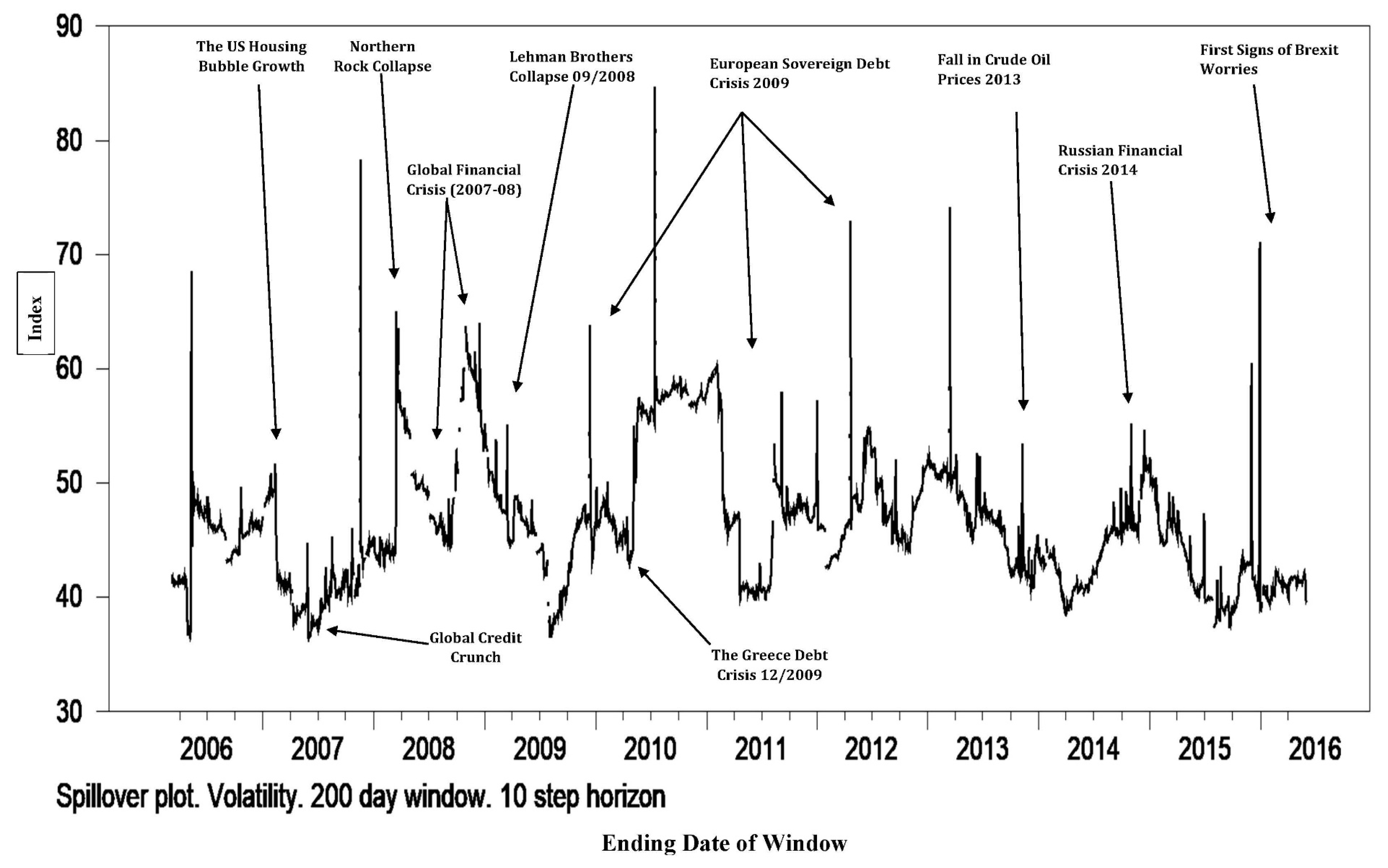
To examine the data, the spillover index described above allows the aggregation degree of cross-market spillovers across the large data, which consist of 2872 samples into a single spillover measure. We use second-order 23 variables with 10-step-ahead forecasts.
Table 3 and
Table 4 show the results of return spillover and volatility spillover, respectively.
4.2. Net Spillovers
To generate the net volatility spillovers, we follow (
Diebold and Yilmaz 2012) by first calculating the directional spillovers, which can be achieved by normalising the elements of the generalised variance decomposition matrix. This way, we can measure the directional volatility spillovers received by (developing) countries from the developed countries or vice versa as follows:
Thus, from the above equation, the net volatility spillovers can be obtained from market
i to all other markets
j as follows:
4.3. Net Pairwise Spillovers
Given the net volatility spillovers described in Equation (12), which provides the net volatility of each market contribution to others, then, it is relatively easy to examine the net pairwise volatility as follows:
Similarly, the net pairwise volatility spillover between markets i and j is represented by the difference between the gross volatility shocks communicated from market i to market j included those communicated from j to i.
4.4. ARCH Model
The basic autoregressive conditional heteroscedasticity (ARCH) model is constructed from two equations (a mean equation and a variance equation). The mean equation defines the behaviour of the time series data mean, therefore, the mean equation is the linear regression function, which contains constant and other explanatory variables. In the following equation, the mean function only contains an intercept:
Considering Equation (16), the time series is expected to vary about its mean (
randomly. In this case, the error of the regression is distributed normally and heteroskedastic. The variance of the current error period depends on the information that is revealed in the proceeding period
Poon (
2005). However, the variance equation defines the error variance behaviour where the variance
is given the symbol
as follows:
It is clear from Equation (17) that
depends on the squared error in the proceeding time period
Bollerslev et al. (
1994). Additionally, in the same equation, the parameters have to be positive to ensure the variance
, is positive. In addition, the large multiplier (LM) test can also be used to examine the presence of ARCH effects in the data, (i.e., whether α > 0). However, to carry out this test, we estimate the mean equation, then save and square the estimated residuals,
.
Table 5 shows the regression result of the squared residuals. Then, for the first order ARCH model, we regress
on the lagged residuals
and the following constant:
where
vt represents the random term. The null and alternative hypothesis are:
Table 6 shows the result of the large multiplier (LM) test, which confirms the presence of ARCH in the data. Therefore, the forecasted error variance is an in-sample prediction model essentially based on an estimated variance function as follows:
And the forecast error variance , demonstrates the time period of our sample (2005–2016).
6. Time-Varying Volatility Spillovers
In this section, we present the results of the time-varying volatility spillovers among developed and developing countries using autoregressive conditional heteroskedasticity (ARCH). Time-varying volatility helps to investigate sources of significant shifts in the volatility during the time period of our sample (2005–2016). This is because an ARCH model is designed to capture persistence in time-varying volatility based on squared returns
Poon (
2005). The ARCH model has a unique structure, where ”autoregressive” means high volatility tends to persist, ”conditional” refers to time-varying or specific point on time, and ”heteroskedasticity” refers to non-constant volatility
Poon (
2005). Before applying the ARCH (1) model, we first generate the squared residuals using regression, which contains only an intercept.
Table 5 shows the regression result of the squared residuals. This is because the squared residuals ensure that the conditional variance is positive and, consequently, the leverage effects cannot be captured by the ARCH model
Engle (
2001b).
Table 5.
Regression results (squared residuals).
Table 5.
Regression results (squared residuals).
| Variable | | p-Value |
|---|
| Ehat2 | 8.12 | 0.000 |
| No-of-Obs: 2.871 R-Squared: 0.022 Adj R-Squared: 0.002 MSE: 1.3 × 10⁻⁷ |
Second, we test the data for the presence of ARCH effects using the Box–Pierce large multiplier (LM), which provides the most appropriate results
Alexander (
2002).
Table 6 displays the result of the large multiplier’s (LM) test for the presence of ARCH effects in the data.
Table 6.
LM test results for autoregressive conditional heteroskedasticity (ARCH).
Table 6.
LM test results for autoregressive conditional heteroskedasticity (ARCH).
| lags(p) | chi2 | df | Prob > chi2 |
|---|
| 1 | 1 | 64.443 | 0.0000 |
The LM results show the null and alternative hypotheses, the statistic and its distribution, and the
p-value, which indicates the presence of ARCH (p) model disturbance in the data. Thus, we estimate the ARCH (1) model and generate the forecast error variance, which is essentially an in-sample prediction model based on the estimated variance function (see Equation (19) for more details).
Table 7 shows the result of the conditional variance of the estimated ARCH (1) model. The conditional variance in the ARCH model is allowed to change over time as a function of past error leaving the unconditional variance constant
Bollerslev (
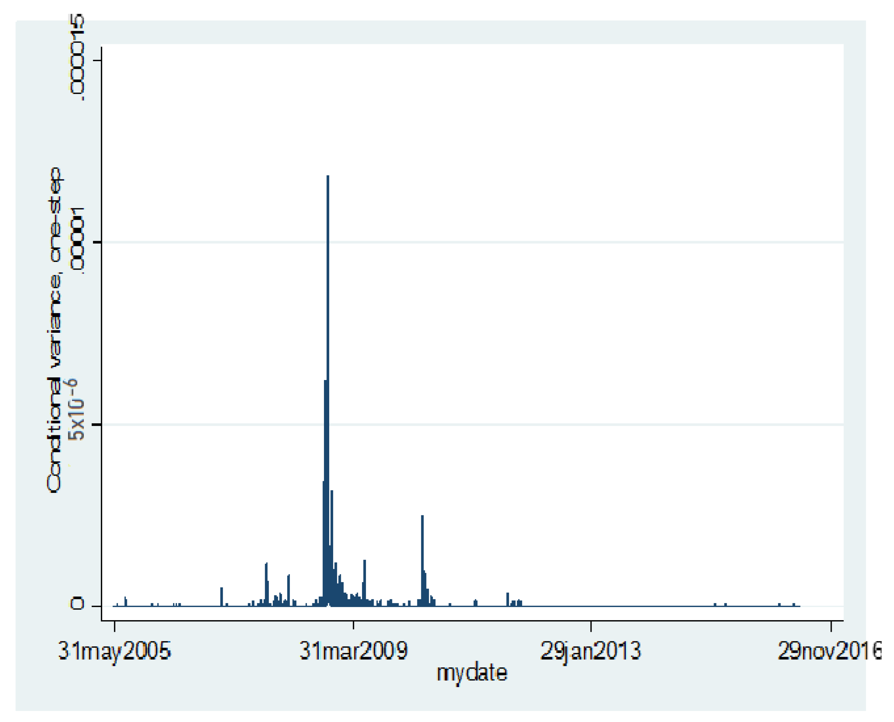
1986). Then, we proceed by plotting the forecast error variance against the time period of our sample (2005–2016).
Figure 5 shows the result of the ARCH (1) model, which implies that the volatility spillovers from developed countries to the developing countries seem to be specifically strong in 2008.
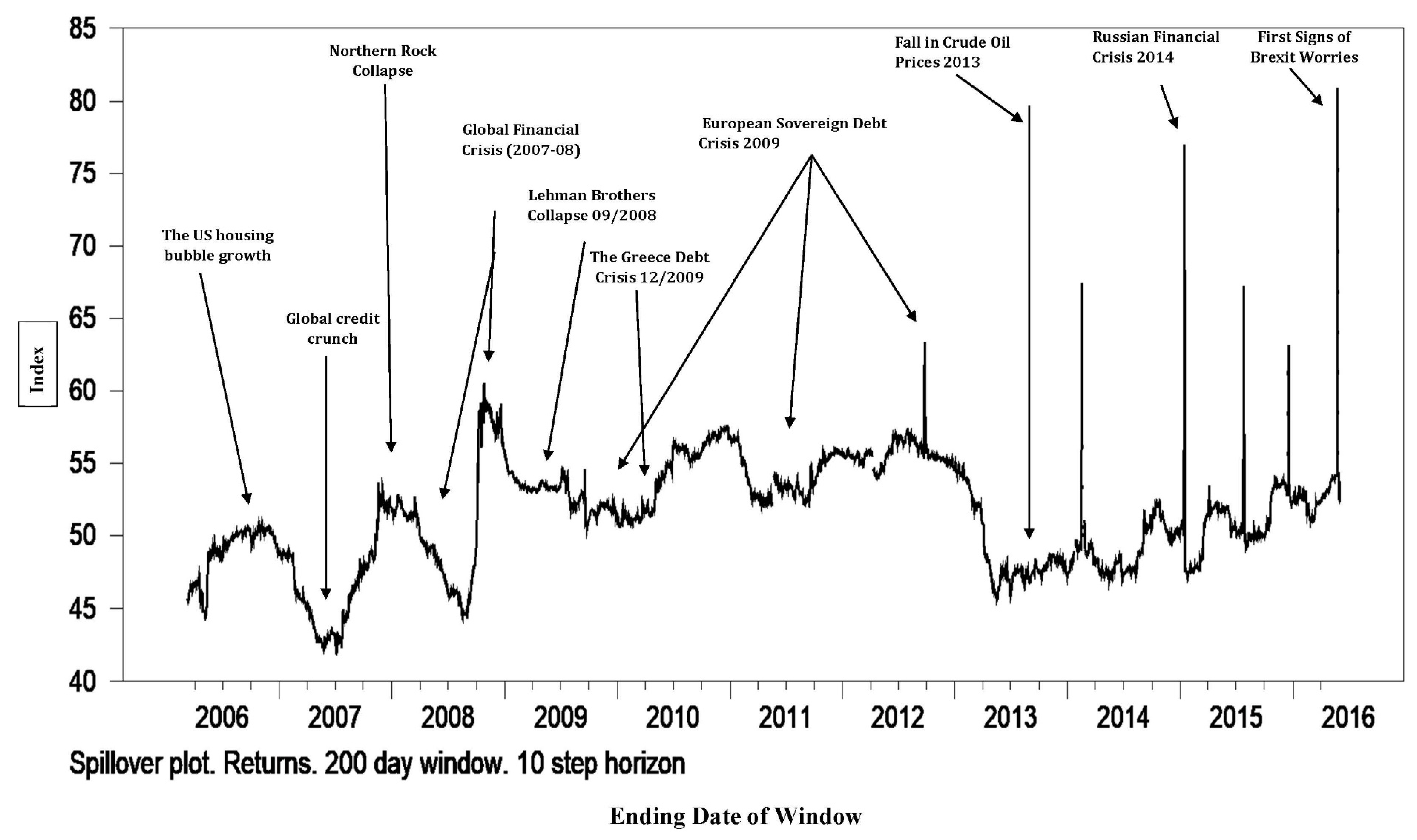
Thus, the result indicates that the foreign exchange markets’ channels between developed and developing countries exhibit time-varying persistence in its conditional volatilities over the crisis period. This result is consistent with the spillover index findings of both the static analysis (
Table 4) and the dynamic analysis (
Figure 2 and
Figure 4). It also shows that all the currencies in the sample from both (developed and developing) countries are characterised by clustering volatility. Our findings indicate that the global foreign exchange market experiences somewhat relatively sedate volatility spillovers from 2005 to 2007. Then, the foreign exchange market’s volatility spillovers become much more volatile in 2008–2009. These results are consistent with the dynamic analysis of the spillover indices (
Figure 2), which captured the 2008/2009 financial crisis.
7. Net Spillovers and Net Pairwise Volatility Spillovers
In this section, we present the results of the net spillovers and the net pairwise spillovers between developed and developing countries over the time period of our sample (2005–2016). The key features of the net volatility spillovers show the difference between the gross volatility shocks that are transmitted to and those received from all other markets (
Diebold and Yilmaz 2012). Therefore, the net pairwise volatility spillover (Equation (14)) between country
i and
j is the difference between the gross volatility shocks transmitted from a country i to country
j including the transmission from
j to
i (
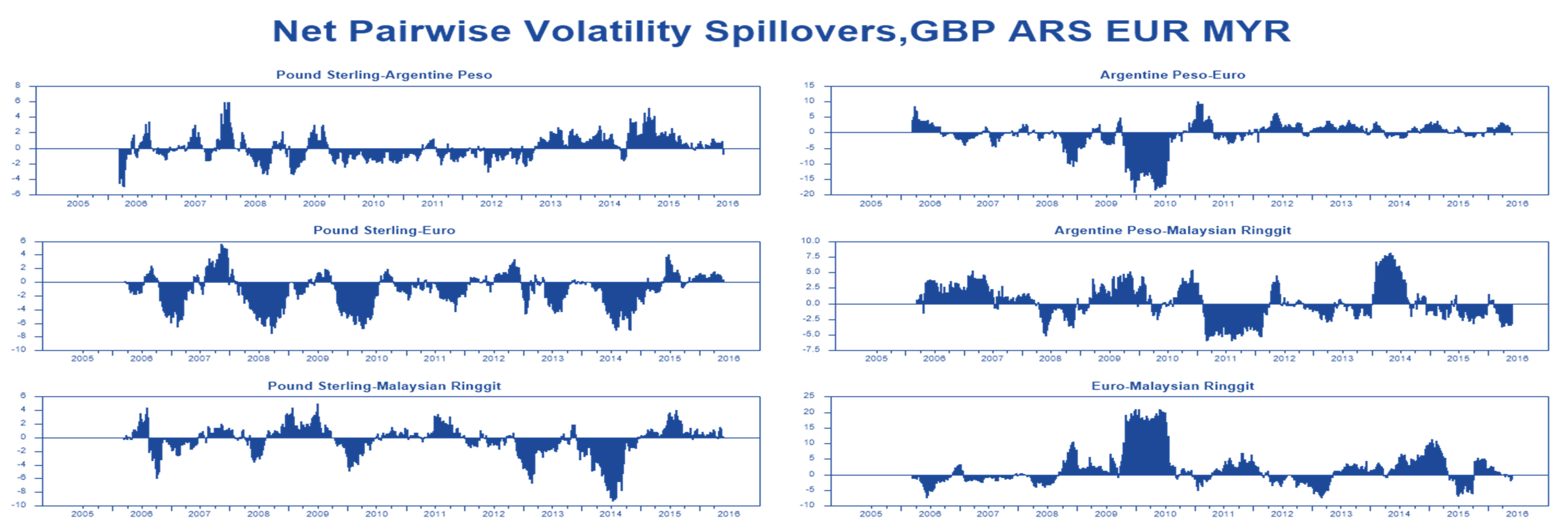
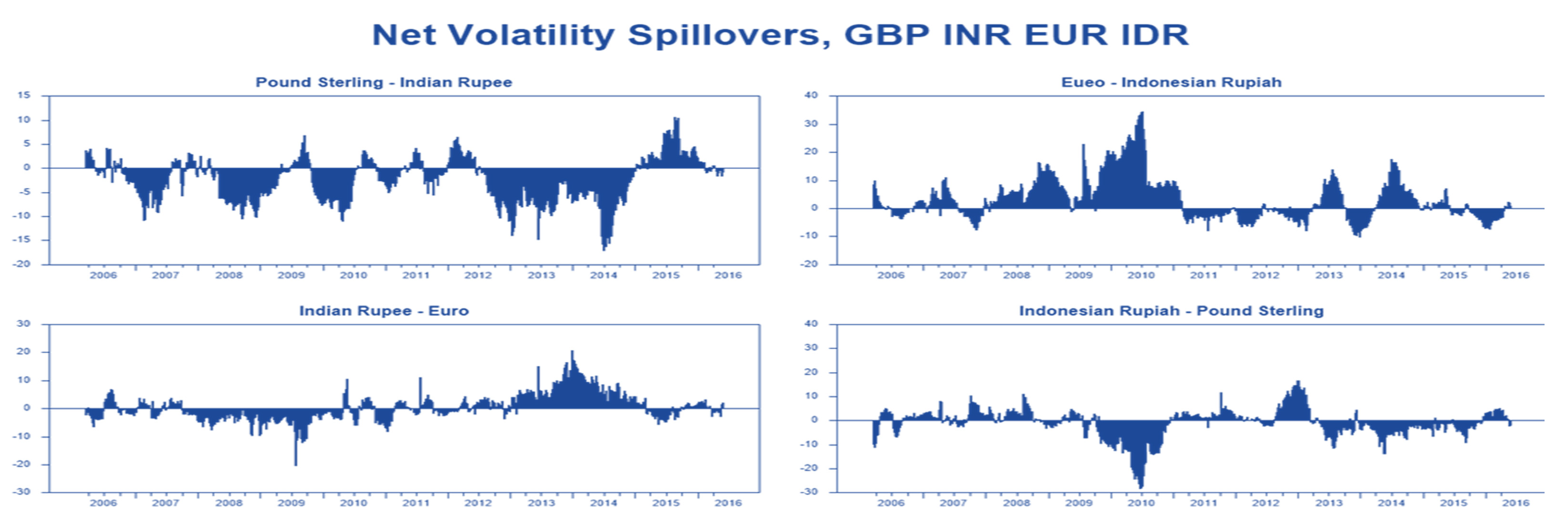
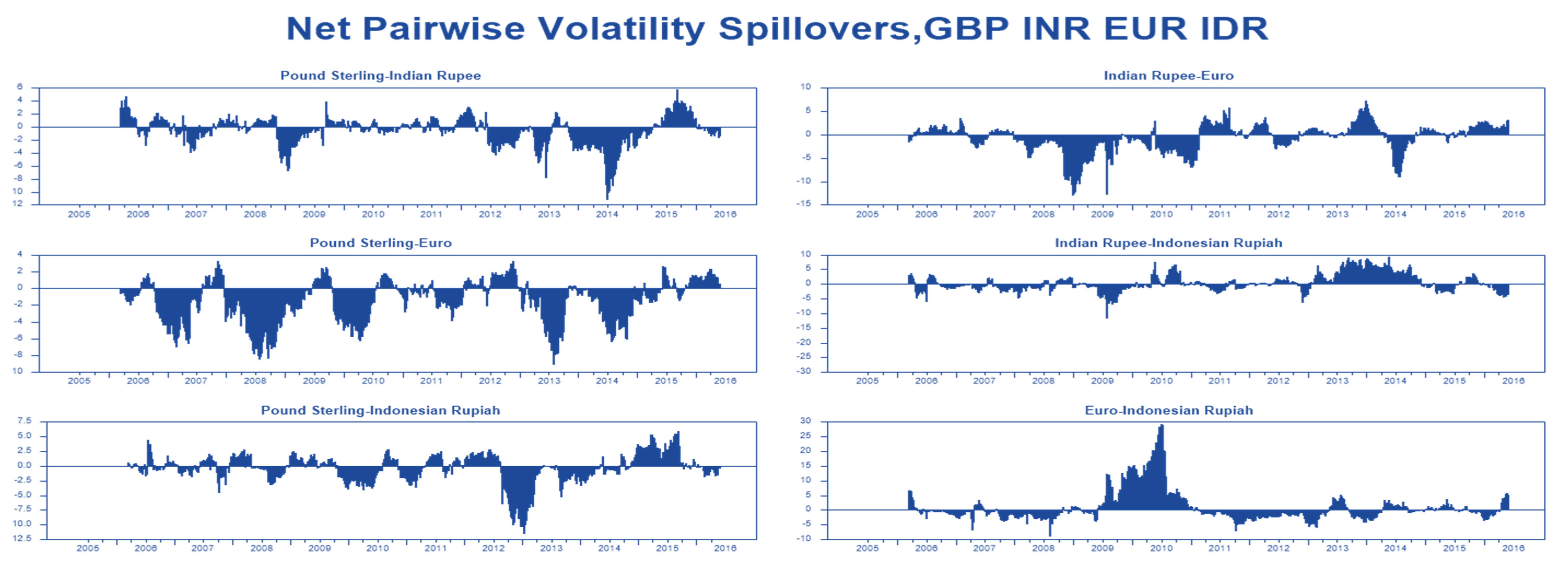
Diebold and Yilmaz 2012). As shown in Equation (12), the net volatility spillovers offer important information about the amount of volatility in net terms that each country contributes to other countries. Therefore, the main focus point of this section is to calculate the net volatility and the net pairwise volatility spillovers between developed and developing countries. Due to a large number of countries (23) in our sample, only 16 currencies were selected, which we present in
Figure 6,
Figure 7,
Figure 8 and
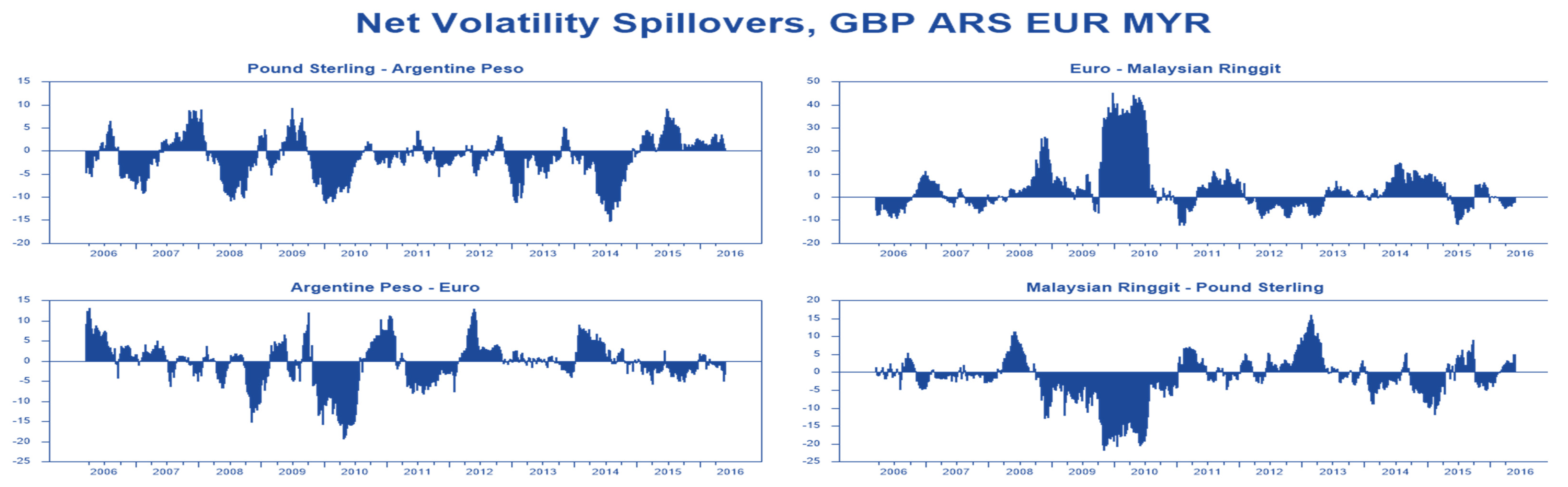
Figure 9.
During the time period of our sample (2005–2016), there were two major events of net volatility spillovers through the global foreign exchange market, in particular, during the 2008/2009 financial crisis and the European sovereign debt crisis in 2009/2013. However, before the recent financial crisis and the European sovereign debt crisis, the net volatility spillovers between developed and developing countries was relatively low; however, things changed drastically after 2007, when the net volatility spillover from the EUR to the Malaysian ringgit (
Figure 8) jumped to 20% in the third quarter of 2008 and 40% in the third quarter of 2009. These results are consistent with the time-varying volatility results, which imply that the foreign exchange market experienced low volatility from 2005 to 2007. The pound sterling (GBP) and the Euro (EUR) (
Figure 6,
Figure 7,
Figure 8 and
Figure 9) both act as giving and receiving of the net volatility transmissions, with almost similar magnitudes across the global foreign exchange markets. This finding supports the static analysis of the spillover index (
Table 4) that the pound sterling (GBP) and the Euro (EUR) are the main contributors of volatility spillovers.
The Indonesian rupiah (IDR) also receives a significant amount of volatility spillovers from the Euro (EUR) (
Figure 7), especially during the recent financial crisis and the European sovereign debt crisis in 2009/1013. In addition, the Euro (EUR) receives a large amount of volatility spillovers from the Malaysian ringgit (
Figure 9), which indicates that developed countries act as receivers and transmitters of volatility spillovers. The Argentine peso (ARS) contributes as well as receives a significant amount of volatility from the Malaysian ringgit (MYR),
Figure 9. The net volatility spillover from the pound sterling (GBP) to the Euro (EUR) (
Figure 9) seems relatively low while receiving a significant amount of volatility spillover from the Euro (EUR). The fact that the pound sterling (GBP) contributes as well as receives a large amount of volatility spillover from the Euro (EUR) shows the increased link between developed countries in the global foreign exchange market.
8. Conclusions
The critical question is whether the effects of return and volatility spillovers are bidirectional between developed and developing countries. Thus, in this paper, we examined the impact of return and volatility spillovers on global foreign exchange markets across developed and developing countries. Quoted against the US dollar, the data sample was comprised of twenty-three global currencies across developed and developing countries. Seven of the currencies are the most actively traded globally, including the British pound sterling (GBP), the Euro (EUR), the Australian dollar (AUD), the Swiss franc (CHF), the Icelandic krona (ISK), the Czech Republic koruna (CZK), and the Hong Kong dollar (HKD). We discussed the effect of return and volatility spillovers between developed and developing countries, using the generalised vector autoregressive (VAR) methodology. We provided the empirical results of the spillover index, in the form of a static analysis of “the spillover tables”, as well as a dynamic analysis in the form of “spillover plots”. We also discussed the time-varying volatility spillovers among developed and developing countries using autoregressive conditional heteroskedasticity (ARCH).
During the time period of the sample investigation (2005–2016), several exciting economic events reveal the magnitude and extent of the volatility spillovers’ effect across global foreign exchange markets, in particular, from the perspective of the recent financial markets’ interconnectedness. Nevertheless, the findings did not disclose evidence of bidirectional spillovers between developed and developing countries. However, we found non-negligible evidence of unidirectional spillovers (
Table 4) from developed to developing countries. We also found that developed countries acted as receivers and transmitters of volatility, dominated by the British pound sterling (GBP), Australian dollar (AUD), and the Euro (EUR), whereas developing countries were net receivers of volatility.
Furthermore, the empirical results conclusively show that the magnitude and extent of the return and volatility spillovers were significantly large within the European region (Eurozone and non-Eurozone currencies), in particular, during crisis episodes, whereby the volatility spillovers replicate remarkable bursts.
This phenomenon is in line with the findings presented by
Glick and Rose (
1998) and
Yarovaya et al. (
2016) that currency crises tend to be regional. From a policy point of view, in this paper, we document significant macroeconomic implications. Firstly, the extent of global foreign exchange markets’ volatility channels highlight the significance of contagion and systemic risk, particularly from the global systemically important financial institutions. Secondly, the substantial return spillovers between developed countries, especially within the European region (Eurozone and non-Eurozone currencies), further quantify the importance of cross-market linkages and the recent financial innovations. In addition, it opens avenues for a better understanding of the potential crisis of a highly interlinked nature, mirrored in the historical economic events.
Overall, this paper contributes to the literature of intra-foreign exchange markets’ channels from the perspective of developed and developing countries. Here, the empirical results show that the spillover channels between developed and developing countries are insignificant. However, this raises the question of how the recent financial turmoil (which affected both developed and developing countries) propagated across the global economies.


