Article

Financial Crises, Macroeconomic Variables, and Long-Run Risk: An Econometric Analysis of Stock Returns Correlations (2000 to 2019)

Department of Economics, School of Social Sciences, University of Genoa, Via Vivaldi 5, 16126 Genoa, Italy
J. Risk Financial Manag. 2021, 14(3), 127; https://doi.org/10.3390/jrfm14030127
Submission received: 13 January 2021 / Revised: 18 February 2021 / Accepted: 25 February 2021 / Published: 17 March 2021
(This article belongs to the Special Issue Co-movement of International Financial Markets)

Abstract

:
This paper focuses on four major aggregate stock price indexes (SP 500, Stock Europe 600, Nikkei 225, Shanghai Composite) and two “safe-haven” assets (Gold, Swiss Franc), and explores their return co-movements during the last two decades. Significant contagion effects on stock markets are documented during almost all financial crises; moreover, in line with the recent literature, the defensive role of gold and the Swiss Franc in asset portfolios is highlighted. Focusing on a new set of macroeconomic and financial series, a significant impact of these variables on stock returns correlations is found, notably in the case of the world equity risk premium. Finally, long-run risks are detected in all asset portfolios including the Chinese stock market index. Overall, this empirical evidence is of interest for researchers, financial risk managers and policy makers.

1. Introduction

A large body of empirical literature documents the time-varying nature of asset returns co-movements.
Focusing on stock returns, this literature relies on various econometric techniques ranging from wavelet correlation analysis (Dajcman et al. 2012), to a quantile regression approach (Ciner et al. 2013) and, more extensively, to alternative specifications of Engle’s (2002) dynamic conditional correlation (DCC) model. This last strand of work has implemented, among others, the standard version of the DCC model (Syllignakis and Kouretas 2011), the asymmetric version (Gjika and Horvath 2013), the Fractionally Integrated Asymmetric Power ARCH specification (Dimitriou et al. 2013), and the DCC-Mixed Data Sampling specification to extract short- and long-run correlations components (originally introduced by Colacito et al. (2011)).
Notwithstanding the overwhelming evidence supporting the time-varying nature of stock returns correlations and the use of powerful econometric techniques, the empirical analysis of these co-movements still displays some significant drawbacks with reference to the following issues:
(a)
The impact of financial crises on stock returns co-movements;
(b)
The impact of macroeconomic and financial variables on stock returns correlations;
(c)
The relationship between conditional correlations and conditional volatilities of the corresponding stock markets.
A major limitation of the literature exploring the effects of financial crises is the absence of a comprehensive approach as regards stock market indexes and the set of crises included in the empirical investigation. Earlier contributions focus exclusively on some major Asian countries (Yang 2005), on Central Europe stock markets (Syllignakis and Kouretas 2011; Gjika and Horvath 2013), or on BRICS and Asian stock market indexes (Hwang et al. 2013). The focus of more recent research shifts instead to US and European aggregate stock market indexes (Dimitriou and Simos 2014) or to stock market indexes of a large number of European countries (Nitoi and Pochea 2019). However, even these more recent contributions do not analyze the effects of financial crises occurring after the 2010–2012 Eurozone debt crisis.
An analogous drawback characterizes applied work exploring the determinants of stock returns co-movements (see point (b) above). Syllignakis and Kouretas (2011) use some macro-variables proxying the degree of business cycle convergence, monetary policy convergence, and inflationary convergence between Central and Eastern European economies and Germany. Although the choice of these variables reflects the main issues addressed in the paper, this set of macro-variables is highly restricted. The use of the Sovereign CDS spread, the TED spread and the VIX volatility index is quite common in subsequent work focusing on dynamic correlations between emerging economies and US stock market returns (Hwang et al. 2013; Cai et al. 2016). While this variable selection approach is more inclusive, other important financial variables, such as the world equity risk premium or the European Central Bank (ECB) systemic stress composite indicator, have been neglected in the literature. Moreover, although some recent work accounts for the influence of economic integration and institutional macro-variables (e.g., Nitoi and Pochea 2019), the role of consumer confidence or economic policy uncertainty indicators has never been explored, to the best of my knowledge. Yet, these indicators could potentially have a strong impact on dynamic returns co-movements on international stock markets.
Turning to point (c) above, the relationship between conditional correlations and conditional volatilities is important to understand whether the benefits from portfolio diversification during turbulent periods. This information is crucial in many standard financial activities, such as risk management or option pricing. If stock market linkages are higher when the level of risk increases (i.e., if we observe a positive relationship), long-run risks are greater than they appear in the short run, and portfolio defensive strategies will become more expensive than previously anticipated (Cappiello et al. 2006). Overall, the available evidence supports the existence of a positive relationship between correlations among stock returns and their volatilities: see, among others, Yang (2005), Cai et al. (2009), Syllignakis and Kouretas (2011), and Gjika and Horvath (2013). Cappiello et al. (2006) provide an in-depth empirical analysis using worldwide data for many industrial countries, and document dramatic increases in conditional equity correlation series among regional groups during periods of financial turmoil; they also document that, on average, this phenomenon is stronger for equities than for bonds.
This paper provides an econometric analysis of stock returns correlations using data for the last two decades. I focus on some major equity price indexes that are highly relevant in the portfolio allocation choices of a typical international investor, and include all the most important economic areas ranging from US (SP 500), to Europe (Eurostock 600), Japan (Nikkei 225), and China (Shanghai composite index).
Consistently with the previous discussion, I contribute to the existing literature in three main directions.
First, differently from current applied work, I provide a comprehensive analysis about the effects of all financial crises occurred over the last two decades. While the set of financial turmoil episodes addressed in existing studies is confined to the global financial crisis (2007/2009) and to the Eurozone debt crisis (2010/2012), this investigation extends up to more recent years, allowing to explore the effects of the latest financial crises on stock returns correlations.
Second, I focus on a wide range of macroeconomic and financial variables, neglected in the existing literature, and potentially exerting a strong influence on returns co-movements. As regards financial variables, I consider two outstanding financial indicators proxying, respectively, the overall degree of risk aversion (world equity risk premium) and the degree of financial system stress (ECB—composite indicator of systemic stress). Moreover, as regards macroeconomic variables, I consider some economic policy uncertainty and consumer confidence indicators whose influence on assets co-movements should primarily depend on emotional reactions of economic agents.
A third contribution is related to the connections between conditional correlations and conditional volatilities, where I do not exclusively focus on stock returns co-movements, but also explore the impact of conditional volatilities on bilateral correlations between equities and “safe-haven” assets.
The paper outline is as follows. The next section describes the data set, provides some descriptive statistics, and discusses maximum-likelihood estimates from Engle’s (2002) dynamic conditional correlation (DCC) model. Section 3 is devoted to the econometric analysis of dynamic conditional correlations. I start by analyzing the impact of financial crises on stock returns correlations (Section 3.1), and then focus on the impact of macroeconomic and financial variables (Section 3.2) and of conditional volatilities (Section 3.3). Section 4 concludes.

2. Data, Descriptive Statistics and Parameters Estimates from Engle (2002) DCC Model

2.1. Data and Descriptive Statistics

The analysis relies on monthly data from January 1999 to March 2019, yielding a total of 243 observations. This frequency helps to increase the speed of the estimation process, since one purpose of this paper is to explore the impact of a set of macroeconomic and financial variables (available at a monthly frequency) on stock returns correlations. However, as pointed out by one referee, alternative research options are available resorting to a Garch mixed data sampling (Garch–MIDAS) approach. Some interesting examples of this approach in a univariate setting are provided in Engle et al. (2013) and Amendola et al. (2019). Engle et al. (2013) revisit the relationship between US stock returns and volatility over a long time horizon covering more than one century. Amendola et al. (2019) extend the standard Garch–MIDAS model to account for the asymmetric impact of macro-variables on stock market volatility, showing that the proposed specification yields better volatility forecasts and significant utility gains to a representative investor. Colacito et al. (2011) extend this framework to a multivariate set of asset returns in the context of Engle’s (2002) DCC model, documenting the superior fit of this class of dynamic correlations models. A DCC–MIDAS model along these lines represents, therefore, a natural extension of the present research, as underlined in the concluding section. I am grateful to an anonymous referee for drawing my attention on this class of models, allowing to directly evaluate the impact of macroeconomic variables on dynamic correlations.
I consider four major aggregate stock price indexes, namely: the SP 500, the Stock Europe 600, the Nikkei 225 and the Shanghai composite price index. Moreover, I also include two important “safe-haven” assets, namely gold and the Swiss Franc/US Dollar nominal exchange rate. These latter variables are recognized as typical “safe-haven” assets in the financial literature (see Hood and Malik (2013) as regards gold’s hedging properties, and Ranaldo and Söderlind (2010) as regards the Swiss Franc). All data are from Thomson Reuters/Datastream and refer to end-of-month values (The relevant references and Thomson Reuters codes are the following: SP 500 Composite Price Index: Thomson Reuters code “S&PCOMP”; Stock Europe 600 Price Index: Thomson Reuters code “DJSTOXX”; Nikkei 225 Stock Average: Thomson Reuters code “JAPDOWA”; Shanghai SE Composite Price Index: Thomson Reuters code “CHSCOMP”; Gold: Gold Bullion LBM $/t oz; Thomson Reuters code: “GOLDBLN”; Swiss Franc: Swiss Franc/U$ Exchange Rate; Thomson Reuters code: “TDCHFSP”).
The econometric model relies on monthly returns of these series, computed by taking their first differences expressed in natural logs.
Descriptive statistics for these asset returns are reported in Table 1.
All average returns are close to zero, in line with the efficient market hypothesis. Moreover, none of them is statistically significant, with the exception of gold returns which display a modest positive average return during the sample period.
As shown by standard deviations, all return series exhibit a great deal of variation. Focusing on stock market indexes, the variability of the Shanghai composite returns is higher, whereas the remaining stock markets display lower values around four to five percent. In line with the recent literature (see, e.g., Bedoui et al. 2018), the variability of gold returns is broadly similar to that of stock markets, whereas Swiss currency returns exhibit lower variability.
All series are negatively skewed, pointing out asymmetric distributions with long tails in the leftward direction. Moreover, all returns display positive excess kurtosis, pointing out fatter tails relative to the normal distribution. Consistently with these results, the Jarque–Bera test strongly rejects the null of normality for all returns.
Arch tests at lags 1 and 6 almost always reject the null of homoscedasticity, implying that a multivariate Garch approach is an appropriate econometric framework to model conditional volatilities. The Ljiung–Box test, while showing some evidence of first-order serial correlation (Eurostock 600, Nikkei 225, Shanghai composite), supports the absence of serial correlation at higher lags for all asset returns (with the Shanghai composite as the only relevant exception).
Table 2 contains the unconditional correlation coefficients. Since the exchange rate series is defined as the number of Swiss Francs per one unit of US dollars, a decrease (increase) in the log-difference of this series corresponds to an increase (decrease) in Swiss Franc returns. Therefore, in bilateral correlations involving Swiss Franc returns (DS), a positive (negative) correlation coefficient indicates a negative (positive) correlation with other asset returns).
All correlations involving “safe-haven” assets are almost equal to zero and not statistically significant according to the Pesaran and Timmermann (1992) nonparametric test. This result reiterates the role of gold and the Swiss Franc as important “safe-haven” assets, as they are uncorrelated with traditional financial assets. The correlation between gold and the Swiss Franc is relatively high, positive, and statistically significant. Although lower than positive correlations values recorded between gold and other precious metals (see, e.g., Sensoy 2013), this result confirms the existence of positive long-run co-movements between “safe-haven” assets, potentially reducing the diversification benefits across them.
Unconditional correlations between stock returns (Table 2, first four rows) are positive and statistically significant, documenting relevant co-movements between major stock markets. The highest values are obtained for bilateral correlations among US, European and Japan stock markets, whereas those involving the Chinese stock market are positive but notably lower. This last result may be ascribed to the lower degree of financial integration of the Chinese economy.
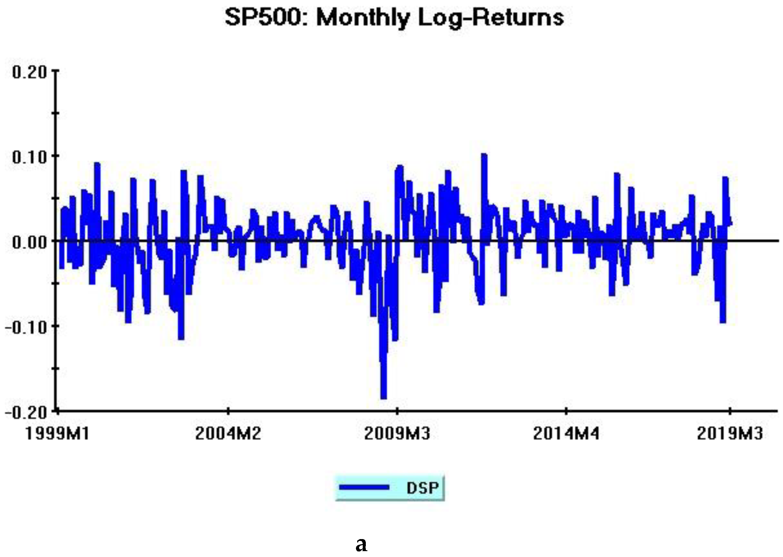
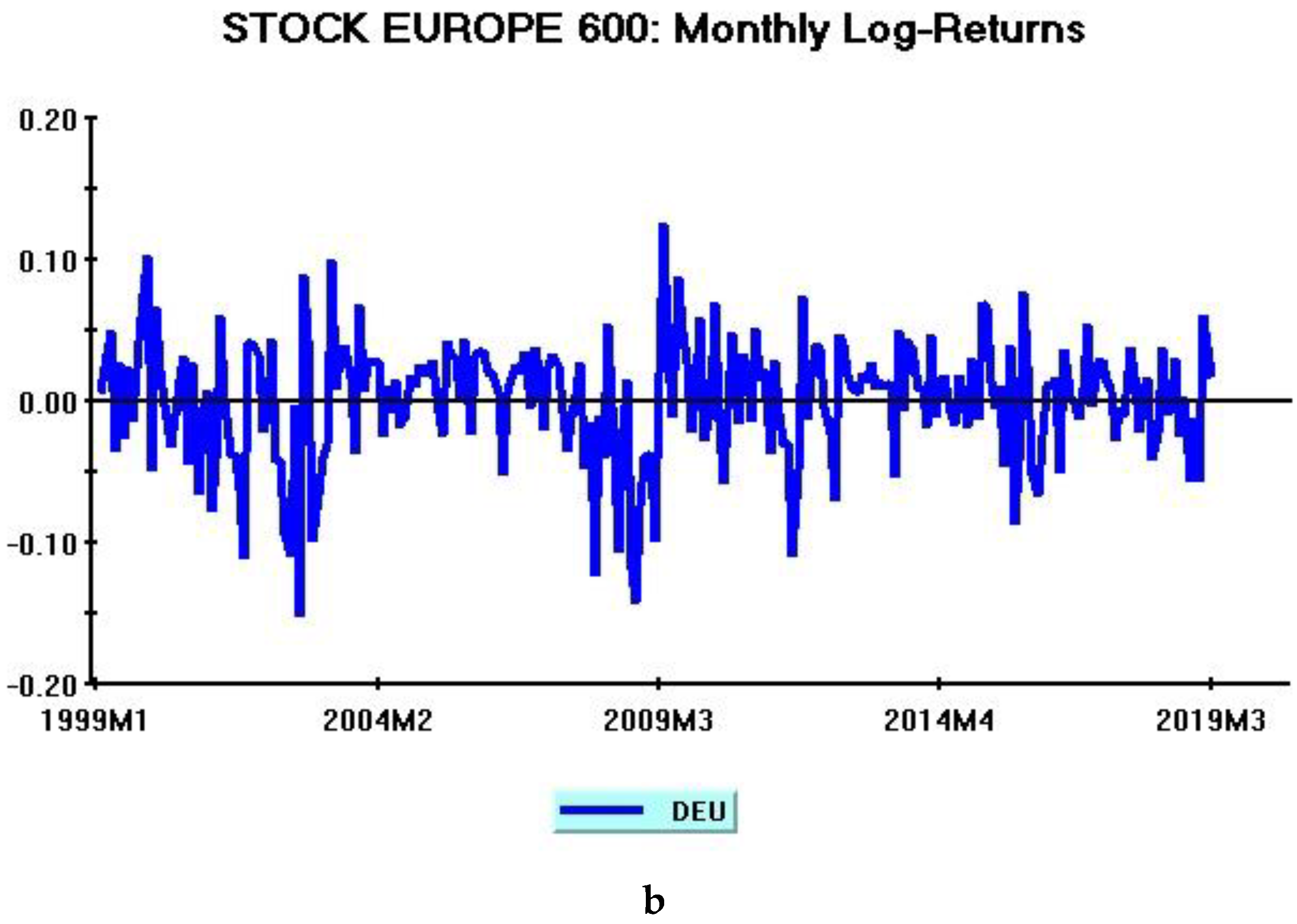
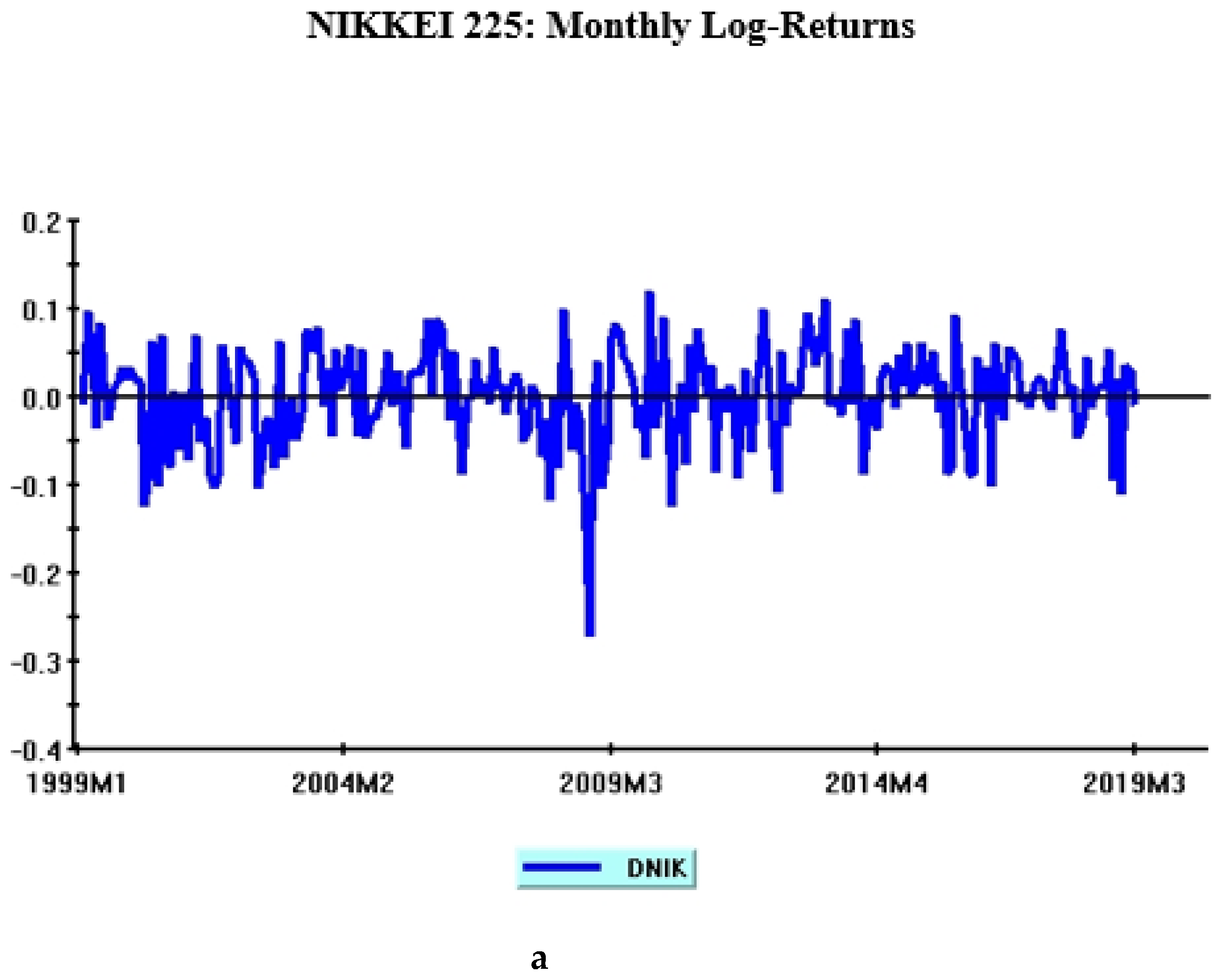
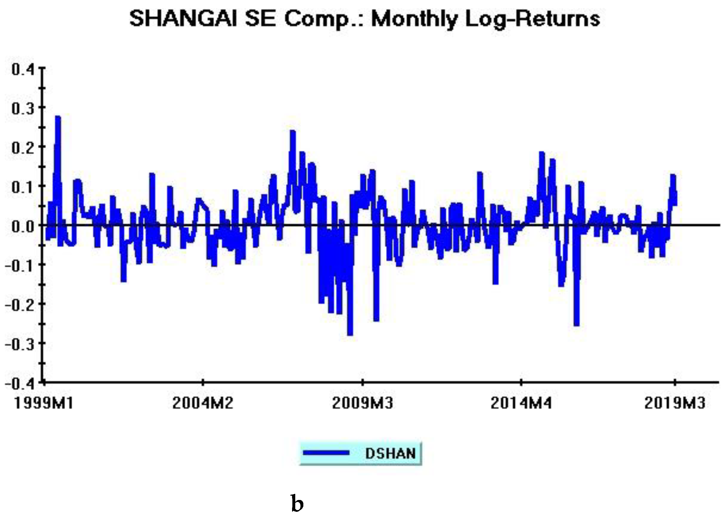
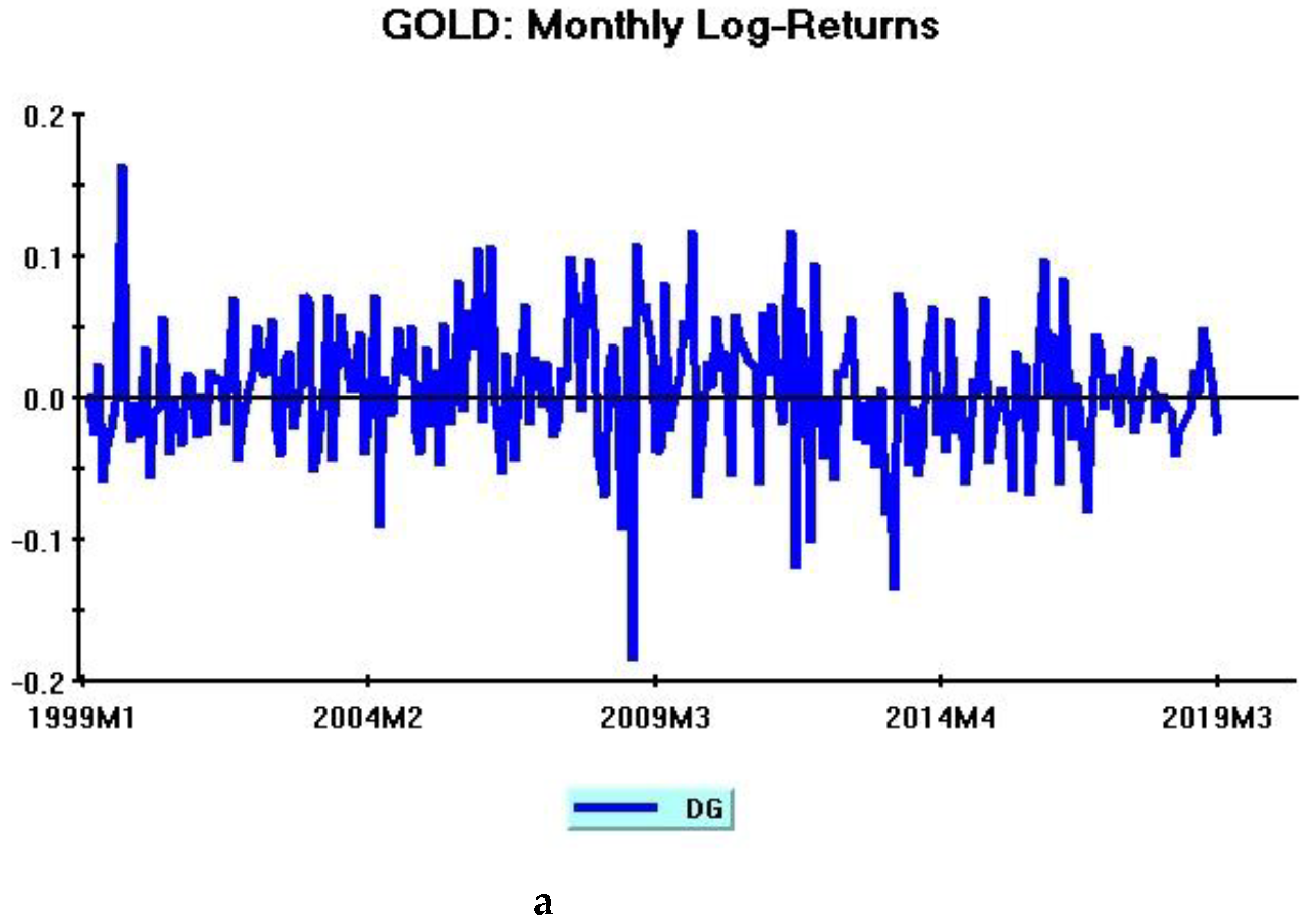
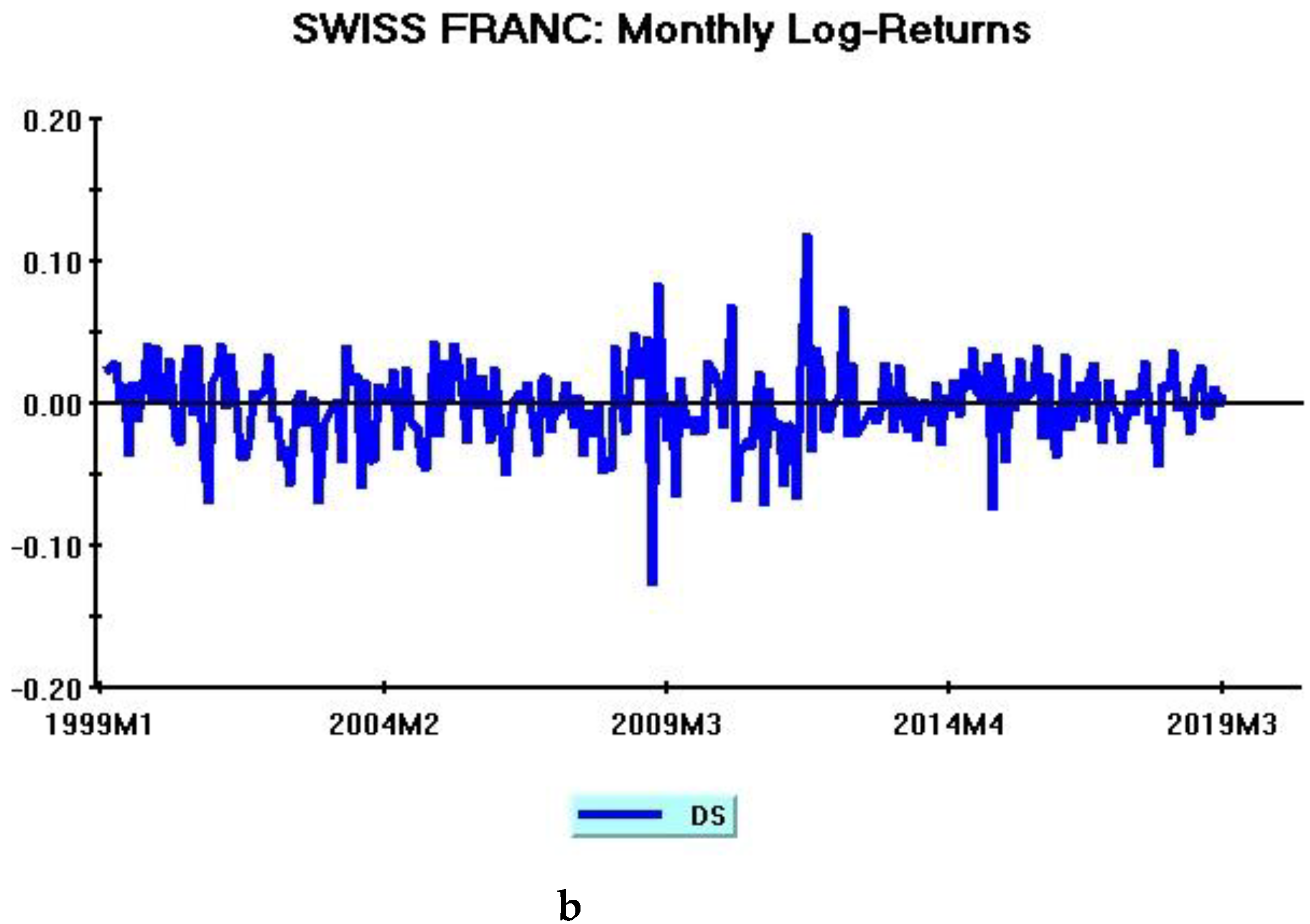
Figure 1, Figure 2 and Figure 3 display financial assets monthly returns.
These series exhibit volatility clustering, a typical feature of financial data, with returns dynamics alternating between high and low volatility phases. Overall, this feature is more evident for stock market returns.
Large volatility swings are observed along the beginning of the sample, corresponding to the end of the dot-com bubble and the months subsequent to the September 2001 terrorist attack. This turbulent initial phase is followed by a low-volatility regime for most return series extending from 2004 to 2007. The central part of the sample, including the global financial crisis (2008 to 2009) and the Eurozone debt crisis (2010 to 2012) displays the most unstable volatility patterns, with large upward and downward swings involving all assets. During the last part of the sample, further volatility clustering episodes are apparent. After a relatively tranquil phase, a new high-volatility regime is observed from the last quarter of 2014 to the end of 2015 (including both the Russian financial crisis and the Chinese stock market crisis).

2.2. Parameters Estimates and Pairwise Correlation Patterns

The econometric analysis of financial assets correlations requires, as a preliminary step, the computation of dynamic conditional correlations between all return series.
An efficient econometric framework is the dynamic conditional correlation (DCC) model proposed in Engle’s (2002) seminal contribution, which belongs to the class of multivariate Garch models. The main advantages of Engle’s (2002) approach are that it relies on a two-step estimation procedure providing consistent estimates of the conditional correlation matrix, and that it allows a multivariate analysis of asset returns in a parsimonious parameters setting.
Let rt (r1t, ……, rnt) represent an (n × 1) vector of financial asset returns at time (t). Moreover, let εt1t,……, εnt) be a (n × 1) vector of error terms obtained from an estimated system of mean equations for these series.
Engle (2002) proposes the following decomposition for the conditional variance–covariance matrix of asset returns:
Ht = DtRtDt
where Dt is a (n × n) diagonal matrix of time-varying standard deviations from univariate Garch models, and Rt is a (n × n) time-varying correlation matrix of asset returns (ρij,t).
The conditional variance–covariance matrix (Ht) is estimated in two steps. In the first step, univariate Garch (1, 1) models are applied to mean returns equations, thus obtaining the conditional variance estimates for each financial asset (σ2it; for i = 1, 2, ……, n), namely:
σ 2 it = σ ¯ 2 it ( 1 λ 1 i λ 2 i ) + λ 1 i σ 2 i , t 1 + λ 2 i ε 2 i , t 1
where σ ¯ 2it is the unconditional variance of the ith asset return, λ1i is the volatility persistence parameter, and λ2i is the parameter capturing the influence of past errors on the conditional variance.
In the second step, the residuals vector obtained from the mean equations system (εt) is divided by the corresponding estimated standard deviations, thus obtaining standardized residuals (i.e.,: uit = εit/ σ i , t 2 for i = 1, 2, ……, n), which are subsequently used to estimate the parameters governing the time-varying correlation matrix.
The dynamic conditional correlation matrix of asset returns may thus be expressed as:
Q t = ( 1 δ 1 δ 2 ) Q ¯   + δ 1 Q t 1 + δ 2 ( u t 1 ú t 1 )
where Q ¯ = E [ut út] is the (n × n) unconditional covariance matrix of standardized residuals, and δ1 and δ2 are parameters (capturing, respectively, the persistence in correlation dynamics and the impact of past shocks on current conditional correlations). One referee asked why the standard DCC model of Engle (2002) is used in place of the cDCC model of Aielli (2013). The cDCC model modifies the standard DCC model reformulating the correlation driving process (Equation (3)) as a linear multivariate Garch process. Simulation experiments carried out in Aielli (2013) for typical dynamic parameters values commonly observed in financial time series (i.e., δ1 + δ2 very close to 1, and δ2 ≤ 0.04) show that the correlation-fitting performance of these models is almost identical, with no apparent bias of the standard DCC estimator (see Aielli 2013, Section 4, and Figure 1, p. 284). Since the estimated values for the correlation process (δ1, δ2) match those mentioned in the above simulations, the use of the standard DCC model is appropriate in the present context. Extensions of this research using a larger number of financial series should instead rely on the cDCC model, which is a consistent large system estimator. This possibility is mentioned as a profitable research direction in the concluding section of this paper.
The Ljung–Box test displayed in Table 1 and further preliminary investigations reveal the presence of serial correlation in all returns series. For this reason, an AR(1) filter is applied to these series before proceeding with the estimate of the DCC model. Visual inspection of residuals from filtered series confirms that they are white noise processes.
The positive excess kurtosis values documented in Table 1 reveal that the distributions of asset returns display heavy tails and, in line with this empirical evidence, the Jarque and Bera (1980) statistics consistently reject the null hypothesis of normal distribution for monthly returns. This violation of the Gaussian assumption calls for a modification of Engle’s (2002) two-step estimation approach, combining the original DCC model with a multivariate t distribution in order to properly capture the fat-tailed nature of asset returns (Pesaran and Pesaran 2010). In line with these observations, the t-DCC specification of Engle’s (2002) seminal model developed by Pesaran and Pesaran (2010) is implemented in the present empirical investigation. Note that, under this alternative distributional assumption, Engle’s (2002) two-step original procedure is no longer applicable. The maximum likelihood estimator relies on a more efficient approach, involving the simultaneous estimation of the model’s parameters and an additional degrees-of-freedom parameter relative to the multivariate t distribution (see Pesaran and Pesaran 2010, Section 4 for technical details). The econometric software used in the present paper is Microfit 5.5 (see Pesaran and Pesaran 2009).
Conditional volatility coefficients (λ1, λ2) are unrestricted and assumed different for each financial asset (i) (see Equation (2)). A common correlation structure is instead imposed in the model’s estimation (see Equation (3)), while the correlation persistence parameter is restricted to 0.95 (δ1 = 0.95). This restriction on the δ1 parameter is needed in order to ensure convergence in the estimation algorithm.
The maximum likelihood estimator relies on 221 observations (20 observations are used to initialize the recursions) and converges after 34 iterations.
The validity of the estimated t-DCC model is assessed using the diagnostic tests suggested in Pesaran and Pesaran (2010). The null hypothesis of correct model specification is not rejected, at standard significance levels, neither by a Lagrange multiplier test for serial correlation in probability transform estimates nor by a Kolmogorov–Smirnov statistic testing the uniformity of the distribution of probability transform estimates. These testing procedures rely on a recursive computation of value-at-risk indicators. See Pesaran and Pesaran (2010), Section 5, for a technical discussion on conditional evaluation procedures based on probability integral transforms. Under the null hypothesis of correct model specification, probability transform estimates are serially uncorrelated and uniformly distributed in the interval (0, 1).
Table 3 contains the results from the Multivariate Garch t-DCC model.
The parameters relative to conditional variance equations are all positive and statistically significant, almost always at a 1% significance level. These results point out that all returns display significant time-variation in volatility dynamics, thus strongly supporting the choice of univariate Garch specifications. Garch coefficients (λ1i) are consistently higher than Arch coefficients (λ2i), thus pinpointing significant time dependencies in conditional volatilities. Moreover, the sums of estimated variance parameters (λ1i + λ2i) are always quite close to one, implying a high degree of persistence in conditional volatilities (particularly as regards Nikkei and Swiss Franc returns).
Turning to the coefficients describing the common correlation structure (δ1, δ2), this process appears mostly driven by lagged correlation dynamics, although past shocks also exert an appreciable effect, as witnessed by the δ2 parameter, which is significant at the 1% level. The high persistence in the correlation structure and the influence of past shocks on time-varying correlations are in line with most of the applied literature relying on a DCC approach to explore financial asset returns (see e.g., Pesaran and Pesaran (2010) as regards exchange rates, bonds and equities).
The estimated degrees-of-freedom parameter of the multivariate-t distribution (df) is equal to 10 and highly significant. This value is above that expected for a multivariate normal density, thus suggesting that this t-DCC model is well-suited to properly account for the heavier tails of error terms.
Overall, the evidence reported in Table 3 suggests that the estimated t-DCC model represents a reliable approach to explore asset returns co-movements.
While a detailed econometric analysis of these co-movements is postponed to Section 3, I conclude the present section providing some visual evidence about interesting features of these correlation patterns.
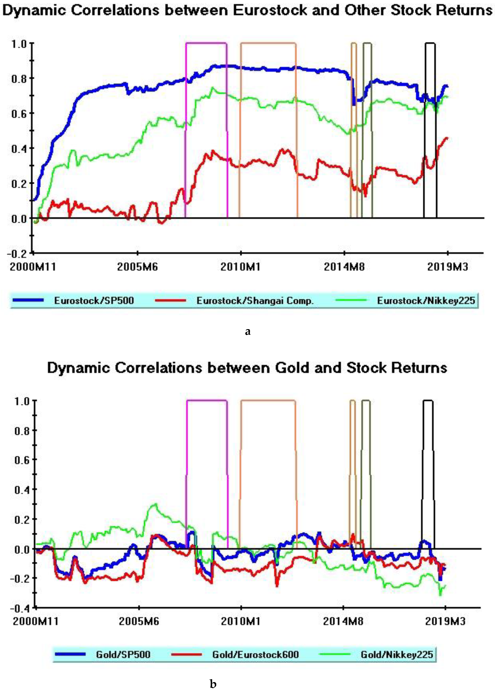
The upper section of Figure 4 shows time-varying correlations between Eurostock 600 and other stock returns indexes (SP 500, Nikkei 225, Shanghai composite). Vertical bars identify all relevant financial crisis episodes, namely, in chronological order: the global financial crisis (2007 to 2009), the Eurozone debt crisis (2010 to 2012), the Russian financial crisis (2014 to 2015), the Chinese stock market crisis (2015), and the Turkish currency and debt crisis (2018). It is apparent that while some crisis episodes are characterized by strong and steady increases in pairwise correlations (the global financial crisis, Chinese stock market crisis), others exhibit relatively more stable correlation patterns (Eurozone, Russian, and Turkish crises).
The lower section of Figure 4 shows time-varying correlations between gold and some stock market returns (SP 500, Eurostock 600, Nikkei 225). Vertical bars identify again financial crisis episodes.
A “safe-haven” asset is supposed to be uncorrelated, or even negatively correlated, with traditional financial assets during periods of market stress. As shown in the lower section of Figure 4, all pairwise correlations involving gold oscillate around zero. This is consistent with the evidence previously discussed, where all correlations involving “safe-haven” assets are found to be statistically insignificant. An additional relevant feature emerging from this plot is that gold correlations are negative during all financial turmoil episodes, and display huge downward peaks during the 2007–2009 global financial crisis and the 2010–2012 Eurozone debt crisis. Overall, therefore, this visual evidence reiterates gold’s role as a “safe-haven” asset and documents that its hedging properties were effective during major crisis episodes of the last two decades.

3. Econometric Analysis of Dynamic Correlations

3.1. Dynamic Conditional Correlations and Financial Crises

A first contribution of this paper is to provide a comprehensive analysis about the effects of financial crises on international stock returns correlations. Moreover, since the data set includes two “safe-haven” assets, this research is also informative about returns co-movements between “safe-haven” assets and stock market indexes. More specifically, it is interesting to assess if the above co-movements exhibit substantial differences during “tranquil” and “financial crisis” periods, a topic that has not yet been adequately explored in the existing literature. Jones and O’Steen (2018) apply a DCC–Garch model to multiple asset classes (including, among others, the SP500 stock market index, gold and oil spot prices) in order to evaluate Markovitz mean-variance portfolios and the effects of QE1 in the US. These authors conclude that oil and gold act as beneficial hedges to stocks and bonds during economic cycles. Their analysis, however, considers only one stock market index (SP500), does not explicitly discuss time-varying correlations between gold and stock returns, and omits all financial turmoil subsequent to the 2007–2008 Global financial crisis. Other recent contributions in this literature share analogous drawbacks as regards the limited number of crisis episodes and, more importantly, are exclusively focused on BRICS market indexes (Chkili 2016; Kang et al. 2016).
Intuitively, if gold and the Swiss Franc efficiently perform their hedging functions, I expect, during a financial crisis, either the persistence of almost zero correlations with traditional asset returns, or even a shift towards negative correlation values.
The empirical investigation relies on a standard regression approach with crisis dummies (see, e.g., Syllignakis and Kouretas (2011) and Cai et al. (2016) as regards bilateral stock returns correlation; moreover, see, e.g., Chkili (2016) and Kang et al. (2016) as regards correlations between stocks and “safe-haven” asset returns).
More formally, denoting with ρi,j,t the time-varying returns correlation between asset (i) and asset (j) at time t, the following regression is estimated for each pairwise conditional correlation:
ρ i , j , t = ϖ + k = 1 n γ k Dum k , t + ε i , j , t
where 𝜛 and γk are parameters, Dumk,t is a dummy variable referring to a specific financial crisis episode, and εi,j,t is a disturbance term. In line with the previous discussion, subscripts (i) and (j) refer to stock price indexes if the impact of financial crises on bilateral stock returns correlations is considered; alternatively, if the analysis focuses on co-movements between stocks and “safe-haven” assets, (i) refers either to gold or Swiss Franc returns and (j) to one of the four equity markets’ returns.
The selection of financial crisis episodes relies on Tronzano (2020), where I consider a similar time horizon with an exclusive focus on multiple “safe-haven” assets. This selection relies on references from the literature and the main events characterizing the beginning and end of these periods of financial turmoil.
The following crisis episodes may be identified during the last two decades: (1) Global financial crisis; (2) Eurozone debt crisis; (3) Russian financial crisis; (4) Chinese stock market crisis; (5) Turkish financial crisis.
Equation (4) includes, therefore, five dummy variables, taking values of 1 during each corresponding crisis period and 0 elsewhere.
The dummy variables included in Equation (4) are defined as follows:
  • Dum1: Global financial crisis (1 from 2007M8 to 2009M5; 0 elsewhere);
  • Dum2: Eurozone debt crisis (1 from 2010M1 to 2012M6; 0 elsewhere);
  • Dum3: Russian financial crisis (1 from 2014M12 to 2015M2; 0 elsewhere);
  • Dum4: Chinese stock market crisis (1 from 2015M6 to 2015M10; 0 elsewhere);
  • Dum5: Turkish financial crisis (1 from 2018M3 to 2018M8; 0 elsewhere).
The Global financial crisis and the Eurozone debt crisis attracted a major attention in the literature analysing asset returns co-movements, contagion effects and volatility spill-overs across financial markets. The former originated from the burst of the US real estate bubble, prompting dramatic financial effects worldwide and the worst global recession since the 1929/1930 Great Depression; the latter was a sovereign debt crisis, related to the inability of weakest EU members to refinance their public debts, and culminating in record levels of long-term interest rates spreads against Germany in 2010/2011.
Beyond these widely studied events, the second half of the last decade witnessed other important crisis episodes which severely affected international financial markets.
The Russian crisis, prompted by sharp oil price declines in the second half of 2014, was characterized by a huge Ruble devaluation, large foreign reserves declines and an all-time-low in the stock price index. The Chinese crisis, beginning with the burst of the domestic stock price bubble in June 2015, led to a one third fall of A-shares quoted on the Shanghai stock exchange within one month, followed by major aftershocks in summer. Overall, this stock market crash displays all key stages of market bubbles outlined in Kindleberger (1978) classical contribution. The Turkish crisis, finally, was a currency and balance of payments crisis caused by an excessive current account deficit and a large share of foreign currency denominated debt. These macroeconomic imbalances led to massive devaluation waves of the domestic currency, culminating in August 2018.
Before analysing the results, it is useful to briefly discuss the meaning of γk coefficients capturing the impact of crisis episodes.
Consider first the case of stock returns correlations. In this case, a positive and significant γk coefficient points out the existence of contagion effects on stock markets during a given crisis episode (k). The economic intuition is that, during particularly severe financial stress periods, stock markets are affected by “bad news”, leading to massive simultaneous sell-offs, concurrent equity returns drops, and consequent increases in returns correlations. This interpretation is related to Forbes and Rigobon (2002) definition of contagion and is commonly shared in the literature exploring the role of financial crises (see e.g., Syllignakis and Kouretas 2011; Dua and Tuteja 2016). Drawing again on Forbes and Rigobon (2002) seminal contribution, an insignificant γk coefficient, associated with a positive and significant correlation during “tranquil” times, can be interpreted as stock markets “interdependence” (Note that, in the context of our econometric framework, the correlation coefficient among asset returns during “tranquil” periods is represented by the estimated constant term (𝜛) in Equation (4)). The last possibility is a negative and significant γk parameter which captures a falling correlation during a financial crisis. In line with the previous discussion, it is natural to interpret this case as a “flight-to-quality” episode (The existence of “flight-to-quality” episodes is quite rare in the applied literature analyzing stock returns correlations. Dua and Tuteja (2016) document some of these episodes during specific sub-periods relative to the Global financial crisis and the Eurozone debt crisis (see ib., § 5.3)).
Let us now turn to pairwise correlations involving “safe-haven” assets, and recall the standard definition of these assets as financial instruments providing portfolio protection in times of market stress. In this perspective, a not statistically significant γk parameter (hedging effect), or a negative and statistically significant γk parameter (“safe-haven” effect), point out that this asset effectively behaves as a defensive tool, improving the risk-return trade-off in times of financial stress through zero or increased de-correlation with more traditional financial instruments. Conversely, a positive and statistically significant γk estimate (i.e., a tendency towards increased co-movements with stock returns during turbulent periods) indicates that this asset does not perform a defensive role during a financial crisis.
All estimates are obtained applying the Newey and West (1987) consistent covariance matrix estimator, thus making parameters estimates robust to the existence of autocorrelation and heteroscedasticity in regression residuals.
Table 4 summarizes the empirical evidence relative to the impact of financial crises on stock returns correlations.
Constant terms (ω) are always positive and highly significant, thus revealing positive returns co-movements during “normal” times. These estimates, moreover, are consistently lower than corresponding unconditional correlations reported in Table 1. This result is driven by the existence of significant contagion effects during most financial crises, as I shall now explain in more detail.
Focusing on the effects of various financial crises, all γi parameters are either positive and highly significant or not statistically different from zero. Drawing on the previous discussion, this implies that, for all pairwise correlations, the empirical evidence pinpoints either contagion episodes or interdependence among stock markets. No flight-to-quality effect is instead documented.
The γ1 and γ2 coefficients are positive and significant at the 1% level for almost all stock market pairs. As regards the global financial crisis (γ1), I confirm, therefore, the existence of strong contagion effects on equity markets in line with the existing literature (see, among others, Syllignakis and Kouretas 2011; Dimitriou and Simos 2014; Dua and Tuteja 2016; and Hemche et al. 2016). As regards the global financial crisis, the only relevant exception is represented by the absence of contagion effects for Asian stock market correlations.
As regards the Eurozone debt crisis (γ2), huge contagion effects are observed, as witnessed by the strongly significant and quantitatively high values of γ2 recorded for all pairwise correlations. These results are again in line with the existing evidence (see, e.g., Dua and Tuteja 2016; Nitoi and Pochea 2019).
Proceeding with the analysis of Table 4, the estimates reveal the existence of no contagion but only interdependence effects during the Russian financial crisis (see γ3 results across all pairwise correlations). The latest financial crises, on the other hand, disclose new significant contagion episodes.
These latest crises (Chinese stock market crisis, Turkish financial crisis) originated in countries that either play a dominant role in the Asian continent (China), or have a strategic relevance in European/Asian economic and political relationships given their geographical position (Turkey). In this perspective, it is not surprising that these crises do not significantly impinge on bilateral stock returns correlations between European and US stock markets (DEU/DSP), while displaying significant contagion effects in most remaining cases involving pairwise correlations with Asian stock markets. It is finally worthwhile observing that notwithstanding the smaller dimension of Turkey’s economy, the financial contagion effects associated with the Turkish crisis (γ5 coefficients) are quantitatively stronger and more uniformly distributed than those produced by the Chinese stock market crisis (γ4 coefficients).
Let us now turn to the impact of financial crises on conditional correlations between “safe-haven” assets and stock returns. Table 5 summarizes the results for the gold case.
I focus on (γi) coefficients, which assess the defensive role of gold in times of financial stress. The empirical evidence of Table 5 is rather mixed and market-specific but, in most cases, the estimated γi parameters are either not significantly different from zero, or are negative and statistically significant. On the whole, therefore, these results support the defensive role of gold in assets portfolios, although this conclusion cannot be generalized across all stock markets and all crisis episodes.
The most favorable results are recorded for pairwise correlations involving Japanese and US stock markets. In the former case (DG/DNIK), all parameters are in line with expected signs, and a strong tendency towards de-correlations from stock returns is apparent during the latest financial crisis episodes (“safe-haven” effect). In the latter case (DG/DSP), all coefficients (except γ5) are in line with expected values consistently supporting the absence of correlation with stock returns during the great majority of financial crisis episodes (hedging effect). The two remaining cases in Table 5 (DG/DEU; DG/DSHAN) provide more mixed evidence since gold displays its defensive role in a reduced number of turmoil episodes. It is worthwhile mentioning, however, that while this role is notably limited as regards Chinese stock market returns, pairwise correlations with European stock returns yield a more favorable picture, with the yellow metal displaying its defensive properties both during the global financial crisis and during the Eurozone debt crisis.
The empirical evidence of Table 5 is broadly in line with existing work about gold/stock market correlation patterns, which, on the whole, provides mixed results. The predominantly defensive role of gold during “tranquil” periods (see ω estimates for most correlation pairs in Table 5) as opposed to more variegated results during turbulent periods is consistent with Baur and Lucey’s (2010) seminal paper, which finds that gold is a hedge against stocks on average and a safe-haven in extreme market conditions. Furthermore, the lack of homogeneous gold results across different stock markets, even for countries at the same level of economic development, is consistent with Baur and McDermott’s (2010) seminal contribution, investigating a sample of many industrial and emerging market economies along a thirty year period.
The evidence obtained in the case of bilateral stock correlations with the Swiss Franc is similar to these results (This empirical evidence is not presented in order to save space, and is available from the author upon request). Overall, although replicating rather mixed findings, expected signs of γi coefficients are in line with expected values in a reasonable number of cases, thus allowing to qualify the Swiss currency as an additional defensive instrument against financial turbulences occurring over the last two decades. The “safe-haven” role of the Swiss currency is best documented by parameters estimates relative to the Global financial crisis, when Swiss Franc returns disclose significant de-correlation increases with all stock market returns of industrialized countries (SP 500, Stock Europe 600, Nikkei 225).
To sum up, this section contributes to the literature extending to more recent financial crises the analysis of their impact on stock markets correlations. In line with existing work, I confirm strong contagion effects on major international equity markets during the Global financial crisis and the Eurozone debt crisis. Moreover, differently from existing contributions, I document further relevant contagion effects during the latest crisis episodes (Chinese stock market crisis, Turkish financial crisis). Finally, as regards the “safe-haven” status of gold and the Swiss Franc, I find that their defensive role has persisted during recent financial turbulences, although this does not involve either all stock correlations or all crisis episodes.

3.2. Dynamic Conditional Correlations and Macroeconomic Variables

This section explores the nature of dynamic conditional correlations from a different perspective. Instead of assessing the role of financial crises, distinguishing between “tranquil” and “turbulent” periods, I directly focus on the effects of some macroeconomic variables on stock returns correlations.
Applied research in this area is scant and yields mixed empirical findings. Analyzing Central and Eastern European emerging stock markets, Syllignakis and Kouretas (2011) document that macroeconomic fundamentals proxying business cycles, monetary policy, and inflationary convergence significantly affect time-varying correlations, although during some periods their influence appears limited. Other contributions addressing various emerging economies and the US stock market find significant macroeconomic effects on time-varying stock returns co-movements (Hwang et al. 2013; Cai et al. 2016); a major drawback of these analyses, however, is that the set of exogenous factors potentially affecting dynamic correlations is restricted to financial variables (VIX index, TED spread, CDS spread). Finally, focusing on a large number of European economies at different stages of economic growth, Nitoi and Pochea (2019) provide an accurate econometric analysis of many stock market co-movements. Global factors and economic similarities are found to be important drivers of conditional correlations, while some evidence of “pure contagion”, not explained by economic fundamentals, is documented. However, although these authors account for the influence of economic integration and institutional factors, their analysis could be further improved by including additional macroeconomic variables.
The above discussion makes it clear that the omission of potentially relevant macroeconomic variables represents one major shortcoming in this literature. In order to fill this gap, this section selects five macroeconomic variables never considered in previous work, and assesses their influence on stock markets correlations.
In line with Tronzano (2020), I focus on the following macroeconomic variables that could potentially display a significant influence under frequent financial turbulences. (All monthly series are from the Thomson Reuters Datastream. See Tronzano (2020), Section 4.2, for a detailed description of these series and their Thomson Reuters codes):
  • World equity risk premium;
  • World economic policy uncertainty;
  • US economic policy uncertainty;
  • ECB systemic stress composite indicator;
  • US consumer confidence index.
The equity risk premium represents a classical proxy to measure the degree of risk aversion; the world equity risk premium used in this paper represents an average measure for all major world economic areas. Economic policy uncertainty indexes reflect the degree of uncertainty surrounding future economic policy developments, either at a single- or multi-country level. The composite indicator of systemic stress is a new indicator of contemporaneous stress in the financial system introduced by the ECB with the aim of analyzing, monitoring and controlling systemic risk (Holló et al. (2012)). The US consumer confidence index, finally, is an economic indicator published by the Conference Board reflecting the degree of optimism about the state of the US economy.
Since the present section focuses on stock returns, ρi,j,t now indicates the time-varying returns correlation between stock (i) and stock (j) at time (t). The regression equation is therefore specified as follows:
ρi,j,t = 𝜛 + ϕk (Macrok)t + εi,j,t
where 𝜛 is a constant term, and ϕk is a coefficient relative to the impact of each macro-variable (k) on dynamic correlations.
According to a preliminary data inspection, the correlation between macroeconomic variables examined in the present section is quite high, with correlation coefficients almost always exceeding 0.5. A regression equation jointly analyzing the impact of these macroeconomic variables would therefore raise serious multicollinearity problems, generating apparently insignificant parameter estimates and/or incorrect signs in the estimated coefficients. Note, moreover, that the purpose of the present analysis is not to test the validity of a specific relationship on the basis of a given theoretical model but, more simply, to assess the impact of some potentially relevant macroeconomic variables on conditional stock correlations. For these reasons, the specification outlined in Equation (5), i.e., a separate analysis of each macroeconomic variable, appears as the most promising research strategy in the present context.
Before analyzing the evidence from Equation (5), it is useful to briefly discuss how to interpret the movements of these macroeconomic variables and, consequently, the expected signs of estimated ϕk coefficients.
An increase in each of the first four variables negatively affects international financial markets. A higher world equity risk premium captures an increase in global investors’ degree of risk aversion. This lower risk appetite is likely to produce generalized portfolio shifts out of riskier assets, thus simultaneously lowering stock returns. For this reason, an increase in the world equity risk premium is expected to generate an increase in stock returns correlations (ϕ1 > 0).
An analogous effect can be posited as regards both economic policy uncertainty indicators. An increase in these indicators reflects greater uncertainty surrounding future economic policies. At the macroeconomic level, higher economic policy uncertainty foreshadows declines in aggregate investment, output and employment in major industrialized countries (Baker et al. 2015). Anticipating a more negative future macroeconomic outlook, stock markets are thus expected to react through simultaneous portfolio shifts out of equities and towards safer financial assets. Therefore, once again, a concomitant drop in stock market returns will tend to increase all stock correlations (ϕ2 > 0; ϕ3 > 0).
An increase in the systemic stress indicator reflects a higher risk of financial system instability, with adverse macroeconomic implications for major industrial countries. In this case, simultaneous sell-offs on stock markets leading to increased stock returns correlations (ϕ4 > 0) could be further enhanced by the “flight-to-quality” emotional reactions of global investors in the presence of greater overall financial instability.
The expected signs of all ϕi parameters discussed in this section are obtained assuming that the “bad news” effect of macroeconomic variables is the main driver of stock returns correlations. In other words, I assume that “bad news” effects induced by these macroeconomic variables are (almost) immediately incorporated in current stock prices, producing simultaneous increases in stock returns correlations. The “good news” effects induced by these variables are instead assumed to lead to gradual portfolio adjustments among alternative financial assets (with negligible effects on stock returns correlations). This asymmetry assumption between “bad news” and “good news” effects appears quite reasonable in the context of the period examined, characterized by the occurrence of frequent financial crisis episodes. From a more general perspective, this assumption is consistent with the asset pricing model of Aydemir (2008), where market correlations rise in “bad times” as a result of higher time-varying risk aversion.
Consider, finally, the effects induced by the US consumer confidence index. Differently from previous cases, the “bad news” effects on stock markets are now associated with a decrease (and not an increase) of this variable. This indicator reflects the degree of confidence of US consumers towards future domestic economy developments. A decrease in this variable therefore captures a more pessimistic sentiment about the prospective US macroeconomic outlook, with negative spillover effects on major industrial countries. A decrease in the US consumer confidence index is therefore expected to produce simultaneous sell-offs on international stock markets, leading to increased stock returns correlations (ϕ5 < 0).
Table 6 summarizes the evidence from OLS estimates of Equation (5). In line with the previous section, I apply the robust Newey and West (1987) estimator accounting for autocorrelation and heteroscedasticity in regression residuals.
Overall, these results are very satisfactory. Almost all estimated coefficients are statistically significant, in most cases at a 1% confidence level. Moreover, all coefficients display their expected signs, suggesting that the economic intuition about the effects of these macroeconomic variables on time-varying correlations is correct.
The world equity risk premium is the most important variable affecting stock market correlations (Table 6, first row). In this case, the explicative power of estimated regressions is notably higher than that obtained with other macro-variables, and all ϕ1 parameters are highly significant.
These results document that global risk aversion has been the driving force behind stock returns co-movements during the last two decades. It is interesting to observe that this empirical evidence displays close analogies with Tronzano (2020). While in the present paper a rise in global risk aversion causes simultaneous sell-offs on equity markets leading to increased stock correlations, Tronzano (2020) documents how a rise in the same macro-variable causes simultaneous portfolio shifts towards “safe-haven” assets leading to increased “safe-haven” asset correlations.
Proceeding with the analysis of Table 6, almost all remaining macro-variables display significant effects, although the explicative power of estimated equations is lower.
The ECB systemic stress indicator impacts on the co-movements of all stock returns (Table 6, fourth row), with homogenous effects across various pairwise correlations. This result underlines the strong negative influence exerted by financial system imbalances on international stock markets and, ultimately, on real economic activity.
Quite interestingly, this evidence is closely in line with the findings reported in Dua and Tuteja (2016), investigating contagion across a representative sample of advanced and emerging countries. Dua and Tuteja (2016) analyze the impact of a different financial stress index, constructed by the Federal Reserve Bank of St. Louis, on time-varying correlation coefficients of various stock and currency markets. Their results are broadly in line with our empirical evidence, except for DSHAN/DEU and DSHAN/DNIK conditional correlations, where the impact of the financial stress index is not significant (see ibid, Section 6, Table 7, p. 259). These minor differences may be ascribed to the shorter sample period (ending in September 2014), and to the use of a different price index for the European stock market (SP Euro 75).
Further relevant effects on time-varying stock market co-movements stem from economic policy indicators (Table 6, second and third rows). Quantitative values of estimated coefficients (ϕ2, ϕ3) are broadly similar, pointing out that stock market returns are homogeneously influenced by uncertainty related to global policy factors and by uncertainty related to the specific US policy stance. This empirical evidence contributes to the literature documenting how an increase in the degree of economic policy uncertainty negatively affects global portfolio choices, producing simultaneous waves of falling prices on international stock markets.
The US consumer confidence index (Table 6, fifth row) exerts only minor effects on time-varying correlations. Although the estimated coefficients (ϕ5) display the correct expected signs, in two cases (DSHAN/DNIK, DSHAN/DSP) they are not significant, while in three cases (DEU/DNIK, DNIK/DSP, DSHAN/DEU) they are significant only at the 10% level.
A decrease in this confidence indicator generates an appreciable negative economic effect only in the case of US–Europe stock market correlations (ϕ5 negative and significant at the 1% level in the case of DEU/DSP). The economic intuition, in this specific case, is that this result involves the US economy, to which the confidence indicator itself refers, and Europe, which represents the US’s most important trading partner. Focusing on the fifteen major US trading partners, Europe represents 17.7% of US trade in goods, according to latest US trade data, whereas the corresponding values for China and Japan are, respectively, 14.4% and 4.9% (see US, Census Bureau, Foreign Trade, Top Trading Partners, October 2020).
To sum up, this section provides a further original contribution to the current literature investigating the effects of five important macro-variables that were disregarded in previous research. All of these macro-variables, except the US consumer confidence index, exert pervasive effects on stock market co-movements, which are fully in line with economic intuition. The world equity risk premium has a prominent influence on all stock returns correlations. However, other indicators, measuring the degree of economic policy uncertainty or the degree of overall financial system stability, display a significant influence on time-varying stock market correlations.

3.3. Dynamic Conditional Correlations and Conditional Volatilities

The analysis of previous sections focused, respectively, on conditional correlations patterns during financial crises and on some macroeconomic determinants of time-varying correlations. The present section completes this empirical investigation examining the relationships between stock market returns correlations and conditional volatilities.
This topic deserves special attention, particularly from the perspective of optimal portfolio diversification strategies. If stocks volatilities and correlations move in the same direction, asset returns correlations are higher when the level of risk increases. A positive relationship between volatilities and correlations therefore represents a difficult situation for portfolio managers since the benefits from portfolio diversification during turbulent periods are damped by increased asset returns co-movements. To put it differently, if asset correlations and volatilities are positively related, long-run risks are higher than they might appear in the short run (Cappiello et al. 2006). The risk of increasing returns correlations during turbulent periods must be properly accounted for by portfolio managers, and the corresponding hedging costs will be higher than expected.
Although research on the relationship between volatilities and correlations involves various financial assets (see, e.g., Charlot and Marimoutou (2014) for an interesting application to exchange rates, oil, the SP 500 index and some precious metals relying on a Markov-switching approach), applied work concentrating on stock markets is scant.
The main conclusion from this literature is a positive association between volatilities and correlations. Syllignakis and Kouretas (2011) document positive co-movements during the October 2008 stock market crash, focusing on Central-Eastern European emerging markets and the German stock market. Analogous evidence is reported in Gjika and Horvath (2013) as regards Central European emerging markets and a representative index for the Euro area stock market (Stoxx 50), and in Yang (2005) focusing on Japan and the Asian Four Tigers equity markets (Taiwan, Singapore, Hong Kong, South Korea). Finally, considering a sample of 21 equity index returns and 13 bond index returns, Cappiello et al. (2006) find that, on average, volatilities and correlations move together, although this phenomenon is stronger for equities than bonds.
In line with previous sections, a standard regression approach is used to explore the relationship between conditional correlations and conditional volatilities. The estimated equation is therefore specified as follows:
ρi,j,t = β0 + β1(t) + β2 σi,t + β3 σj,t + εi,j,t
where β0 is a constant term, t is a linear time trend capturing potential long-run trends in conditional correlations, σi,t and σj,t are the conditional volatilities of asset (i) and asset (j) computed from the multivariate DCC model, and εi,j,t is an error term. The use of Equation (6) is quite common in the applied literature exploring the linkages between conditional volatilities and conditional correlations. See, for instance, Yang (2005), Syllignakis and Kouretas (2011), and Gjika and Horvath (2013) as regards empirical work focused on stock market indexes.
The crucial parameters in Equation (6) are β2 and β3. Positive and significant values of these parameters point out positive co-movements between volatilities and correlations. In this case, the usefulness of asset (i) and asset (j) as diversification tools decreases in turbulent periods, since their returns correlations increase as volatilities increase. The converse holds if β2 and β3 are not significant, or if these coefficients are negative and statistically significant.
OLS estimates of Equation (6) are again obtained applying the robust Newey and West (1987) covariance estimator. Table 7 summarizes the results.
The long-run trend coefficients (β1) are positive and highly significant across all stock returns correlations (Table 7, second row). This result documents a general tendency towards increased correlations between stock returns, in line with the evidence obtained in Yang (2005) for Asian markets. Overall, this finding may be, at least partly, related to the financial globalization and deregulation process that has occurred over the last decades. Some caution is, however, required in proposing this interpretation, since recent work finds weak evidence of co-movement measures reacting to globalization and documents that other economic factors are equal or more important determinants of asset returns co-movements (Bekaert et al. 2016).
Turning to β2 and β3 parameters, they are not statistically significant as regards the first three correlations (Table 7, first three columns) (the only exception, in this case, is the β2 coefficient in the case of Japan–US stock returns correlations (DNIK/DSP)), whereas they are positive and (almost) always statistically significant in the remaining cases (Table 7, last three columns). The first three columns involve European, US, and Japanese stock markets; the last three columns refer instead to pairwise correlations with the Chinese aggregate stock price index (Shanghai composite).
This evidence documents that the relationships between volatilities and correlations are not alike across all correlation pairs. Focusing on the correlations between European, US, and Japanese stock market returns, no significant effect of conditional volatilities on conditional correlations is detected (except for β2 in the DNIK/DSP case). Turning to the results involving the Chinese stock market, positive and significant effects of conditional volatilities on conditional correlations are instead detected. Moreover, the impact of European, Japanese, and US stocks volatilities turns out to be much greater than that of Chinese stock market volatility.
Overall, in light of the previous discussion, this evidence discloses remarkable differences in terms of long-run risk. Stock returns correlations excluding the Chinese equity market are not negatively affected, in terms of increased returns correlations, by turbulent volatility phases, whereas the converse holds for returns correlations including this market. The benefits of portfolio diversification including the Chinese stock market are therefore significantly lowered during highly volatile periods, since asset returns co-movements tend to increase, thus generating consistent losses in case of “bear” stock market tendencies.
The implications of this evidence on optimal portfolio allocation strategies are clear. Since long-run risks are higher in asset allocations including Chinese stocks, portfolio managers should protect the higher degree of riskiness of these international portfolios. Given the higher long-run risk, portfolio insurance through options or credit derivatives will in turn be more expensive than expected (Cappiello et al. 2006).
To sum up, the results presented in this section pinpoint some remarkable differences, in terms of long-run risk, between portfolio allocations excluding or including the Chinese stock market index. These differences had not been identified in previous work and represent, therefore, a further original feature of this research.
The regression approach outlined in Equation (6) can be reformulated with ρi,j corresponding to returns correlations between each “safe-haven” asset (gold, Swiss Franc) and each stock price index. This specification allows the re-assessment of the defensive role of gold and the Swiss Franc during market turmoil discussed in Section 3.1. The crucial parameter in this new specification is β3, now capturing the impact of stock volatilities on pairwise correlations with “safe-haven” assets. If these assets perform their hedging roles during turbulent periods, β3 is expected to be either negative and significant or not statistically different from zero. In the former case, increases in stock volatilities trigger a decrease in conditional correlations, as a consequence of portfolio shifts out of equities and into “safe-haven” assets. In the latter case, conditional correlations are unaffected by volatility increases. In empirical estimates along these lines (results not included in order to save space but available on request), β3 is negative and significant for gold returns correlations with US and European stock markets and not significant for other stock markets. Moreover, as regards the Swiss Franc, β3 is never statistically different from zero. Overall, this evidence confirms the defensive role of gold and the Swiss Franc during market turbulences, in line with the results obtained in Section 3.1 and, from a more general perspective, in Tronzano (2020).

4. Concluding Remarks

An accurate knowledge of returns correlations among alternative financial assets, and of their prospective evolution over time, represents a crucial information set for global investors. Asset returns co-movements provide a basic input for many important financial management tasks including risk assessment, portfolio optimization choices, derivative pricing, and the implementation of hedging strategies. Moreover, given the time-varying nature of asset returns correlations, the identification of exogenous variables driving returns co-movements represents an important research topic, not only from an academic standpoint but also from a practitioner perspective.
This paper revisits some empirical evidence about asset returns correlations and their determinants during the last two decades. The empirical investigation relies on a standard DCC model including four major aggregate stock price indexes (SP 500, Stock Europe 600, Nikkei 225, Shanghai Composite) and two outstanding “safe-haven” assets (Gold, Swiss Franc).
The motivation of the paper, as explained in the introductory section, is to overcome some drawbacks in the literature exploring the impact of financial crises and macroeconomic variables on stock returns co-movements, and to reassess the link between conditional volatilities and conditional correlations, a crucial issue from the perspective of optimal portfolio diversification and the evaluation of long-run risk.
The main empirical findings may be summarized as follows.
As regards the impact of financial crises on stock returns co-movements, I confirm the existence of strong contagion effects on equity markets during the Global financial crisis and the Eurozone debt crisis. Moreover, in addition to existing contributions, I document further contagion effects during more recent financial turmoil episodes (the Chinese and Turkish crises), whereas in one case (the Russian financial crisis) only interdependence effects are documented. A relevant by-product of this analysis is represented by time-varying co-movements between stock markets and “safe-haven” asset returns. In this regard, I confirm the defensive role of Gold and the Swiss Franc in asset portfolios, although this role does not appear to be fully pervasive across all equity markets and all financial crisis episodes.
As regards the impact of macroeconomic and financial variables, this paper provides further original insights. I focus on a set of macro-variables disregarded in previous research and show that they exert a significant impact on conditional correlations, with parameter estimates always in line with economic intuition.
The world equity risk premium stands out as the most important variable, pointing out that global risk aversion has been the main driver behind stock returns co-movements during the last two decades. Additionally, both the ECB—Systemic Stress Indicator and alternative economic policy uncertainty indicators are shown to exert relevant influences. While the former result is in line with earlier evidence about financial stress indicators, the latter is new in the literature since no previous contribution had analyzed the influence of economic policy uncertainty indicators.
Turning to the relationship between correlations and volatilities, I document an asymmetry in terms of long-run risk. The existing literature provides a large amount of support to the existence of a positive causal link between stock volatilities and stock returns correlations. This paper finds instead that this link holds for pairwise correlations involving the Chinese stock market, whereas it does not hold for the remaining stock correlation pairs. Equity portfolios excluding the Chinese stock market index are safer since, in this case, correlations do not tend to increase during periods of high stock market volatility. The benefits of diversification are therefore higher for portfolio allocations including only US, European, and Japanese stock market indexes. The higher long-run risk documented for portfolios including Chinese stocks represents an original contribution to the literature, and must be properly accounted for in global asset allocation strategies.
Many interesting research directions can be envisaged to extend this empirical investigation. The robustness of results may be assessed using higher-frequency data or extending the analysis to include additional stock market indexes and further “safe-haven” assets (US government bonds, other precious metals, Yen exchange rate). In this case, the use of Aielli’s (2013) cDCC model is advisable since it has been proved to be a consistent large-system estimator. Further profitable research directions are represented by other important extensions of Engle’s (2002) seminal paper, allowing to account for asymmetric responses in conditional variances and correlations (Cappiello et al. 2006), or to extract a short- and long-run component for dynamic correlations through a DCC–Midas model (Colacito et al. 2011).

Funding

This research received no external funding.

Acknowledgments

The author is grateful to two anonymous referees for their comments and suggestions which significantly improved a previous version of this paper.

Conflicts of Interest

The author declares no conflict of interest.

References

  1. Aielli, Gian Piero. 2013. Dynamic conditional correlation: On properties and estimation. Journal of Business & Economic Statistics 31: 282–99. [Google Scholar]
  2. Amendola, Alessandra, Vincenzo Candila, and Giampiero Gallo. 2019. On the asymmetric impact of macro-variables on volatility. Economic Modelling 76: 135–52. [Google Scholar] [CrossRef]
  3. Aydemir, Cevdet A. 2008. Risk sharing and counter-cyclical variation in market correlations. Journal of Economic Dynamics & Control 32: 3084–12. [Google Scholar]
  4. Baker, Scott R., Nicholas Bloom, and Steven J. Davis. 2015. Measuring Economic Policy Uncertainty. NBER Working Paper n. 21633. Cambridge, MA: National Bureau of Economic Research. [Google Scholar]
  5. Baur, Dirk G., and Brian M. Lucey. 2010. Is gold a hedge or a safe haven? An analysis of stocks, bonds and gold. Financial Review 45: 217–29. [Google Scholar] [CrossRef]
  6. Baur, Dirk G., and Thomas K. McDermott. 2010. Is gold a safe haven? International evidence. Journal of Banking and Finance 34: 1886–98. [Google Scholar] [CrossRef]
  7. Bedoui, Rihab, Sana Braeik, Stéphane Goutte, and Khaled Guesmi. 2018. On the study of conditional dependence structure between oil, gold and USD exchange rates. International Review of Financial Analysis 59: 134–46. [Google Scholar] [CrossRef]
  8. Bekaert, Geert, Campbell R. Harvey, Andrea Kiguel, and Xiaozheng Wang. 2016. Globalization and asset returns. Annual Review of Financial Economics 8: 221–88. [Google Scholar] [CrossRef] [Green Version]
  9. Cai, Yijie, Ray Y. Chou, and Dan Li. 2009. Explaining international stock correlations with CPI fluctuations and market volatility. Journal of Banking and Finance 33: 2026–35. [Google Scholar] [CrossRef]
  10. Cai, Xiao J., Shuairu Tian, and Shigeyuki Hamori. 2016. Dynamic correlation and equicorrelation analysis of global financial turmoil: Evidence from emerging East Asian stock markets. Applied Economics 48: 3789–803. [Google Scholar] [CrossRef]
  11. Cappiello, Lorenzo, Robert F. Engle, and Kevin Sheppard. 2006. Asymmetric dynamics in the correlations of global equity and bond returns. Journal of Financial Econometrics 4: 537–72. [Google Scholar] [CrossRef]
  12. Charlot, Philippe, and Velayoudom Marimoutou. 2014. On the relationship between the prices of oil and the precious metals: Revisiting with a multivariate regime-switching decision tree. Energy Economics 44: 456–67. [Google Scholar] [CrossRef] [Green Version]
  13. Chkili, Walid. 2016. Dynamic correlations and hedging effectiveness between gold and stock markets: Evidence from BRICS countries. Research in International Business and Finance 38: 22–34. [Google Scholar] [CrossRef]
  14. Ciner, Cetin, Constantin Gurdgiev, and Brian M. Lucey. 2013. Hedges and safe havens: An examination of stocks, bonds, oil and exchange rates. International Review of Financial Analysis 29: 202–11. [Google Scholar] [CrossRef]
  15. Colacito, Riccardo, Robert F. Engle, and Eric Ghysels. 2011. A component model for dynamic correlations. Journal of Econometrics 164: 45–59. [Google Scholar] [CrossRef] [Green Version]
  16. Dajcman, Silvo, Mejra Festic, and Alenka Kavkler. 2012. European stock markets co-movements dynamics during some major financial turmoils in the period 1997 to 2010. A comparative DCC-GARCH and Wavelet correlation analysis. Applied Economics Letters 19: 1249–56. [Google Scholar] [CrossRef]
  17. Dimitriou, Dimitrios, and Theodore Simos. 2014. Contagion effects on stock and FX markets: A DCC analysis among USA and EMU. Studies in Economics and Finance 31: 246–54. [Google Scholar] [CrossRef]
  18. Dimitriou, Dimitrios, Dimitris Kenourgios, and Theodore Simos. 2013. Global financial crisis and emerging stock market contagion: A Multivariate FIAPARCH-DCC approach. International Review of Financial Analysis 30: 46–56. [Google Scholar] [CrossRef]
  19. Dua, Pami, and Divya Tuteja. 2016. Financial crises and dynamic linkages across international stock and currency markets. Economic Modelling 59: 249–61. [Google Scholar] [CrossRef]
  20. Engle, Robert F. 2002. Dynamic conditional correlation: A simple class of multivariate generalized autoregressive conditional heteroscedasticity models. Journal of Business & Economic Statistics 20: 339–50. [Google Scholar]
  21. Engle, Robert F., Eric Ghysels, and Bumjean Sohn. 2013. Stock market volatility and macroeconomic fundamentals. Review of Economics and Statistics 95: 776–97. [Google Scholar] [CrossRef]
  22. Forbes, Kristin, and Roberto Rigobon. 2002. No contagion, only interdependence: Measuring stock market co-movements. Journal of Finance 57: 2223–61. [Google Scholar] [CrossRef]
  23. Gjika, Dritan, and Roman Horvath. 2013. Stock market co-movements in Central Europe: Evidence from the Asymmetric DCC model. Economic Modelling 33: 55–64. [Google Scholar] [CrossRef]
  24. Hemche, Omar, Fredj Javadi, Samir B. Maliki, and Abdoulkarim I. Cheffou. 2016. On the study of contagion in the context of the subprime crisis. A dynamic conditional correlation multivariate GARCH approach. Economic Modelling 52: 292–99. [Google Scholar] [CrossRef]
  25. Holló, Daniel, Manfred Kremer, and Marco Lo Duca. 2012. CISS—A Composite Indicator of Systemic Stress in the Financial System. ECB Working Papers Series n. 1426. [Google Scholar]
  26. Hood, Matthew, and Farooq Malik. 2013. Is gold the best hedge and a safe haven under changing stock market volatility? Review of Financial Economics 22: 47–52. [Google Scholar] [CrossRef]
  27. Hwang, Eugene, Min Hong-Ghi, Kim Bong-Han, and Kim Hyeongwoo. 2013. Determinants of stock market co-movements among US and emerging economies during the US financial crisis. Economic Modelling 35: 338–48. [Google Scholar] [CrossRef]
  28. Jarque, Carlos M., and Anil K. Bera. 1980. Efficient tests for normality, homoscedasticity and serial independence of regression residuals. Economic Letters 6: 255–59. [Google Scholar] [CrossRef]
  29. Jones, Paul M., and Haley O’Steen. 2018. Time-varying correlations and Sharpe ratios during quantitative easing. Studies in Nonlinear Dynamics & Econometrics 22: 1–11. [Google Scholar]
  30. Kang, Sang Hoon, Ron McIver, and Seong-Min Yoon. 2016. Modeling time-varying correlations in volatility between BRICS and commodity markets. Emerging Markets Finance and Trade 7: 1698–23. [Google Scholar] [CrossRef]
  31. Kindleberger, Charles P. 1978. Manias, Panics, and Crashes. A History of Financial Crises. London: Macmillan Press. [Google Scholar]
  32. Newey, Whitney, and Kenneth West. 1987. A simple, positive semi-definite, heteroskedasticity and autocorrelation consistent covariance matrix. Econometrica 55: 347–70. [Google Scholar] [CrossRef]
  33. Nitoi, Mihai, and Maria M. Pochea. 2019. What drives European Union stock market co-movements? Journal of International Money and Finance 97: 57–69. [Google Scholar] [CrossRef]
  34. Pesaran, Bahran, and Hashem Pesaran. 2009. Time Series Econometrics Using Microfit 5.0: A User’s Manual. Oxford: Oxford University Press. [Google Scholar]
  35. Pesaran, Bahran, and Hashem Pesaran. 2010. Conditional volatility and correlations of weekly returns and the VaR analysis of 2008 stock market crash. Economic Modelling 27: 1398–416. [Google Scholar] [CrossRef] [Green Version]
  36. Pesaran, Hashem, and Allan Timmermann. 1992. A simple nonparametric test of predictive performance. Journal of Business & Economic Statistics 10: 561–65. [Google Scholar]
  37. Ranaldo, Angelo, and Paul Söderlind. 2010. Safe haven currencies. Review of Finance 14: 385–407. [Google Scholar] [CrossRef]
  38. Sensoy, Ahmet. 2013. Dynamic relationships between precious metals. Resources Policy 38: 504–11. [Google Scholar] [CrossRef]
  39. Syllignakis, Manolis N., and Georgios P. Kouretas. 2011. Dynamic correlation analysis of financial contagion: Evidence from the Central and Eastern European Markets. International Review of Economics and Finance 20: 717–32. [Google Scholar] [CrossRef]
  40. Tronzano, Marco. 2020. Safe-haven assets, financial crises, and macroeconomic variables: Evidence from the last two decades (2000–2018). Journal of Risk and Financial Management 13: 40. [Google Scholar] [CrossRef] [Green Version]
  41. Yang, Sheng-Yung. 2005. A DCC analysis of international stock market correlations: The role of Japan on the Asian Four Tigers. Applied Financial Economics Letters 12: 89–93. [Google Scholar] [CrossRef]
Figure 1. (a) SP500: Monthly Log-Returns; (b) STOCK EUROPE 600: Monthly Log-Returns.
Jrfm 14 00127 g001aJrfm 14 00127 g001b
Figure 2. (a) NIKKEI 225: Monthly Log-Returns; (b) SHANGAI SE Comp.: Monthly Log-Returns.
Jrfm 14 00127 g002aJrfm 14 00127 g002b
Figure 3. (a) GOLD: Monthly Log-Returns; (b) SWISS FRANC: Monthly Log-Returns.
Jrfm 14 00127 g003aJrfm 14 00127 g003b
Figure 4. (a) Dynamic Correlations between Eurostock and Other Stock Returns; First vertical bars: Global financial crisis; Second vertical bars: Eurozone debt crisis; Third vertical bars: Russian financial crisis; Fourth vertical bars: Chinese stock market crisis; Fifth vertical bars: Turkish financial crisis. See also the discussion in Section 3.1. (b) Dynamic Correlations between Gold and Stock Returns. First vertical bars: Global financial crisis; Second vertical bars: Eurozone debt crisis; Third vertical bars: Russian financial crisis; Fourth vertical bars: Chinese stock market crisis; Fifth vertical bars: Turkish financial crisis. See also the discussion in Section 3.1.
Jrfm 14 00127 g004
Table 1. Descriptive Statistics for Asset Returns. Monthly Data: 1999M2-2019M3 (242 Obs.).
DSPDEUDNIKDSHANDGDS
Mean0.00330.00110.00160.00410.0062−0.0014
Standard Deviation0.04220.04370.05580.07860.04760.0297
Skewness−0.7521−0.6518−0.7815−0.3109−0.1289−0.2190
Excess Kurtosis1.4991.1291.6171.9491.0791.905
Jarque–Bera45.5 ***29.9 ***50.9 ***42.2 ***12.4 ***38.5 ***
Arch (1)19.2 ***7.9 ***6.1 **0.354.6 **7.2 ***
Arch (6)34.8 ***24.0 ***11.4 *21.3 ***6.611.4 *
Ljung–Box (1)1.285.57 **3.79 *3.30 *2.532.29
Ljung–Box (12)9.5617.158.5019.0 *13.417.5
Ljung–Box (24)27.126.910.946.1 ***24.732.2
Jarque–Bera: Jarque and Bera (1980) test for the null hypothesis of normality. Arch: Arch test for the null hypothesis of homoscedasticity. Ljung–Box: Ljung–Box portmanteu test for the null hypothesis of absence of serial correlation. DSP: SP 500 monthly returns; DEU: Stock Europe 600 monthly returns; DNIK: Nikkei 225 monthly returns; DSHAN: Shanghai Composite monthly returns; DG: Gold monthly returns; DS: Swiss Franc monthly returns. ***: significant at a 1% level; **: significant at a 5% level; *: significant at a 10% level.
Table 2. Correlation Matrix of Asset Returns. Monthly Data: 1999M2-2019M3 (242 Obs.).
DSPDEUDNIKDSHANDGDS
DSP1
DEU0.83291
DNIK0.63620.63351
DSHAN0.30370.28290.32251
DG−0.0044−0.0780−0.06340.11871
DS−0.12880.0590−0.0213−0.0548−0.41081
DSP: SP 500 monthly returns; DEU: Stock Europe 600 monthly returns; DNIK: Nikkei 225 monthly returns; DSHAN: Shanghai Composite monthly returns; DG: Gold monthly returns; DS: Swiss Franc monthly returns.
Table 3. Multivariate Garch (1, 1) t-DCC Model. Sample: 2000M11–2019M10 (221 Obs.).
ParameterEstimateStandard Errort-Ratio [prob]
λ1DSP0.633 ***0.1245.09 [0.000]
λ1DEU0.835 ***0.05814.2 [0.000]
λ1DNIK0.883 ***0.07112.4 [0.000]
λ1DSHAN0.785 ***0.06911.3 [0.000]
λ1DG0.742 ***0.1654.48 [0.000]
λ1DS0.817 ***0.0909.06 [0.000]
λ2DSP0.237 ***0.0663.60 [0.000]
λ2DEU0.112 ***0.0353.19 [0.002]
λ2DNIK0.071 **0.0342.05 [0.041]
λ2DSHAN0.144 ***0.0492.91 [0.004]
λ2DG0.131 **0.0572.29 [0.023]
λ2DS0.137 ***0.0512.72 [0.007]
δ10.9500.00-
δ20.028 ***0.0046.41 [0.000]
df10.03 ***2.074.83 [0.000]
Maximized Log-Likelihood: 2459.7
***: significant at a 1% level; **: significant at a 5% level. λ1i, λ2i: volatility parameters (assumed different for each asset) from univariate Garch equations: see Equation (2). i = DSP, DEU, DNIK, DSHAN, DG, DS (see Table 1 for explicative notes). δ1, δ2: correlation parameters (assumed equal for all asset returns): see Equation (3). df: degrees of freedom parameter for the multivariate t-distribution.
Table 4. Impact of Financial Crises on Dynamic Conditional Correlations between Stock Returns. Sample 2000M11–2019M3 (221 Obs.).
ParametersDEU/DSPDEU/DNIKDNIK/DSPDSHAN/DEUDSHAN/DNIKDSHAN/DSP
𝜛 0.718 ***
(18.6)
0.492 ***
(11.4)
0.498 ***
(12.5)
0.157 ***
(4.86)
0.198 ***
(6.29)
0.170 ***
(4.95)
γ10.116 ***
(2.83)
0.178 ***
(3.39)
0.109 *
(1.96)
0.131 **
(2.51)
0.044
(0.65)
0.135 ***
(3.01)
γ20.134 ***
(3.50)
0.172 ***
(4.00)
0.148 ***
(3.73)
0.174 ***
(5.05)
0.109 ***
(3.40)
0.184 ***
(4.97)
γ3−0.010
(−0.25)
0.019
(0.457)
0.033
(0.84)
0.024
(0.75)
0.08 ***
(2.59)
0.008
(0.24)
γ40.017
(0.44)
0.098 **
(2.25)
0.105 ***
(2.58)
0.034
(1.04)
0.113 ***
(3.57)
0.032
(0.934)
γ5−0.04
(−1.03)
0.153 ***
(3.55)
0.102 **
(2.58)
0.151 ***
(4.60)
0.106 ***
(3.16)
0.232 ***
(6.35)
R20.1520.2190.1590.2740.1260.305
Estimated equation: ρi,j,t = 𝜛 + k = 1 n γk Dumk,t + εi,j,t ; where: i, j are stock returns. Estimated parameters refer, respectively, to the following crises: Global financial crisis (γ1), Eurozone debt crisis (γ2), Russian financial crisis (γ3), Chinese stock market crisis (γ4), and Turkish financial crisis (γ5). Headers in the first row of this table refer to pairwise correlations between asset returns. See Table 1 for definitions of asset returns symbols. OLS estimation; Newey and West (1987) heteroscedasticity and autocorrelation consistent estimates of the variance–covariance matrix of parameters. t-statistic in parentheses below estimated parameters values; ***: significant at a 1% level; **: significant at a 5% level; *: significant at a 10% level.
Table 5. Impact of Financial Crises on Dynamic Conditional Correlations between Gold Returns and Stock Returns. Sample 2000M11–2019M3 (221 Obs.).
ParametersDG/DSPDG/DEUDG/DNIKDG/DSHAN
𝜛 −0.036 *
(−1.87)
−0.085 ***
(−3.84)
−0.006
(−0.16)
0.078 **
(2.46)
γ1−0.009
(−0.27)
−0.036
(−1.17)
0.041
(0.88)
0.097 ***
(2.72)
γ20.025
(1.06)
−0.053 **
(−2.35)
−0.004
(−0.099)
0.072 **
(2.15)
γ30.013
(0.64)
0.145 ***
(6.45)
−0.119 ***
(−2.83)
0.026
(0.81)
γ4−0.024
(−1.23)
0.069 ***
(2.99)
−0.118 ***
(−2.79)
0.027
(0.84)
γ50.048 **
(2.18)
0.013
(0.59)
−0.172 ***
(−4.11)
0.116 ***
(3.45)
R20.0290.1180.0730.123
Estimated equation: ρi,j,t = 𝜛 + k = 1 n γk Dumk,t + εi,j,t; where: i are the gold returns and j are the stock returns. Headers in the first row of this table refer to pairwise correlations between gold returns and stock returns: see Table 1 for definitions of asset returns symbols. See Table 4 as regards the correspondence between estimated parameters (γ1, …γ5) and financial crises. OLS estimation; Newey and West (1987) heteroscedasticity and autocorrelation consistent estimates of the variance–covariance matrix of parameters. t-statistic in parentheses below estimated parameters values; ***: significant at a 1% level; **: significant at a 5% level; *: significant at a 10% level.
Table 6. Dynamic Conditional Correlations between Stock Market Returns and Macroeconomic Variables. Sample 2000M11–2019M3 (221 Obs.).
Macroeconomic
Variables
DEU/DSPDEU/DNIKDNIK/DSPDSHAN/DEUDSHAN/DNIKDSHAN/DSP
World Equity Risk
Premium
𝜛 0.46 *** (3.92)𝜛 0.14 (1.45)𝜛 0.16 * (1.91)𝜛 −0.15 *** (−3.63)𝜛 −0.07 (−1.35)𝜛 −0.15 *** (−3.45)
Φ1 0.71 *** (2.83)Φ1 1.00 *** (4.75)Φ1 0.95 *** (5.11)Φ1 0.89 *** (8.95)Φ1 0.74 *** (5.86)Φ1 0.92 *** (9.19)
R2 0.38R2 0.56R2 0.63R2 0.66R2 0.55R2 0.65
World Economic Policy Uncertainty𝜛 0.73 *** (15.1)𝜛 0.39 *** (6.75) 𝜛 0.39 *** (8.87)𝜛 0.02 (0.49) 𝜛 0.03 (0.95)𝜛 0.02 (0.59)
Φ2 0.17 (0.79)Φ2 1.23 *** (4.69)Φ2 1.17 *** (6.77)Φ2 1.45 *** (4.96)Φ2 1.55 *** (7.56)Φ2 1.58 *** (7.34)
R2 0.003R2 0.15R2 0.17R2 0.31R2 0.43R2 0.33
US Economic Policy Uncertainty𝜛 0.65 *** (14.1)𝜛 0.35 *** (6.09)𝜛 0.35 *** (8.47)𝜛 −0.03 (−0.70)𝜛 0.03 (0.49)𝜛 −0.02 (−0.36)
Φ3 0.80 ** (2.46)Φ3 1.64 *** (4.54)Φ3 1.52 *** (5.82)Φ3 0.24 *** (5.79)Φ3 1.69 *** (4.48)Φ3 2.00 *** (6.95)
R2 0.04R2 0.13R2 0.14R2 0.31R2 0.25R2 0.27
Systemic Stress Indicator𝜛 0.70 *** (18.8)𝜛 0.47 *** (10.3)𝜛 0.48 *** (11.8)𝜛 0.13 *** (3.47)𝜛 0.18 *** (4.87)𝜛 0.15 *** (3.72)
Φ4 0.25 *** (3.90)Φ4 0.39 *** (4.57)Φ4 0.29 *** (3.81)Φ4 0.35 *** (3.97)Φ4 0.24 *** (2.82)Φ4 0.33 *** (3.61)
R2 0.09R2 0.16R2 0.11R2 0.20R2 0.11R2 0.17
US Consumer Confidence Index𝜛 1.02 *** (16.5)𝜛 0.75 *** (7.81)𝜛 0.73 *** (8.54)𝜛 0.38 *** (4.50)𝜛 0.33 *** (4.57)𝜛 0.36 *** (3.79)
Φ5 −3.09 *** (−3.35)Φ5 −2.45 * (−1.89)Φ5 −2.25 * (−1.94)Φ5 −2.09 * (−1.90)Φ5 −1.22 (−1.25)Φ5 −1.67 (−1.36)
R2 0.30R2 0.14R2 0.15R2 0.16R2 0.06R2 0.09
Estimated equation: ρi,j,t = 𝜛 + ϕk (Macrok)t + εi,j,t where i and j are stock returns. Headers in the first row refer to pairwise correlations between asset returns. See Table 1 for definitions of asset returns symbols. OLS estimation; Newey and West (1987) heteroscedasticity and autocorrelation consistent estimates of the variance–covariance matrix of parameters. t-statistic in parentheses beside estimated parameters values; ***: significant at a 1% level; **: significant at a 5% level; *: significant at a 10% level.
Table 7. Dynamic Conditional Correlations and Conditional Volatilities. (Stock Returns Correlations). Sample 2000M11–2019M3 (221 Obs.).
ParametersDEU/DSPDEU/DNIKDNIK/DSPDSHAN/DEUDSHAN/DNIKDSHAN/DSP
β00.50 ***
(3.37)
0.05
(0.35)
0.03
(0.26)
−0.26 ***
(−4.24)
−0.33 ***
(−7.06)
−0.20 ***
(−6.78)
β10.0012 **
(1.98)
0.002 ***
(4.32)
0.002 ***
(6.05)
0.002 ***
(8.50)
0.002 ***
(13.2)
0.002 ***
(11.33)
β26.04
(1.52)
4.04
(1.32)
6.36 ***
(3.39)
1.30 **
(2.18)
0.34
(1.21)
1.32 **
(2.25)
β3−3.65
(−1.11)
0.99
(0.36)
−1.25
(−1.33)
3.87 ***
(3.06)
6.43 ***
(6.96)
2.74 ***
(3.52)
R20.270.590.700.710.830.76
Estimated equation: ρi,j,t = β0 + β1 (t) + β2 σi,t + β3 σj,t + εi,j,t; where: i, j are stock returns. Headers in the first row refer to pairwise correlations between asset returns. See Table 1 for definitions of asset returns symbols. OLS estimation; Newey and West (1987) heteroscedasticity and autocorrelation consistent estimates of the variance–covariance matrix of parameters. t-statistic in parentheses below estimated parameters values; ***: significant at a 1% level; **: significant at a 5% level.
Publisher’s Note: MDPI stays neutral with regard to jurisdictional claims in published maps and institutional affiliations.