What Has Driven the U.S. Monthly Oil Production Since 2009? Empirical Results from Two Modeling Approaches

Abstract

From the early 1970s to the Global Financial Crisis of 2007–09, U.S. crude oil production followed a declining trend. After the Global Financial Crisis, U.S. crude oil production increased rapidly. This paper addresses the important question “what economic factors have driven U.S. crude oil production since the Global Financial Crisis?”. We propose that factors such as: the price of oil, the one period lagged price of oil, the price of copper, the crude oil price volatility, the Trade Weighted U.S. Dollar Index, and the high yield index spread, are important explanatory variables. Using two modeling approaches, namely, multiple regression, and the random tree methodology, we conclude that the one month lagged price of oil is the most significant explanatory variable, among all considered, for the upward trend of U.S. oil production from 2009 to early 2020.

1. Introduction

Oil continues to play a considerable role in the global economy. Global oil market dynamics are complex because the supply of oil is characterized by a small number of oil producing countries, some organized as the Organization of Petroleum Exporting Countries (OPEC) cartel, others that act independently and all together driving supply. Global demand comes from a large number of countries that depend on oil, primarily because they cannot produce it or produce much less than they need. When the global market for oil determines an equilibrium price that remains stable over time, this price stability impacts both economic growth and inflation positively. However, in view of uncertain global geopolitical developments, the global oil supply is subject to sudden shocks, causing price volatility that, in turn, constrains economic growth.

The global price of oil has received a great deal of attention. A brief review is presented in Section 2. The purpose of this review is to highlight periods of price stability and volatility. In Section 3, we describe the main purpose of this paper which is to study what drives U.S. oil production. This is a significant question because the U.S. is a global leader in the production of oil along with several other countries. For example, during 2019, the U.S. produced an average of 18 million barrels per day of crude oil, representing 18% of the global supply, followed by Saudi Arabia that produced an average of 12 million barrels per day, or 12% of the global supply. Russia ranked third in global oil production with 11 million barrels per day and Canada and China came after Russia with about 5 million barrels per day each or 5%, respectively, of the total global production.

Fluctuations in these global production values impact the global price of oil and understanding what drives U.S. oil production clarifies global supply dynamics. In Section 3, we theorize five economic variables that may influence U.S. oil production and then follow two different methodologies to determine the empirical evidence. In Section 4, we perform multiple regression analysis after stationarity has been established and in Section 5 we present the results from the random tree methodology of data mining, where non-linearities are captured. The conclusions are summarized in the last section.

2. Brief Literature Review

During the past 50 years the global price of oil fluctuated between USD 3 in the early 1970s, to a high price of USD 140 in June 2008, just prior to the Global Financial Crisis. Then it dropped down to USD 20 in April 2020. Initially, a stable price of USD 3 prevailed during the 1970–1972 period. During the 1973 Arab-Israeli War, the Arab members of the Organization of Petroleum Exporting Countries (OPEC) imposed an oil embargo against the United States in retaliation for its decision to support the Israeli military. The result of this embargo was a dramatic increase in the price of oil to USD 12.50 during 1973–1974 and later to USD 14 during 1975–1977. A couple of years later, the price reached about USD 20 per barrel when the Iranian Revolution cancelled all contracts with U.S. oil companies.

Hamilton (1983) carefully examined the role of the price of oil in the U.S. economy. He documented empirically that seven out of eight U.S. recessions since World War II to the time of his writing were preceded, with a lag of about three quarters of a year, by a dramatic increase in crude oil prices. The author clarifies that his work does not offer conclusive proof that oil price shocks caused these recessions. Instead, Hamilton (1983) argues that there is econometric evidence to claim that dramatic oil price increases were a prominent contributing factor. Hamilton (1985, 2009) offered updated explanations for understanding the behavior of oil prices.

By the early 1980s, the price of oil had reached USD 35 per barrel. At this point we need to also emphasize the role of inflation in the U.S. during the 1973–1980 period. The initial 1973 oil price shocks contributed to consumer price index increases and the subsequent oil price increases translated to further inflation. By the late 1980s, U.S. inflation—measured by the consumer price index—was approaching 15%. Bernanke et al. (1997) argue that macroeconomic fundamentals of oil supply and demand, although very important, cannot alone explain business cycles in the U.S. Once oil supply shocks were converted into higher oil prices that impacted both the real economy and inflation, these developments invited intervention by the central bank. Thus, the significance of oil is extended beyond the real sectors of an economy to include monetary factors.

U.S. monetary policy was eventually successful in reducing inflation. By 1985, inflation was down to about 3%. Additionally, Saudi Arabia aggressively increased its oil production to regain market share and the global price of oil in 1985 was down to USD 14 per barrel. The period approximately from 1985 to 2005 is known as the period of Great Moderation, articulated by Stock and Watson (2003). They argued that during this period the Federal Reserve implemented appropriate monetary policies that successfully reduced macroeconomic fluctuations. These policies also impacted the global price of oil that remained stable during the Great Moderation period at an average price of USD 20. There were brief periods where oil prices increased, such as during the Iraqi invasion of Kuwait and the Desert Storm Gulf War. There were also periods of price declines, such as during the Asian Crisis. In general, however, global oil prices reverted to the average price.

By 2005, the price of oil had increased to USD 40 and proceeded rapidly to reach USD 140 in June 2008, as mentioned earlier. The symbolic bankruptcy of Lehman Brothers on 15 September 2008 steered the global economy into the Global Financial Crisis, with the price of oil dropping back to USD 40 during spring 2009. Malliaris and Malliaris (2020) discuss the key developments of this period up to the end of 2019 in detail. Rapid economic growth in China and other emerging economies, along with the use of hydraulic fracturing combined with horizontal drilling technologies, played a major role during this decade of 2009–2019. Although oil prices were volatile during this period, they also reached remarkably high levels of over USD 100 per barrel and stayed above USD 80 per barrel during 2010–2014. Baumeister and Kilian (2016a, 2016b) also offer valuable explanations for the behavior of oil prices during this decade.

This concise review of the key factors in the determination of global oil prices leads to a fundamental observation. Oil markets have experienced both long periods of price stability as well as periods of dramatic price increases and subsequent crashes. From this observation we conclude that the global oil market confronts major economic uncertainties. Baumeister and Kilian (2016c), who also reviewed—episode by episode—the causes of the major oil price shocks since the early 1970s, reach a similar conclusion: there is great uncertainty about future oil prices and predicting the future cause of the next oil price shock is very difficult.

3. What Drives U.S. Oil Production?

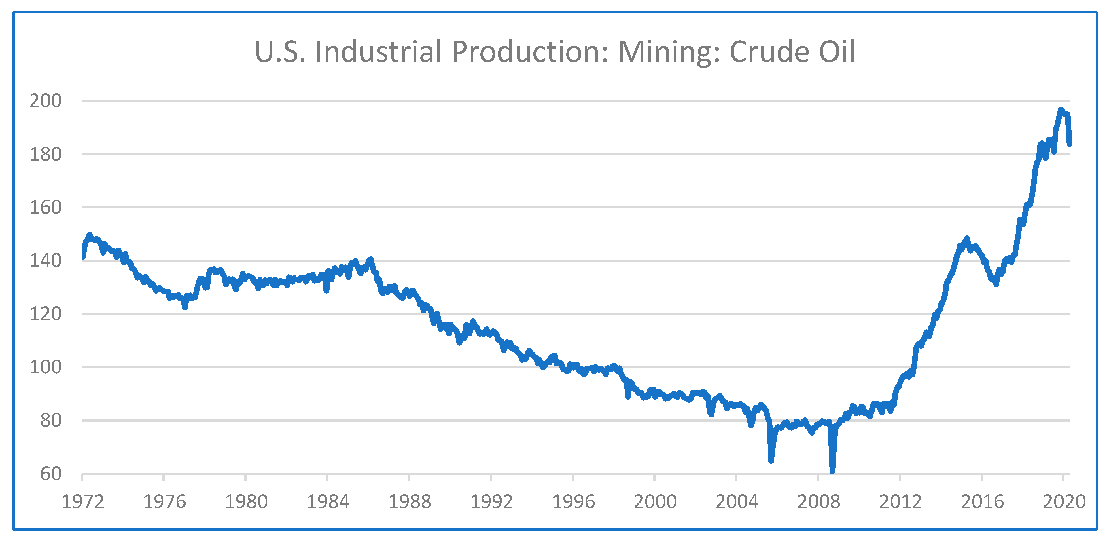
Figure 1 illustrates monthly crude oil production in the U.S. during the last 50 years. The shaded vertical columns represent U.S. recessions. From the early 1970s to the Great Financial Crisis of 2007–2009, U.S. oil production declined with a couple of exceptions; there was an increase during 1977–1979 and a period of production stability during 1979–1985. After the Global Financial Crisis, U.S. crude oil production increased rapidly with two periods of declines: the first occurred during May 2015 to October 2016 and the second from January 2020 to the end of this study in April 2020.

The U.S. was the world’s top oil producer from 1965 until the mid-1970s when Russia, (the former Union of Soviet Socialist Republics, USSR) replaced the U.S. In 1993, Saudi Arabia became the leading producer of oil and held this position until 2010. As Figure 1 illustrates, beginning at the end of the Global Financial Crisis in 2009, U.S. oil production began to increase, propelled by the shale technology, and by 2015, the U.S. regained the top position in the world as the largest oil producer.

The focus of this paper is to explain what factors contributed to the reversal of the declining trend in the U.S. crude oil production from 1970 to the Global Financial Crisis of 2007–2009. Daily news during the past decade of 2009–2019 reported that dramatic increases in U.S. crude oil production were the result of hydraulic fracturing, commonly described as fracking. The story has an additional component. The technology of hydraulic fracturing has been around for several decades and like most inventions it evolved over time. Modern day fracking did not begin until the 1990s. This happened when George P. Mitchell began using a new technique, which took hydraulic fracturing and combined it with horizontal drilling. Why did a modification of an existing technology suddenly become so widespread? Or, why did this shale oil production boom occur so long after the technology was created? We hypothesize that it was due to higher oil prices. The literature review emphasized the behavior of global crude oil prices during 2009–2019, remarking that this period was characterized by relatively high oil prices. Therefore, the fundamental hypothesis of this paper is that a few important economic variables played an essential role in the growth of U.S. oil production, and among them, the price of oil was the critical one. Data for the price of oil are obtained from the Federal Reserve Economic Data (FRED) at fred.stlouisfed.org. The global price of West Texas Intermediate (WTI) crude (POILWTIUSDM) is in U.S. dollars per barrel, not seasonally adjusted.

What other variables do we consider? First, global oil transactions are conducted in U.S. dollars and fluctuations in the value of the dollar versus other currencies affect oil quantities demanded, indirectly affecting U.S. oil production. We use the Trade Weighted U.S. Dollar Index: Broad, Goods and Services, (DTWEXBGS) not seasonally adjusted, available in FRED. Second, we propose that the price of copper is important because it is a proxy for global economic growth. FRED has data for the global price of copper (PCOPPUSDM) in U.S. dollars per metric ton, not seasonally adjusted. The third variable is the crude oil price volatility, calculated by the Chicago Board Options Exchange (CBOE) and called the Crude Oil Exchange Traded Fund (ETF) Volatility Index (OVXCLS), also available in FRED. The final variable we use is the Intercontinental Exchange Bank of America (ICE BofA) U.S. High Yield Index Option-Adjusted Spread (BAMLH0A0HYM2), expressed as a percent, not seasonally adjusted. These data represents the ICE BofA U.S. High Yield Index value, which tracks the performance of U.S. dollars denominated below investment grade rated corporate debt publicly issued in the U.S. domestic market. Such debt financed the majority of U.S. fracking investments in the discovery and extraction of oil. Major articles that discuss the role of these variables in detail include Malliaris and Malliaris (2018, 2020), Morana (2013), Narayan and Gupta (2015), Pinno and Serletis (2013), and Yin and Zhou (2016).

The dependent variable is the Industrial Production: Mining: Crude oil (IPG211111CN) Index (anchored in 2012 = 100), not seasonally adjusted. All data are monthly from July 2009 through April 2020 (130 rows). Initially, our data set started in June 2007 and ran to April 2020, but a break point analysis clearly indicated that there is a clear break into two subsets. The first subset spans from January 2007 to June 2009 that includes the Great Financial Crisis and the second spans from July 2009 to April 2020. Thus, we decided to focus on the second set. We used differences of logs as in (1), to ensure stationarity for all series. Detailed stationarity tests were performed that confirm our transformed data are stationary.

Symbolically, our model hypothesizes that:

Oil production, Y, is the dependent variable determined by price of oil X1, price of oil lagged one period X1(−1), price of copper X2, crude oil price volatility X3, price of trade weighted dollar X4, and high yield spread X5. Writing DLnXi, I = 1, 2, 3, 4, 5 means taking log differences for variable Xi. Symbolically we write

DLnY = f(DLnX1, DLnX1(−1), DLnX2, DLnX3, DLnX4, DLnX5)

(1)

We follow two distinct computational techniques to decide which inputs determine U.S. crude oil production. The first methodology is a standard econometric model and the second is a data mining model. We applied these to the same data set to address the question of factors affecting U.S. crude oil production. We found that the econometric approach, requiring model specification prior to inspecting the data set, is beneficial in identifying a structural break, but not in finding significant relationships among the variables. The data mining approach, which does not specify the form of the model a-priori, gives us more insight into the variable relationships and identifies a stronger relationship between actual and predicted values.

Variable Names:

Original Variable	Model Variable	Model Form
Oil Production	Y	DLnY
Price of Oil	X1	DLnX1
Lagged Price of Oil	X1(−1)	DLnX1(−1)
Price of Copper	X2	DLnX2
Volatility of Oil Price	X3	DLnX3
Trade Weighted Dollar	X4	DLnX4
High Yield Spread	X5	DLnX5

4. Econometric Methodology

The first step of the econometric methodology is testing for the stationarity of all variables. As indicated in the last section, the variables are non-stationary in levels using standard Augmented Dickey–Fuller and Phillips–Perron tests. Thus, we worked with first differences of the log variables. All the new transformed variables are stationary.

Second, we tested a linear version of our model in (1).

The results of

Table 1. Linear model: dependent variable: DLnY. Method: least squares. Sample (adjusted): 2007M06 to 2020M04. Included observations: 155 after adjustments.

Variable	Coefficient	Std. Error	t-Statistic	Prob.
C	0.005267	0.002336	2.255034	0.0256
DLnX1	0.055576	0.032028	1.735255	0.0848
DLnX2	−0.098202	0.048433	−2.027569	0.0444
DLnX3	0.018578	0.019516	0.951922	0.3427
DLnX4	0.095723	0.215945	0.443272	0.6582
DLnX5	0.008372	0.033034	0.253443	0.8003
R-squared	0.057970	Mean dependent variance		0.005506
F-statistic	1.833823	Durbin–Watson statistic		2.282259
Prob(F-statistic)	0.109590

show that the model is not strongly supported by the data. Economically meaningful variables, such as the price volatility of oil as an indicator of uncertainty, the weighted dollar as a determinant of currency fluctuations impacting the demand for oil, and the cost of financing oil exploration and extraction expressed by high yield rates of junk bonds; all these three independent variables are not significant in this linear model.

Repeated variations of this model, by also introducing lagged values and dropping insignificant variables, resulted in the following variation of the linear model presented in the Table below:

This model tells us that the actual current production of crude oil is influenced to a greater degree by the lagged price of oil, instead of the current price, perhaps because production cannot readily be adjusted. A second variable that impacts the crude oil production is the contemporaneous price of copper but with a negative sign. Our hypothesis that an increase in the price of copper signals industrial growth and that leads to more crude production is not supported by the data. So, we need to propose a new interpretation according to the evidence. Checking the data, we observe that the price of copper had a long downward trend from January 2011 to January 2017, reflecting some weakness in the global economy. This weakness was not strong enough to cause declines in the production of crude oil. The two opposite trends of declining copper prices and increasing oil production during the 6 years of the sample period, explain the negative sign for the copper coefficient. In particular, since 2016, the price of copper has been increasing, while oil prices have been decreasing, because the metal is needed in industrial digitalization.

In general, the results in

Table 2. Best model: dependent variable: DLnY. Method: least squares. Sample (adjusted): 2007M07 to 2020M04. Included observations: 154 after adjustments.

Variable	Coefficient	Std. Error	t-Statistic	Prob.
C	0.005566	0.002302	2.418038	0.0168
DLnX1(−1)	0.045873	0.023811	1.926517	0.0559
DLnX2	−0.109713	0.036894	−2.973740	0.0034
R-squared	0.062241	Mean dependent variance		0.005617
F-statistic	5.011095	Durbin–Watson statistic		2.281320
Prob(F-statistic)	0.007814

say that, if the price of oil last month increased, while the price of copper declined, oil producers continued to increase their crude oil production.

The third step was to determine our sample size by making sure the data used do not contain any breaks. Figure 1 illustrates that crude oil production was declining and after the Global Financial Crisis it reversed its trend and started increasing.

We indicated earlier that we tested a longer sample from early 1997 to the end of 2019 that indicated a break occurring in September/October 2008, exactly when the Lehman bankruptcy happened. We performed an additional test that allows for a break to be determined algorithmically.

Table 3. Sample breakpoint: dependent variable: DLnY. Method: least squares with breaks. Sample (adjusted): 2007M07 to 2020M04. Included observations: 154 after adjustments. Break type: Fixed number of globally determined breaks. Break: 2009M07. Allow heterogeneous error distributions across breaks.

Variable	Coefficient	Std. Error	t-Statistic	Prob.
2007M07-2009M06-24 obs
C	−0.000860	0.012657	−0.067938	0.9459
DLnX1(−1)	0.074640	0.103518	0.721034	0.4720
DLnX2	−0.174953	0.118824	−1.472370	0.1430
2009M07-2020M04-130 obs
C	0.006537	0.001435	4.554873	0.0000
DLnX1(-1)	0.041067	0.015763	2.605367	0.0101
DLnX2	−0.057188	0.030485	−1.875943	0.0626
R-squared	0.083305	Mean dependent variance		0.005617
F-statistic	2.689908	Durbin–Watson statistic		2.231942
Prob(F-statistic)	0.023359

shows the results of this search.

Based on the above analysis, we now propose a modified model (2) below. The results in

Table 4. Modified model: dependent variable: DLnY. Method: least squares. Sample: 2009M07 2020M04. Included observations: 130.

Variable	Coefficient	Std. Error	t-Statistic	Prob.
C	0.006537	0.001423	4.592360	0.0000
DLnX1(−1)	0.041067	0.015634	2.626810	0.0097
DLnX2	−0.057188	0.030236	−1.891383	0.0609
R-squared	0.066047	Mean dependent variance		0.006311
F-statistic	4.490564	Durbin–Watson statistic		2.061936
Log likelihood	353.0148
Prob(F-statistic)	0.013051

are the best our research has produced, and to gain further insight, we focus on the sample period 2009:07 to 2020:04 with 130 observations. This will avoid the parameter and/or volatility non-constancy issues. Consider the model below.

DLnY = c0 + c1 × DLnX1(−1) + c2 × DLnX2

(2)

The first result confirms that that DLnX1(−1) is relatively more important than DLnX1. This is also confirmed from the second methodology we present in the next section. The corresponding regression result also confirms this below. Table 4 also has a much better Durbin–Watson (DW) statistic. If it is close to two, then this implies that the residual is almost white noise. This is what is needed in modelling.

The result below is for the same sample and model without the constant.

In

Table 5. Model with no constant. Dependent variable: DLnY. Method: least squares. Sample: 2009M07 2020M04. Included observations: 130.

Variable	Coefficient	Std. Error	t-Statistic	Prob.
DLnX1(−1)	0.036782	0.016786	2.191198	0.0302
DLnX2	−0.055512	0.032520	−1.707014	0.0902
R-squared	−0.089046	Mean dependent varibale		0.006311
Log likelihood	343.0288
Durbin–Watson statistic	1.760206

, the DW statistic is not as good as the previous one. Additionally, the log likelihood value is less than that of the previous one. Thus, we prefer the model with a constant. To ensure high yield as an independent variable does not exhibit any significance, we also performed the additional test below:

DLn Y = c0 + c1 × DLnX1(−1) + c2 × DLnX2 + c3 × DLnX5

(3)

The sample is 2009:07–2020:04 and we checked whether the high yield spread variable had any impact. The result shows that it had virtually no impact. The results are displayed in

Table 6. Role of high yield spread. Method: least squares. Sample: 2009M07 2020M04. Included observations: 130.

Variable	Coefficient	Std. Error	t-Statistic	Prob.
C	0.006532	0.001429	4.571092	0.0000
DLnX1(−1)	0.040376	0.016283	2.479668	0.0145
DLnX2	−0.059846	0.034638	−1.727751	0.0865
DLnX5	−0.003372	0.021172	−0.159280	0.8737
R-squared	0.066235	Mean dependent variance		0.006311
Log likelihood	353.0279	Durbin–Watson statistic		2.063297
F-statistic	2.979192
Prob(F-statistic)	0.034035

below.

Finally, we questioned as to whether we could improve our discovered model. The results in Table 4 indicate parameter non-constancy (suggested by the break point). Although not reported, the Cumulative Sum of Squares (CUSUMSQ) test, using the residual of that model, suggests variance instability as well. In situations like this, it has been suggested in the literature that time varying variance in the time series may be incorporated. A relevant publication in this context is that by Rapach and Strauss (2008). It is, therefore, a good idea to allow generalized autoregressive conditional heteroskedasticity (GARCH) type residual variance and estimate the model without a breakpoint. This is the approach we adopted.

The GARCH model estimation used the conditional volatility specification as:

$$DLnY={\alpha }_0+{\alpha }_{1}DLnX1\left(-1\right)+{\alpha }_{2}DLnX2+{\epsilon }_t$$

$${\epsilon }_t~N\left(0,{\sigma }_t^2\right), {\sigma }_t^2={\beta }_0+{\beta }_1{\epsilon }_{t-1}^2+{\beta }_2{\sigma }_{t-1}^2$$

The estimation result is summarized in

Table 7. Dependent variable: DLnY. Method: ML ARCH—normal distribution (OPG—BHHH/Marquardt steps). Sample (adjusted): 2007M07 2020M04. Included observations: 154 after adjustments. Convergence not achieved after 500 iterations. Coefficient covariance computed using outer product of gradients. Presample variance: backcast (parameter = 0.7). GARCH = C(4) + C(5) × RESID(−1)^2 + C(6) × GARCH(−1).

Variable	Coefficient	Std. Error	z-Statistic	Prob.
C	0.007721	0.001737	4.444476	0.0000
DLnX1(−1)	0.048293	0.013430	3.595860	0.0003
DLnX2	−0.108885	0.032187	−3.382932	0.0007
Variance Equation
C	0.0000955	0.0000525	1.817618	0.0691
RESID(−1)^2	0.149577	0.031472	4.752722	0.0000
GARCH(−1)	0.599577	0.148010	4.050922	0.0001
R-squared	0.056773	Mean dependent variance		0.005617
Log likelihood	356.1520
Durbin–Watson statistic	2.269422

. It is evident that the parameters of the mean equation and the conditional variance equation are all highly significant. This indicates the suitability of the specification to address the concerns for parameter instability. This implies that it is probably the break point that caused the conditional variance to vary over time.

We also investigated the residual diagnostics from the model in Table 7. The most important ones for our case are the Q-statistic (indicates whether the residuals are uncorrelated) and Q-square statistic (indicates whether the squared residuals are uncorrelated). These two together should support the model specification. In this case, Q(12) = 9.025 and Q² (12) = 1.439. Both these support our model specification and indicate that both residuals and squared residuals have no autocorrelations up to lag 12.

The results reported in Table 7 corroborate the intuition offered in relation to Table 2, as far as the sign of the coefficients are concerned. In addition, the time varying variance captured by the GARCH specification makes the model specification robust.

5. Data Mining: Random Tree Modeling

The previous section reported several econometric tests and concluded that, for the period from July 2009 to April 2020, oil production was explained by two variables, the lagged price of oil and the price of copper. Surprisingly, the other four variables had little explanatory power. We then pursued a data mining methodology, which is significantly different from the econometric approach, to examine whether further insights can be found in this data set. We recognize that each approach has both advantages and shortcomings. For example, in the previous sections, we hypothesized an econometric model in the form of equations. In this section, in contrast, we allow the methodology to search the data set without an explicit functional relationship. We continue to use data from July 2009 to April 2020.

Using IBM’s SPSS Modeler 18.1 software, we ran a random tree model. This model is a collection of classification and regression tree models (C&RT). The C&RT model begins with all the input data in the root node and uses recursive partitioning to split these data into final groups where each group has similar target values.

From the root node, the algorithm makes a binary split, that is, it divides the data into two parts (called nodes) based on a value from one of the input variables to make the decision on how to divide the data. Each variable is considered as a possible splitting variable and the results are inspected by the model. The variable that is used at that point is the one that gives the most pure division of target values of the data. Thus, each resulting node will have more similar values of the target field and fewer dissimilar values. The same method is then applied to each of the nodes that resulted from the split. This process continues until stopping criteria are reached: a time limit, the number of splits that have occurred (tree depth), or no input variable allowing for a better division. In the ideal stopping place, each final node has very similar values of the target field.

The random tree model builds multiple C&RT models. For each model, the algorithm selects a random set of input rows from the training set (these are sampled with replacement). At each node as the tree is growing, the model selects a random set of inputs to inspect for possible splits (sampled with replacement). After running the specified number of trees, the model then runs all of the input data though every model and averages each row’s predicted values to obtain a final prediction for each row. In this case, we built 100 trees, each with a maximum depth of 10.

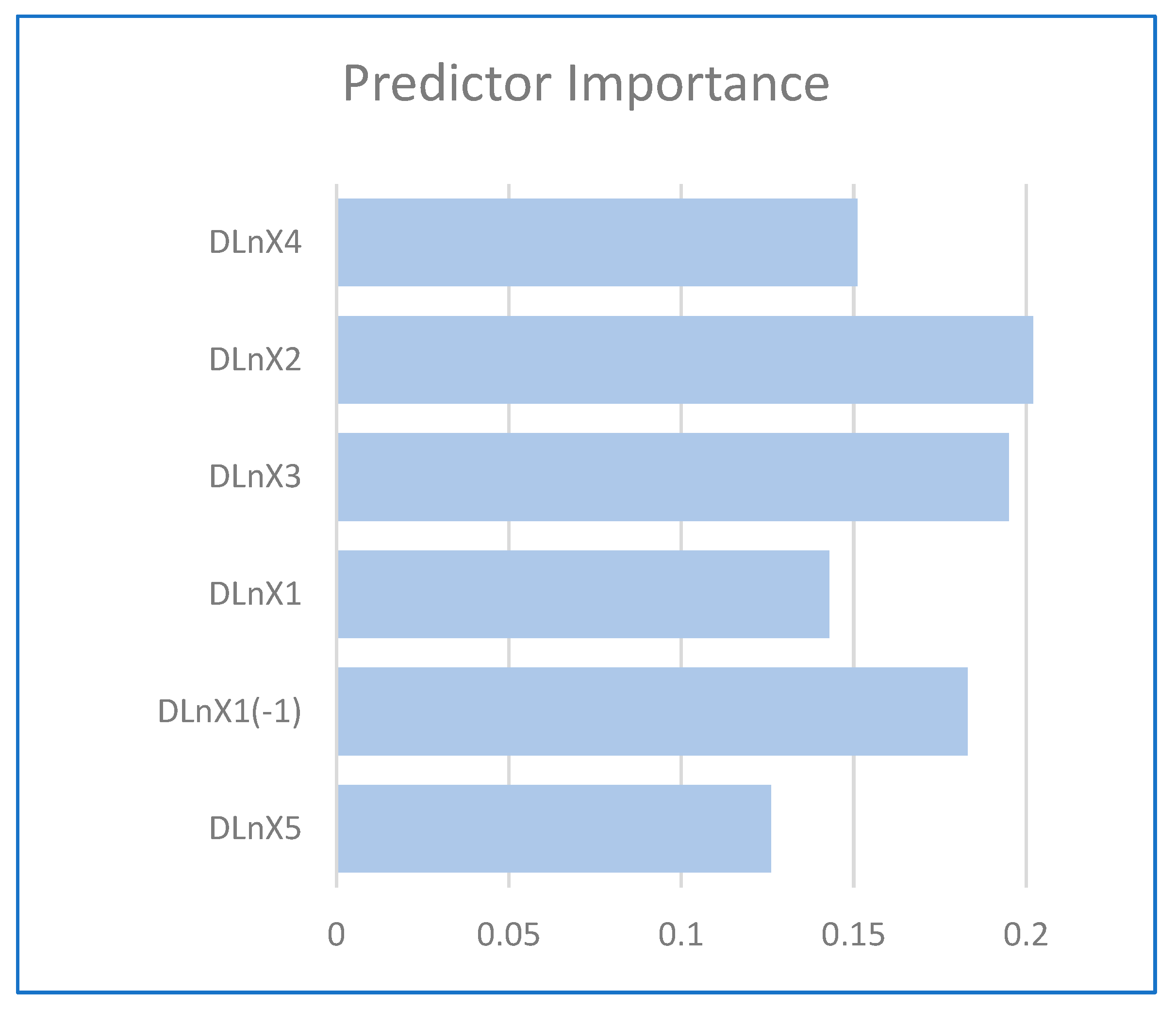
The accuracy of the model can be seen in the summary of the analysis node and in the graph of actual versus predicted values. Part of the modeler output includes the predictor importance chart. This shows the relative importance of each of the input variables to the model. The predictor importance values sum up to one. They do not indicate whether or not the model has done a good job in predicting the target value, rather they simply show how the generated model rated the importance of the inputs in making the predictions that it did. Predictor importance gives us an indication of which variables the model is most sensitive to. That is, a change in the value of the most important variables is more likely to cause a change in the value of the output.

Random Tree with One Lag for Oil

For this trial, we used data matching the period from the final econometric model, July 2009 through April 2020 (130 rows), with the five base variables and a 1-month lag of the oil price variable. The inputs, thus, included: DlnTWDollar (X4), DLnCopper (X2), DLnCrudeOilVolatility (X3), DLnOil (X1), Lagged DLnOil (X1(−1)), and DLnHighYieldSpread (X5). The target variable remained DLnProduction (Y).

The accuracy of the model is shown below with the statistics presented in

Table 8. Actual vs. predicted values of DLnProduction comparison.

Calculation for:	Value
Minimum Error	−0.036
Maximum Error	0.023
Mean Error	0.000
Mean Absolute Error	0.008
Standard Deviation	0.010
Linear Correlation	0.829
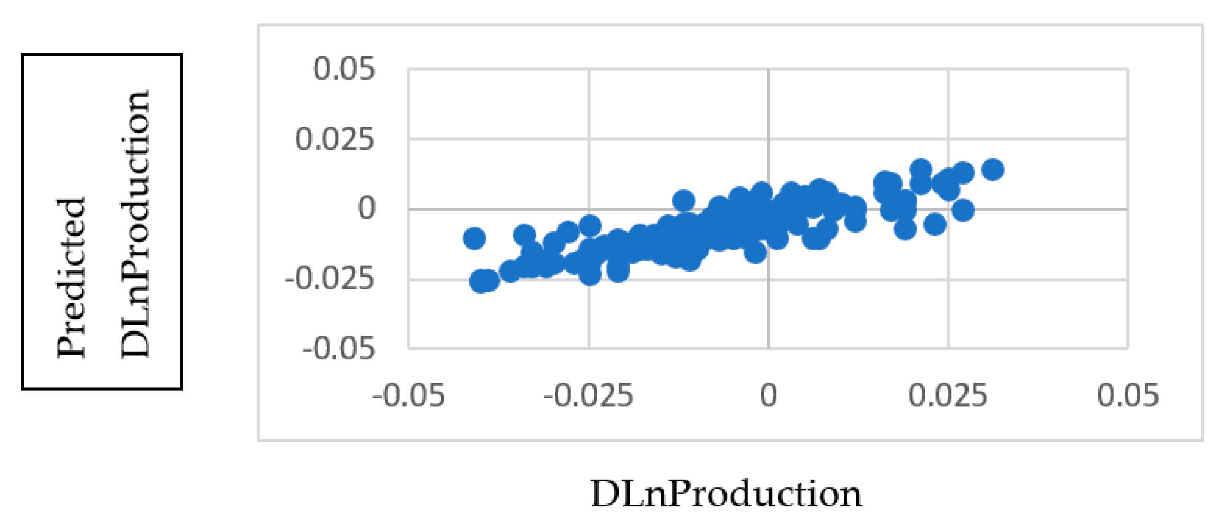
Occurences	130

, and a plot of the actual versus predicted target values. Notice that the linear correlation of the actual and predicted values is 0.829.

A plot of actual (DLnProduction) vs. predicted (USD R-DLnProduction) values of the target variable is shown in Figure 2. We see a linear grouping of predicted values with an outlier on the left.

The relative predictor importance, shown in Figure 3, shows that copper has the greatest relative importance, followed by crude oil volatility, and the lagged value of oil.

6. Conclusions

From the early 1970s to the Global Financial Crisis of 2007–09, U.S. crude oil production followed a declining trend. After the Global Financial Crisis, U.S. crude oil production increased rapidly. This paper addresses the important question: what factors have driven U.S. crude oil production since the Global Financial Crisis. We propose that factors such as: the price of oil, the one period lagged price of oil, the Trade Weighted U.S. Dollar Index, the price of copper, the crude oil price volatility and the high yield index spread, are important explanatory variables. Studies such as that by Malliaris and Malliaris (2020), found that the price of copper, the Trade Weighted Dollar Index and the U.S. high yield rate are statistically significant determinants for the price of oil. Pinno and Serletis (2013) and Yin and Zhou (2016) studied the influence of oil price volatility. Malliaris and Malliaris (2018), Morana (2013), and Narayan and Gupta (2015) found that the importance of these variables varies across regimes.

Using two modeling approaches—the random tree and multiple regression—we obtained the following results. The econometric methodology concludes that, relatively speaking, the one month lagged price of oil and the price of copper are the most significant explanatory variables for the upward trend of U.S. oil production. The data mining model ranks the six inputs in terms of importance. The top variable from this second methodology is the price of copper, followed by crude oil volatility, with the lagged price of oil coming in third. Combining both results, we conclude that the price of copper and the lagged price of oil emerge as significant explanatory variables in both approaches. This exercise also demonstrates the versatility of data mining techniques, the use of which is becoming increasingly popular in financial decision making. These data mining techniques are driven not by a model specification, but rather by data-driven relationships.