Know Your Clients’ Behaviours: A Cluster Analysis of Financial Transactions

Abstract

In Canada, financial advisors and dealers are required by provincial securities commissions and self-regulatory organizations—charged with direct regulation over investment dealers and mutual fund dealers—to respectively collect and maintain know your client (KYC) information, such as their age or risk tolerance, for investor accounts. With this information, investors, under their advisor’s guidance, make decisions on their investments that are presumed to be beneficial to their investment goals. Our unique dataset is provided by a financial investment dealer with over 50,000 accounts for over 23,000 clients covering the period from January 1st to August 12th 2019. We use a modified behavioral finance recency, frequency, monetary model for engineering features that quantify investor behaviours, and unsupervised machine learning clustering algorithms to find groups of investors that behave similarly. We show that the KYC information—such as gender, residence region, and marital status—does not explain client behaviours, whereas eight variables for trade and transaction frequency and volume are most informative. Hence, our results should encourage financial regulators and advisors to use more advanced metrics to better understand and predict investor behaviours.

1. Introduction

Investors hire financial advisors to help them select, facilitate, and manage their investment choices. In Canada, the client–advisor relationship varies by institution and regulatory regime. Some investors ask advisors to provide advice but ultimately make their own investment choices, other investors ask for a recommendation and then approve the advisor’s investment choices, while still others delegate full discretionary investment choices to the advisor. However, regardless of the relationship, advisors are expected and required by law to provide recommendations that are suitable for the client.

Suitability is described by regulators in Canada as a “meaningful dialogue with the client to obtain a solid understanding of the client’s investment needs and objectives, and to explain how a proposed investment strategy is suitable for the client in light of the client’s investment needs and objectives” (Ontario Securities Commission 2014). One of the suitability determinants for advisors is to determine the general investment needs and objectives of their client and any other factors necessary for them to determine whether a proposed purchase or sale is suitable (know your client or KYC). The assumption is that any subsequent purchases or sales (trading behavior) will conform to the KYC attributes and therefore be suitable.

In this paper, we consider unique interconnected datasets of financial transactions and KYC attributes to examine the relationship between KYC and trading behavior. The KYC data are comprised of objective demographic and identifying information and subjective financial situation information, where both are used to generate a client’s risk tolerance. We quantify trading behavior through metrics designed using an extended recency, frequency, and monetary (RFM) model from behavioral finance (Lumsden et al. 2008). We conduct our analysis using an unsupervised machine learning k-prototypes clustering algorithm (Huang 1997) and visualize the clusters using t-distributed stochastic neighbour embeddings (t-SNE) (van der Maaten and Hinton 2008). Our hypothesis is that groups of investors with similar KYC attributes will have the same risk tolerance and trading behaviours. KYC information should inform a risk tolerance score which the financial advisor—informed by suitability regulations—uses to delineate client investment transactions.

Using these advanced data analytics, our analysis shows that:

• Objective and subjective KYC data have little influence on trading behaviours.
• The distribution of risk tolerance across each clusters’ trading behavior is found to be similar, showing that trading behaviours may, on occasion, be inconsistent with the KYC-generated risk tolerance.
• KYC criteria appear to concentrate investors within narrow and rigid ‘swim lanes’ and appear to do a poor job of accommodating trading behaviours to the extremes—either highly risk-averse investors or those seeking higher risks.

At the onset, the hypothesis for this paper was that a thorough and complete assessment of investor KYC data should lead to an accurate determination of risk tolerance and suitability requirements. In turn, those determinations should manifest downstream in trading behavior and, eventually, in portfolio construction and investment outcomes (cf. Figure 1). In this paper, we focus on trading behavior, with investigations of portfolio construction, asset mix, and risk and returns left to future work.

Our conclusion that KYC data do not demonstrate a strong relationship to the trading behaviours exhibited by investors is important because “Know Your Client” is a foundational principle behind the concept of “suitability” and the corresponding investment regulatory framework deployed in many jurisdictions. See Ontario Securities Commission (2019) for a full discussion of the topic of KYC in Canada. The principle has also become more important as employers and governments de-risk retirement and savings programs post-2009 and move more of the burden of investment decision-making from professional portfolio managers to individual investors (Drolet and Morissette 2014). Furthermore, the topic has become more urgent given the events of early 2020.

Our algorithms clustered clients into one of five groups that were defined by their trading behavior, but all of which had similar suitability requirements. The clusters included:

• Cluster 1—active investors who trade frequently, in large amounts and appear sensitive to market influences,
• Cluster 2—younger savers who make regular, smaller deposits using automated platforms such as preauthorized chequing (PACs) and dollar cost averaging,
• Cluster 3—“just in time” savers who make infrequent trades at seemingly random intervals,
• Cluster 4—older investors who make regular withdrawals and cash out dividends and interest payments, and
• Cluster 5—systematic savers who make larger trades but make use of automation for predictable deposits and re-balancing.

Investor behavior is not only driven by the investor’s personal motives such as their goals and financial needs, but it is also influenced by the advisor relationship, dealer processes, regulatory obligations, and market influences (Cruciani 2017). As well, while the client onboarding and discovery process is foundational, it is also contextual and time-dependent, since the corresponding product recommendations are constantly changing in real-time. While the dataset and analysis used in this paper are unique, we are not privy to some of the subjective or undocumented influences and we cannot include them in our algorithms. It is therefore impossible for us to determine why the KYC process is not leading to the outcomes we would expect. Our analysis has inspired the question “Could protocols be improved?”, but we cannot answer the question without further research.

The paper reads as follows: Section 2 is a literature review on suitability and KYC regulations, trading behavior, and the use of machine learning algorithms in finance. Section 3 introduces the client and advisor financial data collected by the dealer, and develops the features that were used to measure client behaviours. Section 4 describes the machine learning methods used to identify investor groups based on their KYC information and behavior metrics. Section 5 shows the results from that clustering and Section 6 discusses the implications of the results and future work.

2. Literature Review

The literature review is broken down into three subsections of complementary areas in this work; investment suitability and KYC, trading behavior, and applications of machine learning in finance.

2.1. Investment Suitability and Know Your Client

Investors hire financial advisors who, in turn, recommend or distribute suitable financial products from investment dealers. The regulations for investment suitability for clients in Canada have been in place for decades and were formed through a collaboration of dealers, advisors, and regulators, with significant updates in 2009 (Ontario Securities Commission 2009). This paper studies the KYC obligation that requires financial advisors and dealers to conduct due diligence on clients and take “reasonable steps” to establish such things as their identity, creditworthiness, investment needs, financial objectives, and risk tolerance. The KYC obligation is designed to protect clients and advisors from unnecessary financial risk that does not align with the needs of the client, and ensure that advisors and dealers are acting in good faith.

Globally, most security regulators provide little guidance on how a firm or advisor should determine an investor’s risk profile. Instead, they rely on the judgment of the advisor or on processes created by the advisor’s firm to determine a consumer’s risk profile. These processes are typically embedded within the client onboarding and KYC protocols. As well, the KYC processes often include data attributes that extend beyond risk profiling to include basic client onboarding information or other regulatory requirements such as anti-money laundering (Simser 2020).

Several jurisdictions such as the UK, Europe and Australia do not prescribe an onboarding or KYC process but, instead, direct firms to “have a clear and robust process” (Brayman et al. 2015). In the US, Financial Industry Regulatory Authority (FINRA) rules require financial institutions to “use reasonable diligence, in regard to the opening and maintenance of every account, to know (and retain) the essential facts concerning every customer” (Financial Industry Regulatory Authority 2012) and that “a firm or associated person have a reasonable basis to believe a recommended transaction or investment strategy involving a security or securities is suitable for the customer” (Financial Industry Regulatory Authority 2020).

In Canada, we add a further level of complexity, since the investment industry is regulated by each province while, in some instances, securities regulation has been outsourced to national self-regulatory organizations (SROs). The dataset used in this paper falls under the purview of one of those SROs—the Investment Industry Regulatory Organization of Canada (IIROC) (Lokanan 2018). Aggregate IIROC members have a total of 10,002 advisors with, on average, $129,937,838 average assets under advisor (AUA) (Nash 2021), while the private dealer has 301 advisors with much less total investment per advisor with $15,005,190 AUA. The private dealer would rank in the top 20% of IIROC firms in terms of number of advisors and the firm’s clients are similar to their peers, except that the firm has very few clients from the province of Quebec.

To fulfill the KYC suitability requirement under IIROC regulations, advisors meet with clients to determine the client’s identity, investment needs, financial objectives and circumstances, and risk tolerance. Many, but not all, will use a formal questionnaire to help gather this information and score the risk tolerance. Questionnaires are not limited to these criteria, since regulators do not require a specific questionnaire, but require advisors to take “reasonable steps” to understand client needs.. An effective KYC protocol collects two types of information: (1) objective demographic information (legal identity), and (2) subjective information, from the perception of the client and their financial advisor, on the client’s investment needs, financial objectives, investment knowledge, appetite for risk and circumstances. For example, the questionnaire typically establishes the client’s identity by their full name, social insurance number, date of birth, address, and phone number. For investment needs, financial objectives and circumstances, they are asked about their income, net assets, living expenses, time horizon for the investment account, potential withdrawal of funds from the account over a year, how they would change their portfolio based on the market changes, how they set aside savings, plan for retirement, and make retirement savings plan contributions. To help determine risk tolerance, they are asked about investment knowledge, dependants, debt, willingness to take on risk-based on situational questions, and what they want to accomplish with their wealth. Research in the area of effective KYC protocols is at the emergent stage and has focused on the collection and evaluation of KYC information. The main focuses of research by the financial community have been on the objective information for improving compliance to prevent illegal or terrorist activities and decreasing the cost associated with increased compliance. Where KYC research exists, it tends to focus on cost efficiency-distributed ledger systems (Moyano and Ross 2017), how the financial crisis in the USA from 2007 to 2009 may have been affected due to non-compliance to US KYC regulations (Bilali 2011), on using KYC to protect client accounts (Mondal et al. 2016), and on improving auditor effectiveness in evaluating KYC compliance (De Smet and Mention 2011).

In contrast, few studies have been conducted to study the subjective information of the KYC obligation and their relationship to advisor and client investment behaviours, client investment objectives and outcomes, and dealer strategies to assist their advisors (Ontario Securities Commission 2015). Picard and de Palma (2010) reviewed a number of existing risk tolerance assessment tools and concluded that, while the neoclassical economic concept of risk tolerance is clear, its measurement through surveys is unclear. Since the economic definition of risk tolerance is a variation in future spending, many economists use questions that measure income volatility over time in order to assess risk tolerance. These questions are theoretically correct, but their performance as predictors of actual investment behavior during volatile stock markets is mediocre (Guillemette et al. 2012).

2.2. Trading Behavior

At the onset, the hypothesis for our research was that a thorough and complete assessment of an investor’s KYC data should lead to an accurate determination of their risk tolerance and suitability requirements. In turn, those determinations should manifest downstream in trading behavior and, eventually, in product recommendations, portfolio construction and investment outcomes.

In this paper, we look to better understand the relationship between collected KYC information and trading behaviors through applications of behavioral finance and statistical analysis. Behavioral finance is the intersection of psychology and finance to explain the trends and actions of financial markets, institutions, advisors, and individual investors. Behavioral finance has three main areas of application: analysis of patterns in stock returns, studying trading activity, and corporate finance (Subrahmanyam 2008). Our analysis focuses on trading activity. Our dataset encompasses over 23,000 clients who work with financial advisors at an anonymous investment dealer under the auspice of the IIROC regulatory regime. We use an extended RFM behavioral finance model (Lumsden et al. 2008) to engineer features for our machine learning algorithm. RFM models are used primarily in direct marketing to analyze customer behaviours through the recency of their last purchase, the frequency of their purchases, and how much is spent on each purchase. RFM models have been embedded in data mining algorithms (Birant 2011). To the best of our knowledge, RFM models have not been used in the context of trading activity of retail investors.

Several behavioral finance approaches to analyzing retail investors and financial advisors exist, where Zahera and Bansal (2018) provide a review of recent research that utilize data. One similar study of 46,969 Chinese retail investors was analyzed using cross-sectional regression and survival analysis and found that investors made decisions with specific behavioral biases, but they were inconclusive to whether those biases impacted each other (Chen et al. 2007). Another similar study of 665,533 Californian retail investors with non-discretionary financial advisors from January 1997 to June 1999 investigated abnormal trading volume and showed that retail investors are net buyers of attention-grabbing stocks (Barber and Odean 2008). Non-discretionary advisors require client approval for any trade or transaction on their account, while discretionary advisors need no such approval. Our research differs as we use unsupervised clustering to determine similarly behaving clients, and a modern Canadian dataset containing information on retail investors with discretionary and non-discretionary financial advisors.

Previous analyses on trading behaviours for Canadian investors with financial advisors have been conducted on transactional data of with demographic information for both clients and advisors. (Foerster et al. 2014) found that advisors influenced trading choices, but did not add enough value through recommendations to cover their fees in comparison to the performance of the unadvised. Their approach uses capital asset pricing modes, three-factor and four-factor models to study the excess returns for each advisor. Our approach differs, as we study account level trading behavior by creating features for a machine learning algorithm designed to determine the most important similarities of client trading behaviours.

Categories for investors or investor types have also been previously considered. These types can be distinguished by structural differences; usually domestic, international, or institutional investors, or some combination of all three (Che 2018; Grinblatt and Keloharju 2000). There also exist behavioral finance approaches to investor types that utilize personality theory (Pompian 2012), but these approaches tend to focus on personality traits associated with investing behavior (Kourtidis et al. 2017). In contrast, our research is a data-driven approach for relating client behaviours to KYC information to discover investor types.

2.3. Machine Learning Algorithms in Finance

Machine learning algorithms have been widely used in financial applications, such as risk modelling, return forecasting, and portfolio construction (Emerson et al. 2019), quantitative finance (Rundo et al. 2019), financial distress prediction (Huang and Yen 2019), banking risk management (Leo et al. 2019), credit-scoring models and financial crisis prediction (Lin et al. 2011), automation through artificial intelligence (Donepudi 2019), market prediction (Henrique et al. 2019), and credit risk modeling, detection of credit card fraud and money laundering, and surveillance of conduct breaches at financial institutions (Van Liebergen 2017). Popular algorithms used in these applications are support vector machines (Kim 2003), neural networks (West et al. 2005), and random forests (Patel et al. 2015).

Particularly in this paper, we are interested in clustering methods for financial trades and transactions. Recent work in this area includes agglomerative hierarchical clustering for asset allocation (Raffinot 2017) and aggregating stocks using dynamic time-series warping as a distance measure (Lim and Sin Ong 2020), self-organizing maps and k-means clustering methods in combination with classifier techniques to predict financial distress (Tsai 2014), fuzzy C-medoids clustering method for classifying financial time series (D’Urso et al. 2013), and clustering algorithms for financial risk analysis using multiple criteria decision-making methods (Kou et al. 2014). Absent from this body of work is the use of this broad class of techniques to analyze the suitability and client trading behaviours; the focus of this paper.

3. Data Description and Feature Engineering for Behavioral Finance

The data for this analysis are provided by a registered investment dealer that has provided investment products and technology to Canadian retail investors for over 30 years. The dealer hitherto has approximately 300 advisors who work with approximately 23,000 clients across Canada, with over $5 billion Canadian dollars (CAD) in assets. Clients typically have multiple accounts each with different purposes. For example, a client may have accounts for: (i) retirement savings; (ii) children’s education savings; and (iii) other savings. In total, clients with advisors who work with the dealer have over 50,000 accounts. The dealer provides a variety of financial products and services designed to support independent advisors. Furthermore, the dealer’s focus is to provide positive outcomes to clients and advisors, and not to push certain financial products.

In this section, we describe the KYC information and trades and transactions recorded in the data. We use descriptive analysis to demonstrate the demographics of our data and that the data is of good quality. We describe the features engineered from the data to be used in clustering, including unique metrics that measure client behaviours.

3.1. Data Description and Processing

The data are comprised of 52,025 accounts for 23,970 clients with associated KYC information, trade and transaction details from 1 January 2019 to 12 August 2019. The datasets were edited by the data donor prior to our receipt to ensure all client identifiers were anonymized consistent with Canada’s Personal Information Protection and Electronic Documents Act (PIPEDA) and standard research ethics protocols. Even using anonymization practices, there is still the possibility that clients could be identified using machine learning algorithms (Rocher et al. 2019). Therefore, no individuals will be identified or referenced in this paper and any subset of the data cannot be shared with readers.

The data are organized into linked datasets where entries were uniquely determined by an anonymized account ID or other relational database information. The specific datasets that we used are: (i) a KYC information dataset and (ii) a trades and transactions dataset. We created new features derived from both datasets that effectively supplement the KYC information with metrics that measure trading behaviours.

The data were processed by cleaning the data for improper entries (e.g., recording typos), transforming values into categories (e.g., grouping occupations into classifications), removing irrelevant, anonymized (e.g., contact information), or repeated (e.g., postal code in place of residence region) data. Any variable containing over 10 percent missing values or errors (e.g., ‘*’ or ‘unknown’) is removed to avoid excessive bias from imputation in our analysis. On the remaining data, imputation is conducted for each numeric and categorical feature based on existing values. For example, missing values in categorical variables such as ‘residency’ are filled with mode value ‘Ontario’ since more than 67% of clients are from Ontario; missing values in numerical variables such as ‘annual income’ are filled with mean income based on the job categories from KYC. See

Table A2. Summary of missing values and imputation for clustering.

Variable	Percent Missing	Action
Age	2.2%	Imputed with mean
Residency	0.47%	Imputed with mode
Risk tolerance	14.16%	Removed from clustering algorithm
Investment objective	6.7%	Removed clients with missing information
Annual income	0.13%	Imputed with mean
Investment knowledge level	7.8%	Removed clients with missing information
Gender	8.04%	Removed clients with missing information

in Appendix B for more details on missing data.

Table 1. Details of variables from clients’ KYC information.

Variable	Summary	Data Type	Example Values
Age	Ages range from 18 to 98 years old, with average at 57.4 years	Continuous	31 years old
Gender	$50.5\%$ male and $49.5\%$ female	Indicator	$M,F$
Residency	Province or Country or Region, with $70\%$ from Ontario	Categorical	ON, UK, USA, …
Annual income	Gross annual income in CAD	Continuous	Multiples of 100 between $1000 and $220,000 inclusive
Investment knowledge	The self-reported investment knowledge of poor (2%), fair (44%), good (37%), or sophisticated (17%)	Ordinal	1, 2, 3, or 4
Number of accounts	Clients can have more than one account	Ordinal	1,2,3,$\dots$10
Marital status	67% married, 18% single, 11% unknown and 4% divorced	Categorical	M, D, U, or S
Retirement indicator	The client’s retirement status	Indicator	Yes, No

shows the details of the pertinent objective KYC information. The distribution of client age is shown in Figure 2. The client age distribution is unimodal, centred at 58.1 years, has a standard deviation of 14.1 years, and is slightly left-skewed. The minimum age is 18 years—the legal age to open an account in Canada—and the maximum is 98.

The distribution of account residency is shown in

Table 2. Distribution of residency for client accounts. Locations are Ontario (ON), British Columbia (BC), Alberta (AB), Nova Scotia (NS), Canada (CA), United States of America (USA), United Kingdom (UK).

Location	ON	BC	AB	MB	NS	Other (CA)	Unknown	USA	UK
Percentage	65.19	14.63	12.00	3.94	2.59	0.92	0.41	0.26	0.06

, with the majority of accounts owned by clients in the province of Ontario. Figure 3 shows the distribution of annual income. The income distribution has an average of $$70,658$ and is right-skewed, with 50% of clients making less than $60 k. There are also income spikes at $50 k and $100 k, $150 k and $200 k.

Table 3. The number of clients by number of accounts.

Unique Accounts	1	2	3	4	5	6	7	8	9	10
Number of clients	5475	7659	6661	3051	775	222	79	40	4	4

shows the number of accounts per client. Approximately half of clients have two accounts or fewer, while 95% of clients have 4 accounts or less.

Our dataset contains a combination of trades and transactions for each client. We reserve the word “trades” for any interaction with mutual funds, stocks, securities, and bonds, and “transactions” for any interaction that does not include those interactions such as collecting dividends and interest. Trades are logged as orders, which are either active, inactive, filled, rejected, cancelled, or expired. In this paper, only filled orders are studied.

Each trade and transaction encompasses a number of data elements, including the type of product, transaction type, size, value, currency, security identification code, order date, process date, value date, and more. Using these trade and transaction datasets, we identified a spectrum of data elements that we believe could inform client behaviours, and then developed metrics using feature engineering to define and measure those client behaviours.

3.2. Feature Engineering

Feature engineering in data science is the process of using industry knowledge about data to construct metrics or “features” that can act as a measure for a quantity to be used in a machine learning model (Zheng and Casari 2018). Features generated from an RFM model can be used in conjunction with a machine learning algorithm (Anitha and Patil 2019). We construct features using objective and subjective KYC information, and trade and transaction information that we believe to be related to client investment behavior. Our features are an extension of an RFM model and fall into four categories: recency, frequency, monetary, and profile (RFMP).

The RFMP features are aggregated into a cross-sectional dataset that is static in time, where the cross-section is calculated on the last day recorded (12 August 2019) in the dataset.

Table 4. The recency, frequency, monetary profile (RFMP) features engineered from the dataset.

Feature Type	Description	Variables
Recency	Number of days since last trade on record	Days between the most recent trade date and 12 August 2019
Frequency	Total number of trades Average number of days between trades	Number of trades between first trade date and 12 August 2019 Number of days divided by number of trades since first trade day
Monetary	Buy and sell size totalsBuy and sell size minimum and maximum Trade size by type Variability of trade size by type	Third-party initiated trade type Dividends, income distribution, interest Systematic trade type Auto-withdrawal, pre-authorized contribution, asset allocation, reinvested dividend Periodic trade type Buys, sells, contribution, exchange, payment, electronic funds transfer (EFT), withdrawal, EFT deposit, tax-free savings account (TFSA) contribution, spousal contribution, redeems
Profile	KYC information Financial descriptors (e.g., number of accounts)	Age, gender, residency, annual income, investment knowledge level, number of accounts, marital status, retirement indicator

lists the features used for the clustering algorithm described in Section 4 and to generate the results shown in Section 5. We now describe each type.

Profile features describe the client as who they are and what their financial goals are. Commonly, they are considered influential factors to the behavior of the client (Foerster et al. 2017). Profile features are generated from KYC and account information for each of the clients. Some of the profile features were immediately ready for usage (for example, the time horizon of the account), whereas other variables needed to be derived; age in years is calculated from birth dates and the number of accounts is determined by searching the database for client accounts.

The recency feature is calculated as the number of days since a client’s most recent trade or transaction. The frequency features are calculated through a client’s overall trading pattern throughout the history of the dataset. These two feature types provide some information on their own, but when used together are more than the sum of their parts. For example, if a client has a large total number of trades (frequency) and months since their last trade (recency), this means they have a “burst” investing behavior. These feature types, when used together, provide an interesting picture of client behaviours.

The monetary features are engineered from trade and transaction amount details, rather than their temporal attributes. Specifically, a trade size multiplied by the value for each unit is the total monetary value in CAD, which we will refer to as the trade amount. If we looked at each trade as equivalent—similar to recency and frequency—then we will incorrectly consider that purchasing a stock is the same as re-investing a dividend. The stock purchase is an active trade that a client or advisor initiates, whereas a re-invested dividend is not. We classify trade sizes into the three metrics given by

$$\begin{array}{c}\hfill \begin{array}{cc}\hfill Third-partyinitiatedtradesize=& Dividend+Incomedistribution+Interest,\hfill \end{array}\end{array}$$

(1)

$$\begin{array}{c}\hfill \begin{array}{cc}\hfill Systematictradesize=& Autowithdrawal+Pre-authorizedcontribution+\hfill \\ \hfill & +Assetallocation+Reinvestdividend,\hfill \end{array}\end{array}$$

(2)

$$\begin{array}{c}\hfill \begin{array}{cc}\hfill Periodictradesize=& Buy\left(securities\right)+Sell\left(securities\right)+Contribution+Exchange\hfill \\ \hfill & +Payment+Electronicfundstransfer\left(EFT\right)+Withdrawal\hfill \\ \hfill & +EFTdeposit+TFSA+Spousalcontribution+Redeem,\hfill \end{array}\end{array}$$

(3)

where the descriptions of the trade types can be found in Appendix A. Third-party-initiated trades are comprised of trade types that are initiated by a third party, such as a coupon collected as cash from a bond. Systematic trades are comprised of self-imposed automatic investment strategies, such as an automatic monthly withdrawal from savings to purchase a mutual fund. Periodic trades are client- or advisor-initiated trades and transactions, such as an unscheduled purchase of a mutual fund for a TFSA.

Figure 4 shows the relative percentages of transaction sizes comprising the three behavioral metrics in Equations (1)–(3) versus time. For third-party-initiated trade size, dividend and income distribution dominate most of the transactions, and there appears to be a cyclical trend for dividends paid at the beginning of every month. For systematic trades, automatic withdrawal represents the majority of the feature size and has an obvious cyclical trend. There are spikes for asset allocation at the beginning of the year and six months in; a bi-annual cycle for asset allocations in systematic trades. For the periodic trades, the buy and sell types dominate without any cyclical trends.

The features that we engineer in this section are used directly as variables in our clustering model in Section 5. The next step is to take our engineered features and use them in a clustering algorithm. The theoretical underpinnings for our algorithm are described in the next section, which is followed by empirical results from clustering in the subsequent section.

4. Clustering Theory and Methods

Clustering is an unsupervised machine learning algorithm that is used to draw inferences about grouping commonalities from like-individuals in high dimensional data. It is a popular method for exploratory data analysis that finds previously unknown structures in data without specifying the underlying data generating process. Clustering is a powerful technique used in many fields, such as identifying fake news (Hosseinimotlagh and Papalexakis 2018), bioinformatics (Krishna and Murty 1999; Lan et al. 2018), text mining (Berry and Castellanos 2004), and wireless sensor networks (Abbasi and Younis 2007).

Clustering bears the task of grouping our set of clients by considering the similarity of their attributes and trading behavior (Xu and Wunsch 2008). For obvious reasons, we are interested in applications of clustering for financial data analytics (Le-Khac et al. 2012), particularly the area of behavior clustering analysis (BCA). Popular clustering algorithms used in this field are k-means (Steinley 2006) and k-modes (Chaturvedi et al. 2001; Huang and Ng 2003; Huang 1998). In this section, we introduce the k-prototypes algorithm that allows for both continuous and categorical data to cluster clients based on their similarity. Next, we introduce t-SNEs that reduce the dimensions of the data based on the similarity of each data point. The embeddings allow for data to be displayed in lower dimensions by similarity, while the clustering algorithm identifies the clusters among the data points.

4.1. k-Prototypes Clustering

The k-prototypes algorithm used here is similar to the k-means algorithm, where k-prototypes incorporate methods for including categorical data (Huang 1997). Suppose we have a set of N accounts, each with a unique identifier or index in the set $\mathcal{N}=\{1,2,\dots ,N\}$. The goal of any clustering algorithm is to put clients into k groups or clusters, such that

• each client is put into exactly one cluster;
• clients within a cluster have similar attributes; and
• clients in different clusters have dissimilar attributes.

The k clusters form a partition of the the client index set into k mutually exclusive subsets. Let ${\mathcal{N}}_{\ell }$ denote the set of client indices for all clients in cluster ℓ, $\ell =1,2,\dots ,k$, and ${\mathcal{P}}_{\mathcal{N}}=\{{\mathcal{N}}_1,{\mathcal{N}}_2,\dots ,{\mathcal{N}}_k\}$ denote the partition of the client index set. Furthermore, let $n_{\ell }$ denote the number of clients in cluster ℓ, such that ${\sum }_{\ell =1}^k{n}_{\ell }=N$.

Each client is described by their attribute vector $x_i,i=1,\dots ,N$, which is a combination of $p=15$ numeric variables (e.g., age) and $q=6$ categorical variables (e.g., marital status) and consists of one recency, two frequency, ten monetary, and eight profile variables. All attribute vectors contain the same variables. Without loss of generality, the numeric attributes occupy the first p positions of the attribute vector and the categorical attributes occupy the last q positions, giving

$$x_i=(\underset{\mathrm{numeric}}{\underbrace{x_{i1},x_{i2},\dots ,x_{ip}}},\underset{\mathrm{categorical}}{\underbrace{x_{i(p+1)},\dots ,x_{i(p+q)}}}).$$

(4)

The clustering algorithm works in an iterative fashion according to the following steps.

• Initialize the centroid (location) of the clusters by selecting k clients as “prototype” centroids.
• Allocate the clients to the clusters with the closest centroid.
• Compute an overall cost of the allocation by computing total distance of all clients from their assigned centroids.
• Update cluster centroids.
• Re-allocate the clients to the clusters with the closest (updated) centroid.
• Compute the overall cost by computing total distance.
• Iterate steps 4–6 until there is no change in the overall cost and output the clusters.

We kickoff the clustering party by randomly selecting k clients to serve as the initial centroids (locations) of the clusters. Specifically, the initial centroids are given by the attribute vectors of the randomly chosen k clients and are denoted by

$$c_{\ell }=(\underset{\mathrm{numeric}}{\underbrace{c_{\ell 1},c_{\ell 2},\dots ,c_{\ell p}}},\underset{\mathrm{categorical}}{\underbrace{c_{\ell (p+1)},\dots ,c_{\ell (p+q)}}}),\ell =1,\dots ,k,$$

(5)

where $c_{\ell j}$ is the cluster-ℓ, attribute-j centroid. Attributes in the centroid vectors are positioned in exactly the same order as in the client attribute vectors. As we shall see, as clusters are formed, the centroids get updated according to the individuals within each cluster.

After initializing the cluster centroids, we need some way of deciding how to put the clients into the clusters so that individuals within clusters are similar (close) and individuals across clusters are dissimilar (far apart). To measure the similarity between client i and cluster ℓ, we use the distance metric

$$\begin{array}{c}\hfill d(x_i,c_{\ell })=\sum _{n=1}^p\sqrt{{(x_{in}-c_{\ell n})}^2}+\sum _{n=p+1}^{p+q}\delta (x_{in},c_{\ell n}),\end{array}$$

(6)

where

$$\delta (a,b)=\left\{\begin{array}{cc}1\hfill & \mathrm{if}a\ne b\hfill \\ 0\hfill & \mathrm{for}a=b\hfill \end{array}\right..$$

(7)

Note that the distance metric is zero if, and only if, the attribute vector is exactly the same as the centroid, and if there are no categorical variables ($q=0$), then $d(·,·)$ is the usual Euclidean distance.

For client i, the distances between its attribute vector and each of the ℓ cluster centroids are computed, $d(x_i,c_{\ell }),\ell =1,\dots ,k$, and the client is placed in the closest cluster (e.g., minimum distance). This is done for all N clients (the clients initially chosen as centroids will clearly be placed in the correct cluster), with each client assigned to exactly one of the ℓ clusters.

After all clients are assigned to a cluster, the overall distance between individuals and their cluster centroid is computed by the cost function

$$\begin{array}{c}\hfill J=\sum _{\ell =1}^k\sum _{i\in {\mathcal{N}}_{\ell }}d(x_i,c_{\ell })\end{array}$$

(8)

The cluster centroids are updated by independently finding the middle for each cluster’s attributes. For the numeric attributes, the centroids are updated to be the within-cluster average value. Specifically, the updated j-th attribute for cluster ℓ is

$$\begin{array}{c}\hfill c_{\ell j}=\frac{1}{n_{\ell }}\sum _{i\in {\mathcal{N}}_{\ell }}{x}_{ij},j=1,\dots ,p.\end{array}$$

(9)

The categorical attributes of each cluster are updated using the mode given by

$$\begin{array}{c}\hfill c_{\ell j}=\mathbb{M}\left(x_{ij}|i\in {\mathcal{N}}_{\ell }\right)\end{array}$$

(10)

where $\mathbb{M}$ is the mode function. Next, we re-allocate each client to clusters using the minimum distance between the client attribute vector and the updated cluster centroids. After re-allocation, the overall cost is computed using Equation (8). If the total cost is unchanged from the previous iteration, we stop; otherwise, the cluster centroids are updated and clients are re-allocated. This is repeated until the total cost function is unchanged.

Since the initial set of k cluster centroids (e.g., k clients serving as initial centroids) is chosen randomly, the clustering process is repeated for a large number of randomly chosen initial cluster centroids to better search for the global minima of the cost function. Each initial cluster centroid produces clusters and their total cost. The best (and final) cluster is the one that minimizes the cost function over all randomly chosen initial cluster centroids. Typically, it is infeasible to look at all possible k initial cluster centroids, which is the reason for the random sampling of the initial cluster centroids. For example, with N = 25,000 clients and $k=5$ clusters, the number of possible ways of choosing the initial cluster centroids is $\frac{25,000\times 24,999\times 24,998\times 24,997\times 24,996}{5!}$ which is an infeasible number of possibilities to examine.

4.2. Visualizing Clusters—t-Distributed Stochastic Neighbor Embeddings

Visualizing high-dimensional data by projecting it onto a lower-dimensional space is commonly used (Yang 1999). The computationally efficient dimensionality reduction tool used herein is the t-distributed stochastic neighbour embeddings (t-SNE) (van der Maaten and Hinton 2008). The t-SNE method provides a significant dimensionality reduction from high dimensional data to two or three dimensions while preserving the significant structure. This method is a nonlinear mapping which, as opposed to linear mappings such as principal components analysis, performs better for preserving the local structure of data. That is, this method keeps similar clients close together in a low-dimensional visualization. This is important for visualizing clusters since we use a clustering method that evaluates clients by their similarity. Therefore, the t-SNE method creates a map of clients based on their similarity, and then we independently apply the clustering algorithm to the data—all without specifying the data generating process.

For the t-SNE method, “perplexity” is an important parameter that affects the visual behavior of data projection. Different datasets require different perplexities to display the clustering—or lack thereof—features present in the data. According to van der Maaten and Hinton (2008), the perplexity can be viewed as the algorithm’s method to measure the number of effective nearest neighbours, with typical values between 5 and 50. Choosing the perplexity value requires the user to tune it during the modelling process. There is no standard method for specifying the perplexity value. Furthermore, larger datasets require a larger perplexity (van der Maaten 2009). For our dataset, the perplexity value is set to 200 to obtain a stable embedded data plot.

5. Results

In this section, we discuss the results of applying the method described in Section 4 to the client data discussed in Section 3. The data cleaning, feature engineering, clustering algorithm, t-SNE visualization, and analysis are implemented using Python version 3.6 and R version 3.5.3 (R Core Team 2020). The implementation of the k-prototypes clustering algorithm originated from a GitHub repository (de Vos 2020) and the t-SNE algorithm used for data visualization is in the sklearn Python package (Pedregosa et al. 2011). The next step is to use the k-prototypes clustering algorithm to identify the optimal number of clusters for this client dataset.

5.1. Choosing the Optimal Number of Clusters

Two clustering performance evaluation methods are used to determine the optimal number of clusters: the silhouette coefficient and the Davies–Bouldin (DB) score. The silhouette coefficient (Rousseeuw 1987) compares the cluster membership classification of each client by comparing their similarity within and between clusters and indicates how well clients are assigned. The Silhouette coefficient of client i in cluster ${\mathcal{N}}_{\ell }$ is defined as

$$\begin{array}{c}\hfill S_i=\frac{b_i-a_i}{max(a_i,b_i)},\end{array}$$

(11)

where $a_i$ is a similarity measure of client i to clients within their cluster given by

$$\begin{array}{c}\hfill a_i=\frac{1}{|{\mathcal{N}}_{\ell }|-1}\sum _{j\in {\mathcal{N}}_{\ell },j\ne i}d(x_i,x_j),\end{array}$$

and $b_i$ is a similarity measure of client i to the clients in the most similar or closest neighbouring cluster given by

$$\begin{array}{c}\hfill b_i=\underset{g\in \{1,2,...,k\},g\ne \ell }{min}\left[\frac{1}{|{\mathcal{N}}_g|}\sum _{j\in {\mathcal{N}}_g}d(x_i,x_j)\right].\end{array}$$

The best assignment value for the silhouette coefficient is 1 and the worst value is $-1$. Values near 0 indicate overlapping clusters. Negative values generally indicate that a client may be poorly assigned, as a different cluster is more similar. The top panel of Figure 5 shows the average Silhouette coefficient $S=\frac{1}{N}{\sum }_{i=1}^N{S}_i$ for $k=2$ to 8 clusters. The average silhouette coefficient is maximized for this clustering method when we choose $k=5$ clusters.

The DB score (Davies and Bouldin 1979) is another cluster partition evaluation metric that compares the similarity between clusters with the size of the clusters themselves. The DB score is calculated as

$$\begin{array}{c}\hfill DB=\frac{1}{k}\sum _{i=1}^k\underset{j\ne i}{max}\left(\frac{e_i+e_j}{d(c_i,c_j)}\right)\end{array}$$

(12)

where k is the number of clusters, $e_i$ is the average distance of all clients in cluster i from the centroid $c_i$, namely $e_i=\frac{1}{{\mathcal{N}}_i}{\sum }_{j\in {\mathcal{N}}_i}d(x_j,c_i)$. The DB index quantifies the density of clusters, with the index decreasing as separation between the clusters increases. Similar to the averaged silhouette coefficient, the bottom panel in Figure 5 indicates that $k=5$ cluster is optimal.

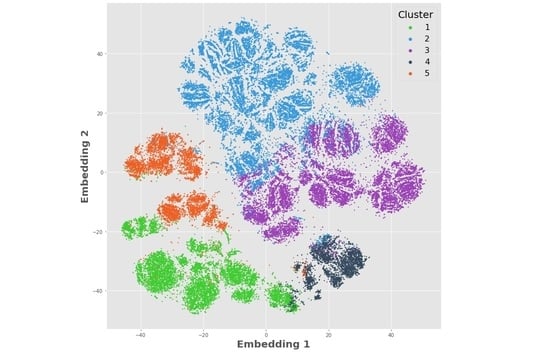
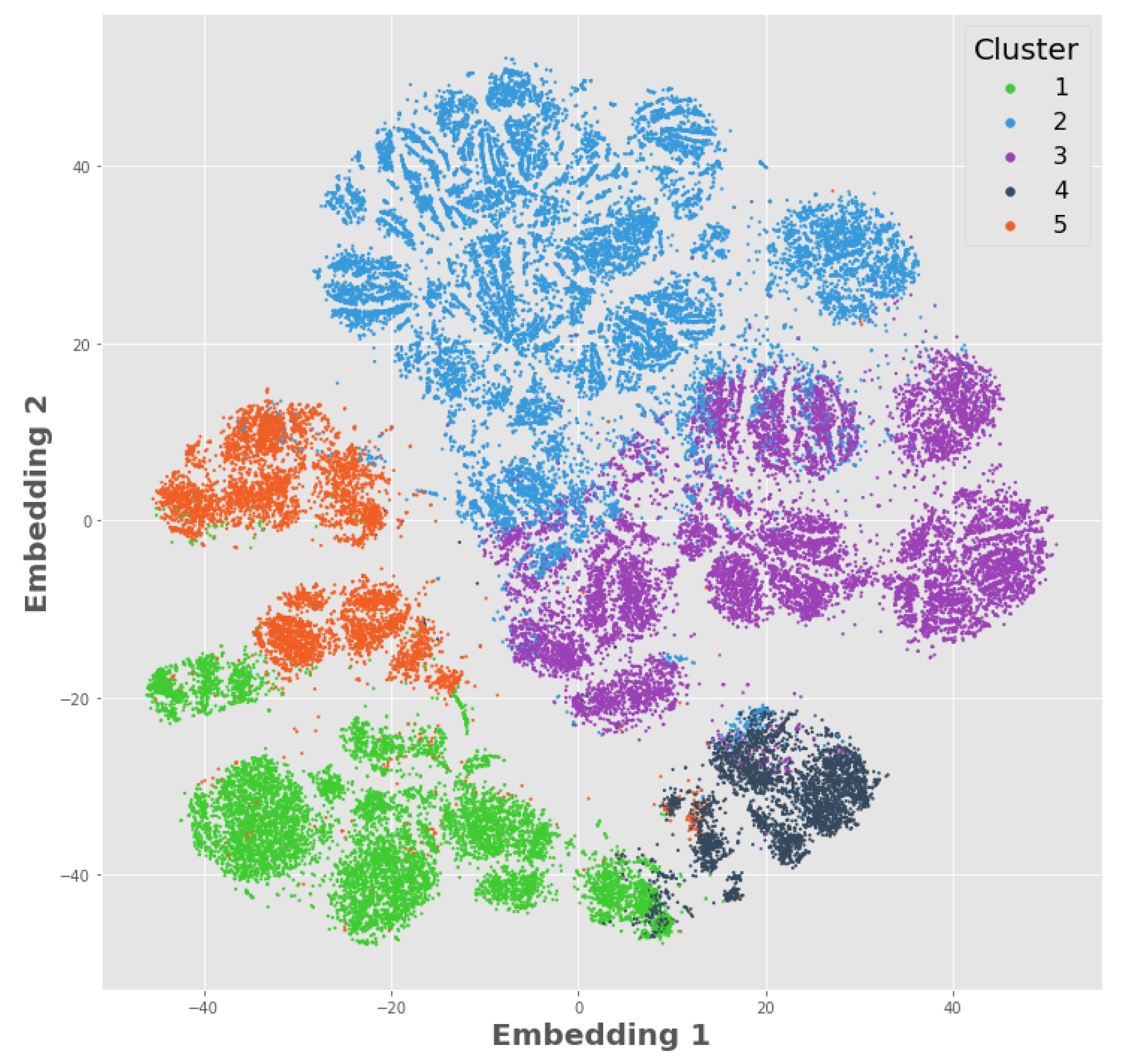
5.2. Cluster Visualization Using t-SNE

Figure 6 shows the overlaid cluster membership on the t-SNE visualization with a perplexity of 200. Among the 5 clusters, cluster 1 has 19% of the clients and its data points are green on the embedding map, cluster 2 has the largest portion of clients with (36%) and is labelled blue, cluster 3 has 27% of clients and is labelled purple, cluster 4 the least portion (7%) of clients and labelled black, and cluster 5 has 12% of clients and is labelled orange.

From the two-dimensional embedding map in Figure 6, there are distinct boundaries between clusters 2, 3 and clusters 1, 4, 5. There are overlaps between clusters 1 and 5, clusters 2 and 3, and clusters 1 and 4. It is noteworthy that higher dimensional embedding can reveal other higher-order boundaries that distinguish these overlapped clusters. The projection from three dimensions to these two dimensions creates the visual appearance of overlapping.

5.3. Within Cluster Analysis

Table 5. Mean values of the numeric features of the optimal cluster centroids. The column colours assigned to each cluster are universal in this paper.

Cluster	1	2	3	4	5
Age (years)	58.7	55.5	59.6	64.5	57.9
Annual gross income (CAD)	72,310.11	72,623.69	69,397.60	62,229.89	69,955.47
Investment knowledge level	2.69	2.70	2.68	2.84	2.70
Number of accounts	3.07	3.03	3.05	2.85	2.89
Recency (days)	57.9	179.59	179.9	153.8	61.9
Frequency (trades per day)	5.77	0.006	0.0004	0.46	1.32
Days between trades	5.15	179.46	179.9	151.93	85.18
Mean third-party trade (CAD)	98.01	17.19	102.21	63.40	109.07
SD third-party trade (CAD)	79.13	7.51	57.69	46.17	57.23
Mean systematic trade (CAD)	350.08	22.34	292.90	946.09	251.61
SD Systematic trade (CAD)	25.53	0.13	0.11	671.11	0.35
Mean periodic trade (CAD)	36,064.08	72.09	22,071.42	11,543.26	14,060.87
SD periodic trade (CAD)	27,685.31	0.71	12,190.73	16,335.76	12,828.52

summarizes the mean values of the numeric features for each cluster. These mean values are the numeric attributes of the centroids (location) of the optimal clusters. Figure 6 and Table 5 demonstrate the following patterns between each of the clusters:

• Clusters 1 (green) and 5 (orange) are similar in their demographics and trade types, but cluster 5 trades less often with smaller periodic trade sizes.
• Cluster 2 (blue) is distinct from the others where they are largely inactive in their trading.
• Clusters 3 (purple) and 4 (gray) are similar, except that cluster 3 makes larger, less frequent trades and cluster 4 utilizes larger systematic trades.

Figure 7 shows the clustering results for categorical features. For the residency and gender features, there are no obvious differences between clusters. For the age feature, cluster 4 has a high average age, and the distribution is left-skewed and appears almost bimodal. Clusters 1, 3 and 5 have similar age distributions. The cluster 2 age distribution appears shifted left and has younger clients compared to other clusters. The bottom right panel shows the percentages of the six account types in different clusters. Clients in clusters 1, 3 and 5 have similar account proportions. Cluster 2 has more cash accounts and cluster 4 has more RIF accounts.

Figure 8 shows the monthly average trade amount over time, where the shaded areas are 95% bootstrapped pointwise confidence intervals. Top, middle, and bottom panels correspond to third party initiated trades, systematic trades, and periodic trades, respectively. We note first the scale of each type of trade in the figure, where there are three different orders of magnitude across the three panels. This is caused by the nature of the trade types or by the number of elementary trade types within each of the classes defined in Equations (1)–(3).

• For third-party-initiated trades, cluster 4 has a relatively high trade amount and the largest volatility. Cluster 1 has similarly high trade amounts, but less volatility. Clusters 3 and 5 have very similar trade amounts and volatilities that are smaller than the trade amounts and volatilities of clusters 1 and 4. Cluster 2 has the lowest average trade size and volatility.
• For systematic trades, a similar pattern to third-party-initiated trades is reflected. Clusters 1 and 4 are again similar in the trade amount and volatility, with cluster 4 having slightly larger amounts except in June. Clusters 3 and 5 have almost identical average trade amounts except in August, and cluster 2 has the smallest average trade amount. An interesting aspect of all clusters is the peaks for the average trade amount evident in January and June.
• Cluster 1 dominates the periodic trade amounts, while cluster 2 has almost zero periodic trade amounts on average, with very little volatility. Clusters 3 to 5 have similar trade amounts and volatilities, except in February and March when there is a slight peak before trending down for clusters 3 and 5. Clusters 3 to 5 all have an uptick in the average trade amount in July.

Figure 9 shows the KYC-inferred risk tolerance (RT) score distribution of clients for each cluster. The majority of clients in each cluster’s distribution (top four and bottom left panels) have a RT score close to three. Furthermore, each distribution appears to be quite similar, with smaller upticks at RT scores of two and four. The panel in the bottom right shows the overlaid densities of each cluster, where the reddish-brown area is the shape that all clusters share.

We investigated the similarity of these distributions using a parametric ANOVA comparison of client RT score means and a nonparametric Kruskal–Wallis test comparison of means (Kruskal and Wallis 1952; McKight and Najab 2010), for which both tests’ null hypotheses were rejected with p-values $\le 2\times {10}^{-16}$ and $3.23\times {10}^{-79}$, respectively. A post hoc analysis of a comparison of individual groups with adjusted P-values for multiple comparisons was conducted using Tukey’s test (Tukey 1949) for ANOVA and the nonparametric Dunn’s test (Dunn 1964) for Kruskal–Wallis test. The results of these tests are shown in Appendix C. These results suggest that clusters 3 and 4 have significantly different distributions from the rest. We investigated the difference in distributions using the histogram density estimators (Figure 9) in a pairwise symmetric Kullback–Liebler (KL) plug-in estimator (Kullback and Leibler 1951; Ramírez et al. 2004; Wang et al. 2005). The KL estimator shows that the difference between the unlike-clusters’ divergences (3, 4) is not much larger than the like-clusters (1, 2, 5) divergences. The results of the symmetric KL estimators are shown in Appendix C.

From the analysis of the distributions KYC-inferred RT scores, we conclude that the distributions are similar, even though there exists a statistically significant difference between the distributions (not practically different). A smaller sample of points from each distribution would have a difficult time rejecting the null hypotheses of an analysis of variance test. The mean pattern and shape of risk tolerance distributions do not line up with what we expected. Clusters 1 and 4 are the most striking. Cluster 4 is demographically skewed towards older investors and we would expect to see RT scores weighted towards scores 1.0, 2.0 or 3.0. There are, in fact, only 15.7% of clients in cluster 4 who have less than a 3.0 RT score. Behaviourally, cluster 1 appears to pursue a riskier trading strategy and we would, therefore, have expected to see a strong weighting towards observations in the 4.0 to 5.0 RT score range. In fact, 14.8% of cluster 1 clients fall into the 4.0 to 5.0 RT score range.

5.4. From Data to People—Personas

The cluster memberships are determined by the similarity of individuals, and we are interested in studying how the groups differ from each other. Using the plots and information presented heretofore, we summarize how the clusters differ using the most important variables to their cluster classification. We note that individuals from two different groups may appear similar, but they are classified based on subtle differences determined by the clustering algorithm.

Using our understanding of investors and finance, we have created ‘personas’ for clients to ease discussions and help understand the groups as real people and not just data. The five personas are as follows:

• Cluster 1: Active Traders (19% of investors) trade frequently (weekly and monthly) and in large amounts. The pattern of trades is seemingly random and initiated manually. These investors had investments across a spectrum of accounts (mainly registered savings plans (RSPs) and TFSAs), and were of an “average” age distribution and demographic. They had a derived risk tolerance rating that averaged 3.19 with standard deviation 0.63, where 1 is a low or preservative risk tolerance and 5 is high or aggressive.
• Cluster 2: Early Savers (36%) never actively trade and instead rely on systematic transactions (auto-withdrawal, pre-authorized contribution, asset allocations). This group tended to have investments in cash accounts and to be younger. They had a derived risk tolerance rating that averaged 3.18 with standard deviation 0.75.
• Cluster 3: Just-In-Time (27%) initiate trades manually but far less frequently than Cluster 1 and in smaller amounts. These investors had investments across a spectrum of accounts (RSPs, TFSAs, etc.), and were of an “average” age and demographic. They had a derived risk tolerance rating that averaged 3.12 with standard deviation 0.73.
• Cluster 4: Older Investors (7%) trade infrequently and the trades were either initiated systematically or from a third-party (pre-authorized withdrawals, dividends and other disbursements). This cluster had an above average concentration of RIFs, and tended to be older. They had a derived risk tolerance rating that averaged 2.95 with standard deviation 0.71.
• Cluster 5: Systematic Savers (12%) trade recurrently (every 60, 90, or 120 days), in small amounts driven by systematic processes (dollar cost averaging) and periodic trading. These investors had investments across a spectrum of accounts (RSPs, TFSAs etc.), and of an “average” age and demographics. They had a derived risk tolerance rating that averaged 3.19 with standard deviation 0.76.

Table 6. KYC demographics and trading behaviours compared to expected risk tolerance and anticipated risk tolerance for each cluster. Risk tolerances are calculated on a scale of 1 to 5, where 1 is a low or preservation risk tolerance and 5 is high or aggressive.

			Clusters
Client Trait	1—Active Traders	2—Early Savers	3—Just-in-Time	4—Older Investors	5—Systematic Savers
KYC	Average age, income and demographics. Average investment knowledge. Average $ accounts and balances	Slightly younger but average income and demographics. Average investment knowledge. Average $ accounts and balances	Average age, income and demographics. Average investment knowledge. Average $ accounts and balances	Older but average, income and demographics. Average investment knowledge. Average $ accounts and balances	Average age, income and demographics. Average investment knowledge. Average $ accounts and balances
Trade behavior	Trade frequently in large amounts and appear sensitive to market influences	Smaller, regular deposits making use of PACs	Infrequent trades at seemingly random intervals	Primarily withdrawals, dividends, and interest payments	Larger, systematic trades and re-balancing
Risk tolerance observed average	3.19/5	3.18/5	3.12/5	2.95/5	3.19/5
Risk tolerance anticipated	5/5	4/5	3/5	1/5	2/5

provides a high-level description of the clusters and the trading behavior that defined them. In general, the clusters were defined by how often they traded, how much they traded and the mechanisms they used to affect their trades. For example, cluster 1 (active traders) traded frequently, in relatively larger amounts and in asymmetrical amounts. In contrast, cluster 5 (systematic savers) also traded in relatively larger amounts, but used automated mechanisms to trade on a prescribed time frame (for example monthly) and in the same amount each time (dollar cost averaging). However, regardless of their trading behavior, all five clusters had virtually identical risk tolerances (on a scale of 1 to 5) which were derived by the advisor and the firm from the investors’ KYC information. As a result, there appears to be a disconnect between the assumption that an investor’s objectives will be expressed through their trading behavior and governed by their risk tolerance and suitability constraints (KYC).

6. Discussion and Future Plans

We have conducted a variety of approaches to analyze the client dataset to extract financial behaviours. We have constructed data summaries and extracted features that we believe capture financial behaviours, and included those summaries and features in a descriptive analysis. The features engineered from our data will directly affect the performance of future predictive models we are developing. We conducted a k-prototypes clustering algorithm on extracted features, where the cluster memberships were determined by minimizing a similarity cost function. We evaluated our clustering method using a silhouette coefficient and a DB score, and found that 5 clusters was optimal. We analyzed the clustering results using the centroids generated by the algorithm and t-SNE visualizations. Each cluster features demonstrated unique personas: clients in cluster 1 were frequent traders, clients in cluster 2 were largely inactive in trading, clients in cluster 3 made large, infrequent and aperiodic trades, clients in cluster 4 were older investors who primarily made withdrawals, and clients in cluster 5 were large systematic traders. We found that there was not a practical difference between the KYC-determined risk score distributions of the clusters.

Our analysis is unique in comparison to previous studies. Firstly, our data set is more current than similar studies (Foerster et al. 2014). Secondly, our data encompass financial advice, a critical dimension of investor decision making and behavior when the majority of investors rely on professional advisors for their investment decisions. Our analysis also includes an extensive array of financial instruments (stocks, mutual funds, ETFs, and so forth), where previous studies have tended to focus on subsets of the investment opportunities available to retail investors (Barber and Odean 2013; Foerster et al. 2014). Lastly, to the best of our knowledge, this is the first paper that clusters investors on both their investment behavior and KYC information.

Our findings tend to challenge some of the widely held assumptions in the financial advice industry regarding risk tolerance and trading behavior. For example, the assumption that risk tolerance is, or should be, driven by age (Charles and Kasilingam 2013; Talpsepp 2013), gender (Arano et al. 2010; Barber and Odean 2001; Hsu et al. 2020), or income (Anderson 2013; Isidore and Christie 2019). We found that none of these factors played a significant role in our clustering. Instead, the clusters were driven by trading behavior and we assume that those trading behaviours are driven in turn by investor preferences. Presumably, advisors should be able to use these insights to better manage investor preferences and achieve investment outcomes that are more strongly aligned with the investor’s objectives.

Given the lack of a defined standard for KYC processes, the conclusions reached in this paper should not be extended with confidence beyond our dataset and the IIROC regime. However, we believe our analytical methodologies can be applied to other datasets, in other jurisdictions, and the authors would welcome the opportunity to collaborate with other scholars on that basis.

The ultimate goal of our research program, of which this paper is the first step, is to provide enhanced advice to clients and their advisors using both traditional and digital approaches. The projects described herein are a path to attain that goal, providing the necessary algorithms to give information and advice in good faith. The projects not only support digitally assisted advice, but the results can be used to report to regulatory committees on how data-driven results can aid regulators in promoting financial wellness policies.

Moving forward, we will examine the behaviours of the clusters against the suitability and KYC protocols noted in this paper and then attempt to determine if those behaviours have a constructive or destructive impact on client outcomes. We also plan to examine the impact that advisor behaviours have on the analysis noted above, while looking for evidence for whether we can change or nudge any or all of the noted behaviours. Previous research has determined that traditional characteristics explain only 12 percent of an investor’s portfolio allocations (Foerster et al. 2014, 2017), (Grace 2014; Linnainmaa et al. 2018). Our goal is to use new, sophisticated technologies to help examine the remaining 88 percent of unexplained investor behavior (Grace 2019). We will investigate the trade and asset mix of this dataset to examine whether the trading behavior identified in each cluster is “suitable”—as defined by the prescribed regulations—by studying security risk ratings—as defined by industry. We also plan to examine portfolio returns to estimate the probability of a successful outcome relative to the investment goals of each client, and to look for evidence to see if the advisor’s behavior is influencing trading behavior consistent with the KYC and suitability requirements.

References

1. Abbasi, Ameer Ahmed, and Mohamed Younis. 2007. A survey on clustering algorithms for wireless sensor networks. Computer Communications 30: 2826–41. [Google Scholar] [CrossRef]
2. Anderson, Anders. 2013. Trading and under-diversification. Review of Finance 17: 1699–741. [Google Scholar] [CrossRef]
3. Anitha, Palaksha, and Malini M. Patil. 2019. RFM model for customer purchase behavior using k-means algorithm. Journal of King Saud University-Computer and Information Sciences. [Google Scholar] [CrossRef]
4. Arano, Kathleen, Carl Parker, and Rory Terry. 2010. Gender-based risk aversion and retirement asset allocation. Economic Inquiry 48: 147–55. [Google Scholar] [CrossRef]
5. Barber, Brad M., and Terrance Odean. 2001. Boys will be boys: Gender, overconfidence, and common stock investment. The Quarterly Journal of Economics 116: 261–92. [Google Scholar] [CrossRef]
6. Barber, Brad M., and Terrance Odean. 2008. All that glitters: The effect of attention and news on the buying behavior of individual and institutional investors. The Review of Financial Studies 21: 785–818. [Google Scholar] [CrossRef] [Green Version]
7. Barber, Brad M., and Terrance Odean. 2013. The behavior of individual investors. In Handbook of the Economics of Finance. Amsterdam: Elsevier, vol. 2, pp. 1533–70. [Google Scholar]
8. Berry, Michael W., and Malu Castellanos. 2004. Survey of text mining. Computing Reviews 45: 548. [Google Scholar]
9. Bilali, Genci. 2011. Know your customer—Or not. University of Toledo Law Review 43: 319. [Google Scholar]
10. Birant, Derya. 2011. Data mining using RFM analysis. In Knowledge-Oriented Applications in Data Mining. London: IntechOpen. [Google Scholar]
11. Brayman, Shawn, Michael Finke, Ellen Bessner, J. E. Grable, Paul Griffin, and Rebecca Clement. 2015. Current practices for risk profiling in Canada and review of global best practices. In Study Prepared for the Investor Advisory Panel of the Ontario Securities Commission. Available online: https://www.osc.gov.on.ca/documents/en/Investors/iap_20151112_risk-profiling-report.pdf (accessed on 20 January 2021).
12. Charles, A., and Ramaiah Kasilingam. 2013. Does the investor’s age influence their investment behaviour? Paradigm 17: 11–24. [Google Scholar] [CrossRef]
13. Chaturvedi, Anil, Paul E. Green, and J. Douglas Caroll. 2001. k-modes clustering. Journal of Classification 18: 35–55. [Google Scholar] [CrossRef]
14. Che, Limei. 2018. Investor types and stock return volatility. Journal of Empirical Finance 47: 139–61. [Google Scholar] [CrossRef]
15. Chen, Gongmeng, Kenneth A. Kim, John R. Nofsinger, and Oliver M. Rui. 2007. Trading performance, disposition effect, overconfidence, representativeness bias, and experience of emerging market investors. Journal of Behavioral Decision Making 20: 425–51. [Google Scholar] [CrossRef]
16. Cruciani, Caterina. 2017. Investor Decision-Making and the Role of the Financial Advisor: A Behavioural Finance Approach. Cham: Springer. [Google Scholar]
17. Davies, David L., and Donald W. Bouldin. 1979. A cluster separation measure. IEEE Transactions on Pattern Analysis and Machine Intelligence, 224–27. [Google Scholar] [CrossRef]
18. de Vos, Nico. 2020. Python Implementations of the k-Modes and k-Prototypes Clustering Algorithms, for Clustering Categorical Data. Available online: https://github.com/nicodv/kmodes (accessed on 20 January 2021).
19. Donepudi, Praveen Kumar. 2019. Automation and machine learning in transforming the financial industry. Asian Business Review 9: 129–38. [Google Scholar] [CrossRef]
20. Drolet, Marie, and René Morissette. 2014. New facts on pension coverage in Canada. Insights on Canadian society. Statistics Canada Catalogue. [Google Scholar]
21. Dunn, Olive Jean. 1964. Multiple comparisons using rank sums. Technometrics 6: 241–52. [Google Scholar] [CrossRef]
22. D’Urso, Pierpaolo, Carmela Cappelli, Dario Di Lallo, and Riccardo Massari. 2013. Clustering of financial time series. Physica A: Statistical Mechanics and Its Applications 392: 2114–29. [Google Scholar] [CrossRef]
23. Emerson, Sophie, Ruairí Kennedy, Luke O’Shea, and John O’Brien. 2019. Trends and applications of machine learning in quantitative finance. Paper presented at 8th International Conference on Economics and Finance Research (ICEFR 2019), Lyon, France, June 18–21. [Google Scholar]
24. Financial Industry Regulatory Authority. 2012. Rule 2090. Know Your Client. Available online: https://www.finra.org/rules-guidance/rulebooks/finra-rules/2090 (accessed on 20 January 2021).
25. Financial Industry Regulatory Authority. 2020. Rule 2111. Suitability. Available online: https://www.finra.org/rules-guidance/rulebooks/finra-rules/2111 (accessed on 20 January 2021).
26. Foerster, Stephen, Juhani T. Linnainmaa, Brian T. Melzer, and Alessandro Previtero. 2014. The Costs and Benefits of Financial Advice. Working Paper. Available online: https://www.hbs.edu/faculty/Shared%20Documents/conferences/2013-household-behavior-risky-asset-mkts/Costs-and-Benefits-of-Financial-Advice_Foerster-Linnainmaa-Melzer-Previtero.pdf (accessed on 20 January 2021).
27. Foerster, Stephen, Juhani T. Linnainmaa, Brian T. Melzer, and Alessandro Previtero. 2017. Retail financial advice: Does one size fit all? The Journal of Finance 72: 1441–82. [Google Scholar] [CrossRef]
28. Grace, Chuck. 2014. Practitioner’s Summary: The Costs and Benefits of Financial Advice. Available online: https://restless.co.uk/course/practitioners-guide-to-cost-benefit-analysis-udemy-133053/ (accessed on 20 January 2021).
29. Grace, Chuck. 2019. Next-Gen Financial Advice: Digital Innovation and Canada’s Policymakers. Toronto: CD Howe Institute Commentary 538. [Google Scholar]
30. Grinblatt, Mark, and Matti Keloharju. 2000. The investment behavior and performance of various investor types: A study of finland’s unique data set. Journal of Financial Economics 55: 43–67. [Google Scholar] [CrossRef]
31. Guillemette, Michael, Michael S. Finke, and John Gilliam. 2012. Risk tolerance questions to best determine client portfolio allocation preferences. Journal of Financial Planning 25: 36–44. [Google Scholar]
32. Henrique, Bruno Miranda, Vinicius Amorim Sobreiro, and Herbert Kimura. 2019. Literature review: Machine learning techniques applied to financial market prediction. Expert Systems with Applications 124: 226–51. [Google Scholar] [CrossRef]
33. Hosseinimotlagh, Seyedmehdi, and Evangelos E. Papalexakis. 2018. Unsupervised content-based identification of fake news articles with tensor decomposition ensembles. Paper presented at Workshop on Misinformation and Misbehavior Mining on the Web (MIS2), Los Angeles, CA, USA, February 9. [Google Scholar]
34. Hsu, Yuan-Lin, Hung-Ling Chen, Po-Kai Huang, and Wan-Yu Lin. 2020. Does financial literacy mitigate gender differences in investment behavioral bias? Finance Research Letters, 101789. [Google Scholar] [CrossRef]
35. Huang, Yu-Pei, and Meng-Feng Yen. 2019. A new perspective of performance comparison among machine learning algorithms for financial distress prediction. Applied Soft Computing 83: 105663. [Google Scholar] [CrossRef]
36. Huang, Zhexue, and Michael K. Ng. 2003. A note on k-modes clustering. Journal of Classification 20: 257. [Google Scholar] [CrossRef]
37. Huang, Zhexue. 1997. Clustering large data sets with mixed numeric and categorical values. In Proceedings of the First Pacific Asia Knowledge Discovery and Data Mining Conference. Singapore: World Scientific, pp. 21–34. [Google Scholar]
38. Huang, Zhexue. 1998. Extensions to the k-means algorithm for clustering large data sets with categorical values. Data Mining and Knowledge Discovery 2: 283–304. [Google Scholar] [CrossRef]
39. Isidore, Renu, and P. Christie. 2019. The relationship between the income and behavioural biases. Journal of Economics, Finance, and Administrative Science 24: 127–44. [Google Scholar] [CrossRef]
40. Kim, Kyoung-jae. 2003. Financial time series forecasting using support vector machines. Neurocomputing 55: 307–19. [Google Scholar] [CrossRef]
41. Kou, Gang, Yi Peng, and Guoxun Wang. 2014. Evaluation of clustering algorithms for financial risk analysis using MCDM methods. Information Sciences 275: 1–12. [Google Scholar] [CrossRef]
42. Kourtidis, Dimitrios, Prodromos Chatzoglou, and Zeljko Sevic. 2017. The role of personality traits in investors trading behaviour: Empirical evidence from greek. International Journal of Social Economics 44: 1402–20. [Google Scholar] [CrossRef]
43. Krishna, K., and M. Narasimha Murty. 1999. Genetic k-means algorithm. IEEE Transactions on Systems, Man, and Cybernetics, Part B (Cybernetics) 29: 433–39. [Google Scholar] [CrossRef] [Green Version]
44. Kruskal, William H., and W. Allen Wallis. 1952. Use of ranks in one-criterion variance analysis. Journal of the American Statistical Association 47: 583–621. [Google Scholar] [CrossRef]
45. Kullback, Solomon, and Richard A. Leibler. 1951. On information and sufficiency. The Annals of Mathematical Statistics 22: 79–86. [Google Scholar] [CrossRef]
46. Lan, Kun, Dan-tong Wang, Simon Fong, Lian-sheng Liu, Kelvin K. L. Wong, and Nilanjan Dey. 2018. A survey of data mining and deep learning in bioinformatics. Journal of Medical Systems 42: 139. [Google Scholar] [CrossRef] [PubMed]
47. Le-Khac, Nhien-An, Cai Fan, and Tahar Kechadi. 2012. Clustering approaches for financial data analysis. Paper presented at 8th International Conference on Data Mining, Las Vegas, NA, USA, July 16–19. [Google Scholar]
48. Leo, Martin, Suneel Sharma, and Koilakuntla Maddulety. 2019. Machine learning in banking risk management: A literature review. Risks 7: 29. [Google Scholar] [CrossRef] [Green Version]
49. Lim, Tristan, and Chin Sin Ong. 2020. Portfolio diversification using shape-based clustering. The Journal of Financial Data Science. [Google Scholar] [CrossRef]
50. Lin, Wei-Yang, Ya-Han Hu, and Chih-Fong Tsai. 2011. Machine learning in financial crisis prediction: A survey. IEEE Transactions on Systems, Man, and Cybernetics, Part C (Applications and Reviews) 42: 421–36. [Google Scholar]
51. Linnainmaa, Juhani T., Brian T. Melzer, and Alessandro Previtero. 2018. The Misguided Beliefs of Financial Advisors. Kelley School of Business Research Paper (18-9). Available online: https://ssrn.com/abstract=3101426 (accessed on 25 January 2021).
52. Lokanan, Mark E. 2018. Securities regulation: Opportunities exist for IIROC to regulate responsively. Administration & Society 50: 402–28. [Google Scholar]
53. Lumsden, Shelly-Ann, Srikanth Beldona, and Alastair M. Morrison. 2008. Customer value in an all-inclusive travel vacation club: An application of the RFM framework. Journal of Hospitality & Leisure Marketing 16: 270–85. [Google Scholar]
54. van der Maaten, Laurens, and Geoffrey Hinton. 2008. Visualizing data using t-sne. Journal of Machine Learning Research 9: 2579–605. [Google Scholar]
55. McKight, Patrick E., and Julius Najab. 2010. Kruskal-wallis test. In The Corsini Encyclopedia Of Psychology. Hoboken: John Wiley & Sons. [Google Scholar]
56. Mondal, Prakash Chandra, Rupam Deb, and Mohammad Nurul Huda. 2016. Transaction authorization from know your customer (KYC) information in online banking. Paper presented at 2016 9th International Conference on Electrical and Computer Engineering (ICECE), Dhaka, Bangladesh, December 20–22; pp. 523–26. [Google Scholar]
57. Moyano, José Parra, and Omri Ross. 2017. KYC optimization using distributed ledger technology. Business & Information Systems Engineering 59: 411–23. [Google Scholar]
58. Ontario Securities Commission, Investor Advisory Panel. 2015. Current Practices for Risk Profiling in Canada and Review of Global Best Practices. Toronto: Ontario Securities Commission. [Google Scholar]
59. Nash, Maria. 2021. Investment Industry Association of Canada, Toronto, ON, Canada. Personal Communication, January 11. [Google Scholar]
60. Ontario Securities Commission. 2009. National Instruments 31-103. Available online: https://www.osc.gov.on.ca/en/SecuritiesLaw_31-103.htm (accessed on 20 January 2021).
61. Ontario Securities Commission. 2014. CSA Staff Notice 31-336—Guidance for Portfolio Managers, Exempt Market Dealers and Other Registrants on the Know-Your-Client, Know-Your-Product and Suitablility Obligations. Available online: https://www.osc.gov.on.ca/documents/en/Securities-Category3/csa_20140109_31-336_kyc-kyp-suitability-obligations.pdf (accessed on 20 January 2021).
62. Ontario Securities Commission. 2019. Amendments to National Instrument 31-103 Registration Requirements, Exemptions and Ongoing Registrant. Available online: https://www.osc.gov.on.ca/en/SecuritiesLaw_ni_20191212_31-103_amendments-ongoing-registrant-obligations.htm (accessed on 20 January 2021).
63. Patel, Jigar, Sahil Shah, Priyank Thakkar, and Ketan Kotecha. 2015. Predicting stock and stock price index movement using trend deterministic data preparation and machine learning techniques. Expert Systems with Applications 42: 259–68. [Google Scholar] [CrossRef]
64. Pedregosa, Fabian, Gael Varoquaux, Alexandre Gramfort, Vincent Michel, Bertrand Thirion, Olivier Grisel, Mathieu Blondel, Peter Prettenhofer, Ron Weiss, Vincent Dubourg, and et al. 2011. Scikit-learn: Machine learning in Python. Journal of Machine Learning Research 12: 2825–30. [Google Scholar]
65. Picard, Nathalie, and André de Palma. 2010. Evaluation of MiFID Questionnaires in France. Technical Report. Paris: AMF. [Google Scholar]
66. Pompian, Michael M. 2012. Behavioral Finance and Investor Types: Managing Behavior to Make Better Investment Decisions. Hoboken: John Wiley & Sons. [Google Scholar]
67. R Core Team. 2020. R: A Language and Environment for Statistical Computing. Vienna: R Foundation for Statistical Computing. [Google Scholar]
68. Raffinot, Thomas. 2017. Hierarchical clustering-based asset allocation. The Journal of Portfolio Management 44: 89–99. [Google Scholar] [CrossRef]
69. Ramírez, Javier, Jaume C. Segura, Carmen Benítez, Angel De La Torre, and Antonio J. Rubio. 2004. A new kullback-leibler vad for speech recognition in noise. IEEE Signal Processing Letters 11: 266–69. [Google Scholar] [CrossRef]
70. Rocher, Luc, Julien M. Hendrickx, and Yves-Alexandre De Montjoye. 2019. Estimating the success of re-identifications in incomplete datasets using generative models. Nature Communications 10: 1–9. [Google Scholar] [CrossRef] [PubMed]
71. Rousseeuw, Peter J. 1987. Silhouettes: A graphical aid to the interpretation and validation of cluster analysis. Journal of Computational and Applied Mathematics 20: 53–65. [Google Scholar] [CrossRef] [Green Version]
72. Rundo, Francesco, Francesca Trenta, Agatino Luigi di Stallo, and Sebastiano Battiato. 2019. Machine learning for quantitative finance applications: A survey. Applied Sciences 9: 5574. [Google Scholar] [CrossRef] [Green Version]
73. Simser, Jeffrey R. 2020. Canada’s financial intelligence unit: FINTRAC. Journal of Money Laundering Control 23: 297–307. [Google Scholar] [CrossRef]
74. De Smet, Dieter, and Anne-Laure Mention. 2011. Improving auditor effectiveness in assessing KYC/AML practices: Case study in a luxembourgish context. Managerial Auditing Journal 26: 182–203. [Google Scholar] [CrossRef]
75. Steinley, Douglas. 2006. k-means clustering: A half-century synthesis. British Journal of Mathematical and Statistical Psychology 59: 1–34. [Google Scholar] [CrossRef] [Green Version]
76. Subrahmanyam, Avanidhar. 2008. Behavioural finance: A review and synthesis. European Financial Management 14: 12–29. [Google Scholar] [CrossRef]
77. Talpsepp, Tõnn. 2013. Does gender and age affect investor performance and the disposition effect? Research in Economics and Business: Central and Eastern Europe 2. [Google Scholar]
78. Tsai, Chih-Fong. 2014. Combining cluster analysis with classifier ensembles to predict financial distress. Information Fusion 16: 46–58. [Google Scholar] [CrossRef]
79. Tukey, John W. 1949. Comparing individual means in the analysis of variance. Biometrics 5: 99–114. [Google Scholar] [CrossRef]
80. van der Maaten, Laurens. 2009. Learning a parametric embedding by preserving local structure. Paper presented at Twelfth International Conference on Artificial Intelligence and Statistics, Clearwater Beach, FL, USA, April 16–18; Volume 5 of Proceedings of Machine Learning Research. Edited by D. van Dyk and M. Welling. pp. 384–91. [Google Scholar]
81. Van Liebergen, Bart. 2017. Machine learning: A revolution in risk management and compliance? Journal of Financial Transformation 45: 60–67. [Google Scholar]
82. Wang, Qing, Sanjeev R. Kulkarni, and Sergio Verdú. 2005. Divergence estimation of continuous distributions based on data-dependent partitions. IEEE Transactions on Information Theory 51: 3064–74. [Google Scholar] [CrossRef]
83. West, David, Scott Dellana, and Jingxia Qian. 2005. Neural network ensemble strategies for financial decision applications. Computers & Operations Research 32: 2543–59. [Google Scholar]
84. Xu, Rui, and Don Wunsch. 2008. Clustering. Hoboken: John Wiley & Sons, vol. 10. [Google Scholar]
85. Yang, Li. 1999. 3D grand tour for multidimensional data and clusters. In Advances in Intelligent Data Analysis. Edited by D. J. Hand, J. N. Kok and M. R. Berthold. Berlin and Heidelberg: Springer, pp. 173–84. [Google Scholar]
86. Zahera, Syed Aliya, and Rohit Bansal. 2018. Do investors exhibit behavioral biases in investment decision making? A systematic review. Qualitative Research in Financial Markets 10: 210–51. [Google Scholar] [CrossRef]
87. Zheng, Alice, and Amanda Casari. 2018. Feature Engineering for Machine Learning: Principles and Techniques for Data Scientists, 1st ed. Newton: O’Reilly Media, Inc. [Google Scholar]
Figure 1. The downstream footprints of know your client (KYC) regulations.
Jrfm 14 00050 g001
Figure 2. Distribution of client ages, where each bin contains one year.
Jrfm 14 00050 g002
Figure 3. Distribution of client annual incomes. The vertical dotted lines represent the three quartiles at $40 k, $60 k, and $100 k.
Jrfm 14 00050 g003
Figure 4. The relative percentage of transactions sizes from the three behavioral metrics versus time (January to August 2019). Top, middle, and bottom panels correspond to third-party-initiated, systematic, and periodic trades, respectively.
Jrfm 14 00050 g004
Figure 5. The top panel shows the average Silhouette coefficient and the bottom panel shows the DB score for versus number of clusters. The optimal number of clusters is identified by the red circle at the elbow.
Jrfm 14 00050 g005
Figure 6. t-SNE visualization for the full dataset by cluster projected onto two embeddings.
Jrfm 14 00050 g006
Figure 7. Categorical and numerical distributions of clusters. (Top left) panel shows the residency distribution, (top right) shows the gender distribution, (bottom left) shows the age distribution, and (bottom right) shows the account type distribution for each cluster.
Jrfm 14 00050 g007
Figure 8. Cluster average trading amounts with 95% bootstrapped confidence intervals versus time. (Top), (middle), and (bottom) panels correspond to third-party-initiated trades, systematic trades, and periodic trades, respectively.
Jrfm 14 00050 g008
Figure 9. KYC-Inferred RT score distributions by cluster. The top four and bottom left panels are each cluster’s distribution by inferred RT scores. The bottom right panel is an overlay of the clusters’ RT score distributions.
Jrfm 14 00050 g009