Article

Simultaneous Analysis of Insurance Participation and Acreage Response from Subsidized Crop Insurance for Cotton

Department of Agricultural and Resource Economics, The University of Arizona, Tucson, AZ 85721, USA
*
Author to whom correspondence should be addressed.
J. Risk Financial Manag. 2021, 14(11), 562; https://doi.org/10.3390/jrfm14110562
Submission received: 7 October 2021 / Revised: 29 October 2021 / Accepted: 16 November 2021 / Published: 22 November 2021
(This article belongs to the Special Issue Agricultural Insurance and Risk Management)

Abstract

:
US crop insurance is subsidized to encourage producers to participate and reduce their risk exposure. However, what has been the impact of these subsidies on insurance demand and crop acres planted? Using a simultaneous system of two equations, we quantify both insurance participation and acreage response to subsidized crop insurance for cotton-producing counties across the US at the national and regional levels. We also quantify the impact of both the realized rate of return and the expected subsidy per pound, plus the combined effects of expected yield and price while accounting for the adoption of Bacillus thuringiensis (Bt) technology and other factors. Results show that both the rate of return and the expected subsidy per unit of production have a statistically significant and positive effect on the percentage of arable acres planted. Furthermore, the marginal effect of expected price on insurance participation is much more significant for low- than high-yield counties. Results indicate that not all regions respond the same to subsidized crop insurance and that subsidies should be based on dollars per expected unit of production rather than expected production to be less distorting. Overall, US cotton acreage response is estimated to be inelastic (0.58) to insurance participation.

1. Introduction

Federal crop insurance subsidies are a large component of US farm policy, so it is not surprising that the impact of these subsidies on both producer and social welfare continues to be debated (Barnett et al. 2002; Deal 2004; Duffy et al. 1987; Glauber 2004; Goodwin et al. 2004; Goodwin and Smith 2013; Keeton and Skees 1999; O’Donoghue 2014; Vandeveer and Young 2001; Wu 1999; Wu and Adams 2001; Young et al. 2001; Yu et al. 2018). The Clinton Administration promoted the Federal Crop Insurance Reform Act of 1994 as a tool for replacing large irregular amounts of ad hoc disaster assistance through predictable annual premium subsidies applied to reinsurance agreements with private crop insurance companies. However, ad hoc disaster assistance remains quite large even though crop insurance subsidies have increased substantially since 1994. These subsidies also have potentially distorting effects on inputs and production (Glauber 2007). Some studies provide contradicting results on the impacts of subsidized crop insurance. In analyzing the acreage shifts of six major US crops, Keeton and Skees (1999) found that crop insurance motivated farmers to plant more in riskier areas. Goodwin et al. (2004) did not find significant acreage increases from crop insurance programs. They analyzed corn and soybeans for the Heartland region and wheat and barley for the Northern Great Plains and found that acreage responses to insurance participation changes are quite inelastic for corn, soybeans, and barley. Barnett et al. (2002) investigated cotton using a single-equation model on the effects of crop insurance for Mississippi from 1996 to 2000, and their results showed that the increase in cotton acreage resulting from an increase in the expected net market return for cotton was more than sixfold greater than the same percentage increase in the expected net returns from crop insurance. Deal (2004) analyzed how cotton acreage and inputs are impacted by crop insurance for the three Southern Seaboard regions (Mississippi, Portal, and Prairie Gateway) and found, on the basis of policy simulations, that significant premium rate reductions substantially impact insurance participation. However, these reductions do not translate into substantial cotton acreage changes.
More recently, Yu et al. (2018), using county-level data for seven crops, found that increasing a premium subsidy by 10% while holding competing crop premium subsidies constant leads to an estimated increase in crop acreage. Their estimated impacts are substantially larger than the increases found by Goodwin et al. (2004). However, their study quantified the effects of the ratio of premium subsidies to total liabilities on crop acreage and not the effects of demand for crop insurance on crop acreage. Moreover, focusing only on price effects and coverage levels without including yield effects may distort the real impact of subsidized crop insurance given that producers are offered choices between yield and price election alternatives (Goodwin 1993). In addition, we have seen a dramatic shift from yield to revenue coverage over the last two decades, and The United States Department of Agriculture’s (USDA) Risk Management Agency (RMA) (USDA 2017b) total liability measure does not essentially change with a shift from yield to revenue coverage.
While these studies provide valuable insights into the acreage response from crop insurance programs, most have not focused on the effect of insurance participation (demand for insurance) on crop acreage, except for a few (e.g., Coble et al. 1996; Deal 2004; Goodwin et al. 2004; O’Donoghue 2014). The literature has different ways of measuring crop insurance participation (e.g., Goodwin 1993; Goodwin et al. 2004; O’Donoghue 2014). One of the earliest variables for measuring crop insurance participation was the ratio of acres insured to total acres planted or in a binary model of participation. Goodwin (1993) proposed an alternative approach to measuring participation by considering changes in buy-up (BUP) coverage levels, coverage levels purchased above the catastrophic (CAT) coverage levels. Goodwin et al. (2004) argued that one can increase insurance participation without increasing acres insured by merely increasing the coverage level reflected in total liability. Our insurance participation variable is based on insurance liabilities (Goodwin et al. 2004; O’Donoghue 2014). In addition, most studies on crop insurance demand have focused either on crops other than upland1 cotton, as addressed here, or have analyzed selected crops for a homogenous region or particular states (e.g., Serra et al. 2003; Shaik et al. 2008) or regions (e.g., Deal 2004; Goodwin et al. 2004). Given the heterogeneity of how risks are managed across regions and crops, focusing on the combined effect of multiple crops at the US level may not capture the impacts on a specific crop or region (Goodwin et al. 2004). To the best of our knowledge, no other studies have estimated both the US and the regional crop response using a simultaneous system of equations for insurance participation and acreage response.
Cotton has much greater heterogeneity in its production systems than corn or soybeans due to the wide variation in its production regimes across the US, going from entirely irrigated production in the west to irregular rainfall in the plains and abundant rainfall production in the southeast. Cotton is also more tolerant to drought than other major crops, making it more likely to be planted in drought prone counties (Zahid et al. 2021). This makes cotton a desirable crop to evaluate the extent that an acreage response or regional shift may be occurring from subsidized crop insurance. Because the probability of an established yield falling below the 50% CAT yield that the government entirely subsidizes varies greatly by region, the impact of crop insurance reform is not expected to be equal across all states and counties. Figure 1 shows the expected premium subsidy per pound of production for California and Texas to illustrate these regional differences using our sample data. This value averages 0.72 US cents/lb for California and 5.97 US cents/lb for Texas, over an eightfold difference for the 1996 to 2016 time period. Virtually all of California’s acreage is grown under irrigation, while most of Texas’s acreage comes from dryland production on the High Plains that exhibits greater yield variability. Questions remain as to whether higher insurance subsidies are causing counties that have higher yield variability to utilize more marginal production areas to increase their cotton production, particularly with CAT premiums being entirely subsidized. To the extent that crop insurance affects farmers’ cropping decisions, it is also important to quantify how changes in crop insurance policies cause farmers to alter their participation and planting decisions.
Prior studies that addressed the demand for crop insurance mostly utilized data before the 1996 Freedom to Farm Act or before substantial planting flexibility was available to producers (Coble et al. 1996; Goodwin 1993; Goodwin et al. 2004; Serra et al. 2003; Shaik et al. 2008). Our study utilizes county-level data from 1996 to quantify the impact of realized returns from the prior year (immediate) and the actuarial-based (long-term) subsidy rates (expected premium subsidies per pound of production based on a 5 year trailing yield average). The combined effects of expected yield and price on both the percentage of arable acreage planted with cotton and the degree of insurance participation are also quantified while considering other factors such as yield variability, Bt technology, support prices, and expected revenues of competing crops so that more defensible policy conclusions can be drawn. Our modeling framework allows us to estimate cotton’s acreage elasticity to insurance participation at the national level and within each of the four main cotton-producing regions. Section 2 briefly describes changes that have occurred for cotton from major shifts in Federal Crop Insurance programs. Then, we provide details on our variables and empirical model (Section 3) with results (Section 4). Section 5 provides conclusions and implications for our analysis.

2. Evolution of US Crop Insurance

Crop insurance has been subsidized in both developed and developing countries with a goal of mitigating risks to producers and improving domestic food security (Cole and Xiong 2017). However, subsidized crop insurance may not be attaining these desired policy outcomes (Ali et al. 2020). In Italy, coexisting relief programs have crowded out the impacts of subsidized crop insurance (i.e., “charity hazard”, Miglietta et al. 2021), and, in Nepal, crop insurance adoption has been quite low in spite of the government’s lucrative subsidy on premiums (Dahal et al. 2021). Subsidized crop insurance in the US is argued to be contributing to more farm consolidation compared to ad hoc disaster payment programs (Azzam et al. 2021).
There are growing concerns regarding economic inefficiencies and increased public costs of government subsidized crop insurance internationally (Hazell 1992; Miglietta et al. 2021; Hazell and Varangis 2020; Smith 2020). Bekkerman et al. (2019) also argued that current US programs are not using taxpayers’ money efficiently to protect the most vulnerable farm operations. In addition, the effects of climate, with extreme weather events occurring more frequently, will lead to more challenges in agricultural risk management efforts and put more burden on taxpayers.
Initially founded by US Congress in 1938, the Federal Crop Insurance Corporation’s (FCIC) initial purpose was to protect farmers from income losses due to crop failures plus safeguard consumers from food and fiber shortages and high prices. However, it was not until the 1994 Federal Crop Insurance Reform Act that premium subsidies were significantly expanded through the Federal Crop Insurance Reform Act of 1994. To provide minimal insurance affordable to all producers, the entire insurance premium was subsidized for CAT coverage (50% yield and 60% market price), and producers paid just a modest sign-up fee per policy. After the 1994 Act, insured cotton acreage increased by 10 million acres, a 172.4% increase (5.8 to 15.8 million acres) from 1994 to 1995, with 9.1 million insured with CAT coverage. This large increase in participation can also be explained by the fact that Congress initially required farmers to purchase at least CAT coverage to be eligible for other federal programs. Congress eliminated this requirement in 1996, and CAT acreage declined from 5.9 million acres in 1996 to 4.8 million acres in 1999 (see Figure 2). Shortly after the 1994 Act, the Federal Agricultural Improvement and Reform (FAIR) Act or Freedom to Farm Act of 1996 allowed for planting flexibility or decoupling of commodity payments to crop base acres planted, with exceptions for fruits and vegetables.
Congress introduced additional premium subsidies for the 1999 and 2000 crop years to encourage producers to enroll in higher coverage or BUP insurance levels. With the desired goal to suppress demand for ad hoc disaster assistance programs, the 2000 Agricultural Risk Protection Act (ARPA) was passed by Congress, leading to an increase in premium subsidies for higher coverage levels. Subsidies for 75% yield coverage increased from 23.5% (1994 Act) to 55% (2000 Act), while 85% coverage levels increased from 13% to 38% during the same time period (Glauber et al. 2002). The introduction of ARPA caused subsidies to change from a fixed-dollar-per-acre amount to a percentage subsidy, instigating farmers to shift from lower-cost yield insurance to more expensive revenue policies (Babcock 2011). In 2001, cotton acres insured reached 14.68 million, and cotton producers benefited from 51 million USD more in premium subsidies, a 23.8% increase. Upland cotton was removed as a commodity program crop in the Agricultural Act of 2014 due to Brazil’s farm subsidy case against the US approved by the World Trade Organization (WTO) for upland cotton. The US responded to the WTO ruling by introducing greater crop insurance subsidies for just upland cotton with the Stacked Income Protection Plan (STAX) program. However, higher STAX subsidies combined with low world prices and cotton’s removal as a commodity program crop led to a 21% decrease in acres planted from the prior year (Knisley 2016). The Bipartisan Budget Act of 2018 made cottonseed a program crop so that payments for an acre of cotton production by state are similar to what they were before cotton was removed as a commodity program crop in 2014, as modeled here.

3. Data and Methods

An unbalanced panel dataset of 645 cotton-producing counties from 1996 to 2016 was utilized, and this dataset provides 12,050 pooled observations. Creating a complete panel from unbalanced panel data for computational simplification is not recommended since it may cause a substantial loss in efficiency (Baltagi and Chang 2000). Insurance data were obtained from the summary of business reports of the RMA, while acres planted, state-level prices, and county yields were obtained from USDA, National Agricultural Statistics Service (NASS) (USDA 2017a).
Total acres planted as reported by NASS are sometimes less than the insured acres reported by RMA for a few counties and years due to differences in disclosure requirements and collection procedures. To account for potential underreporting by NASS, we used total insured acres reported by RMA when the total planted acres reported by NASS are not disclosed, missing, or less than the acres reported by RMA. Prevented planting acres may also contribute to this difference as they can occur from a shortage of water in reservoirs due to drought, excess moisture, or other natural causes. Land under prevented planting was planned to be planted and is counted under insured acreage with RMA but not as planted acreage by NASS.
We utilized Bt adoption rates obtained from the Mississippi State University archive of Beltwide Cotton Insect Loss (CIL, Williams 1995–2016) to estimate Bt’s effects on cotton insurance and acreage planted. Counties are matched to their state or region, as specified in the CIL data. Other data, such as futures prices and deficiency payments, were obtained from USDA Agricultural Marketing Service (AMS) (USDA 2018). Expected average world prices for cotton are estimated using the A-Index as a proxy. All prices are deflated using the CPI for all goods and are in 2016 US dollars.
Our two-equation system approach considers the simultaneous nature of the decision process on both the level of crop insurance selected (demand) and how much acreage is allocated to cotton. For the system of equations to be identified, instruments are used for the insurance participation and the percent of acreage planted with cotton equations. The expected subsidy per pound of production (SUBSIDYPERLB) and the prior year rate of return (PROR) are used as instruments for the insurance participation equation, while the revenue index of the competing crop (REVINDEX) is used as an instrument in the percent of the acreage planted with cotton equation. These instruments are used because SUBSIDYPERLB and PROR should not directly influence the percent of the acreage planted with cotton. That is, they are primary factors for influencing insurance participation, which may then indirectly impact planting. REVINDEX directly influences planting decisions as it provides a measure for the competitiveness of cotton with competing crops in a county, and it does not directly influence the insurance participation decision.
Increased variability in panel data can yield more insights among variables and provide several benefits (Hsiao 2003; Baltagi 2005). Besides, a panel dataset increases the degrees of freedom and exhibits less collinearity among explanatory variables, thereby improving estimates’ efficiency. Every variable was demeaned, and the fixed-effects simultaneous linear model was estimated using pooled OLS after a within transformation (Cornwell et al. 1992). The marginal effects of variables, including interaction terms, were calculated from the simultaneous two-equation fixed-effects model (three-stage least square, 3SLS). TSP 5.1 was used to estimate the model. The two-equation simultaneous response system was estimated as follows:
P I N S U R i t = α + β 1 P C O T A C R E S i t + β 2 S U B S I D Y P E R L B i t + β 3 P R O R i t 1 + β 4 E [ P c o t , i t ] + β 5 Y L D i t + β 6 E [ P c o t , i t ] Y L D i t + β 7 Y L D V A R i t + β 8 P B T i t + β 9 D C P S T A X i t + μ 1 i t .
P C O T A C R E S i t = γ + δ 1 P I N S U R i t + δ 2 E [ P c o t , i t ] + δ 3 Y L D i t + δ 4 E [ P c o t , i t ] Y L D i t + δ 5 Y L D V A R i t + δ 6 P B T i t + δ 7 R E V I N D E X i t + δ 8 D C P S T A X i t + μ 2 i t .
PINSURit is the total insurance liability for county i divided by an 85% APH coverage level (the maximum coverage level for many counties over this period) with a 100% price election. The numerator of PINSURit changes under different production or revenue policies selected, and the denominator is the 85% Actual Production History (APH) coverage level for each county or (Planted Acresit) × (0.85) × (county yield average for years t − 1 through t − 5) × (100% price election). PCOTACRESit is the percent of cropland acreage (1992 Agriculture Census) planted with cotton in county i, in year t. The denominator of PCOTACRESit is held constant for each county using 1996 as the base year, which corresponds to the 1992 Agriculture Census’s total cropland acres. E[Pcot,it] is the expected cotton price for the state that county i resides in determined by December futures prices, lagged state basis, and expected loan deficiency payments (LDPs). YLDit is the 5 year average yield (lb/acre) for county i for t − 1 through t − 5, and E[Pcot,it]•YLDit is the expected per acre revenue or interaction term between the lagged 5 year average county yield and price. YLDVARit represents yield variability using an average trailing coefficient of variation for years t − 1 through t − 10. PBTit is the percentage adoption rate for Bt cotton in county i given the regions defined by the Cotton Insect Loss estimates, and SUBSIDYPERLBit (USD/lb), representing the expected subsidy per pound of production, is RMA’s published premium cotton subsidies for county i divided by the trailing 5 year average yield times planted acres in t. PRORit−1 is the percentage rate of return realized or the ratio between total indemnity received and producer premium costs in t − 1 as a percentage. REVINDEXit is the revenue index of competing crops for cotton (corn, rice, sorghum, soybeans, and wheat) based on crop revenue coverage (CRC) planting prices and loan rates for county i, as described in more detail below. DCPSTAXit is a dummy variable for years 2015 and 2016 to represent both the loss in commodity program status for cotton and STAX insurance availability. Error terms of µ1t and µ2t correspond to the fixed-effects standard linear simultaneous equation model for the results presented (Cornwell et al. 1992).
Variables included are intended to capture the influences of market prices, government policies, and technology on a farmer’s decision-making process and include E[Pcot], YLD, and the interaction term between these two variables. E[Pcot, it] is calculated using RMA’s CRC price (determined by nearby December futures prices in February) plus the “November state basis” to incorporate state-level supply and demand conditions. The expected loan deficiency payment is incorporated into the basis value to capture possible price support programs’ effect on the price the producer expects to obtain at planting. The December futures price in February was chosen because the sales closing date for cotton insurance is in February, and this is about the latest date that producers can significantly alter their planting decisions for the upcoming cropping year. Basis values are determined by taking the difference between the lagged state price a county resides in and the average of the lagged Friday, December futures prices during the last quarter the contract is traded or the most recent basis information available before insurance and planting decisions are made in February. If the adjusted world price (AWP) is below 52 US cents per lb when producers sell their cotton, they are eligible to receive this difference in their sales. Thus, the expected loan deficiency payment (LDP) or “market gain” is constructed as
E [ L D P t ] = i = 1 100 max [ ( 52 E [ A W P i t t ] ) , 0 ] 100 ,
E [ A W P t ] = D e c F u t F e b t + E [ B a s i s L D P t ] ,
E [ B a s i s L D P t ] = A I n d e x l q t 1 D e c F u t l q t 1 ,
where Aindexlqt-1 and DecFutlqt-1 are averages of the monthly prices of the “A” Index (National Cotton Council of America)2 and New York Cotton Exchange December futures (AMS/USDA) during the last quarter of the calendar year in t − 1. Aindexlqt-1 minus DecFutlqt-1 provides an expectation for the upcoming “basis” for the loan deficiency payment for year t. DecFutFebt is the December futures prices in February for the last four Fridays before the February sales closing date for cotton.
The effect of competing crops (corn, rice, sorghum, soybeans, and wheat) on cotton acreage is part of the model. To compare relative revenues and competition for cotton acreage, a Laspeyres revenue index (REVINDEXit) of the selected competing crops, with 1996 as the base year, was constructed as
R E V I N D E X i t = k = 1 5 ( E [ P k ,   i t ] × Y L D k ,   i t 1 P k ,   i 1996 × Y L D k ,   i 1996 ) ( a c r e s k ,   i t j = 1 5 a c r e s j ,   i t ) ,
E [ P k ,   i t ] = M a x { R M A P l a n t P k t + E [ B a s i s k , i t ] C L R k , i t ,
E [ B a s i s k , i t ] = P k , s t a t e i t 1 R M A P l a n t P k , t 1 ,
where the expected price for each competing crop of corn, rice, sorghum, soybeans, and spring wheat (k = 1, 2, 3, 4, 5) or E[Pk, it] is constructed using RMA’s CRC planting price (RMAPlantP). This planting price is obtained using futures prices for the upcoming crop before each crop’s sales closing date. If this planting price plus the expected basis (annual state price minus RMA’s planting price for the prior year) is less than the county loan rate (CLRkit) level, then the CLR is used as the expected price. Note that these computation prices are only available at the state level while all acreage values are at the county level. This revenue index provides more weight to the relatively more abundant competing crops in a county. REVINDEX has a mean of 0.874 for the US, 0.931 for the Delta region, and 0.588 for the west. Used as an instrument for the PCOTACRES equation, an increase in REVINDEX is expected to decrease PCOTACRES.
YLDVAR is computed as the ratio of the t − 1 to t − 10 trailing standard deviation to the corresponding trailing mean and is expected to capture the variation or uncertainty in yield across counties. Counties with at least 2 years of historical yield over the 10 year period are included. Counties with high yield risks are expected to increase participation in crop insurance.
Technology in the form of transgenic Bt (Bacillus thuringiensis) cotton became commercially available for use in 1996, and the profitability and risk implications of this technology are not uniform across the Cotton Belt (Frisvold et al. 2000; Fernandez-Cornejo and McBride 2002). The introduction of Bt cotton in regions susceptible to bollworms possibly shifted the competitive regional advantage of production for these counties. While higher PBT rates could be associated with increased plantings in regions, they could also imply more vulnerable acres even though Bt cotton may reduce production risk. Overall, we expect the impact of Bt adoption on insurance participation to be positive. Regions that adopt Bt at higher rates are expected to have a higher chance of yield losses from insect pressure. Table 1 shows how Bt cotton adoption varies by region. The Delta region has an average PBT rate of 79.3%, representing the four regions’ highest value. The western region has the lowest average PBT rate of 39.2%.
We grouped all counties into the four distinct production regions3 of the Delta, southeast, southwest, and west. Yields, prices, and rainfall conditions differed across these regions. Among the four regions, as shown in Table 1, insurance participation was highest in the southeast (56.9%) for our sample period. The southwest was not far behind at 54.0%, and this region was characterized by having many counties with relatively low yields, low prices, and high yield variability with more production risk than other regions. Conversely, insurance participation was lowest in the west (37.8%), where yields and prices were the highest, and production risk was arguably the lowest with virtually all production irrigated. In examining the subsidy per unit of production across different production regions over our sample period, we find that per-unit subsidy rates were highest for the southwest (5.4 US cents/lb) and lowest for the west (1.6 US cents/lb). Descriptive statistics of variables are summarized in Table 1.
As shown in Figure 2, total cotton acreage for the US declined from 1996 to 1998, slowly increased from 1999 to 2001, and then declined again in 2002. A series of subsidy increases followed the 1994 crop insurance reform legislation to encourage participation, especially for BUP levels. In 2001, about 76% of the insured acreage (11.12 million acres) was under BUP, while CAT only comprised 24% of the total acreage insured (3.53 million acres). From 2007 onward, the insured acreage under CAT decreased steadily, going from 25% (~2.49 million acres) in 2007 to just 8% (~760 thousand acres) in 2016.
US insured acreage trends did not necessarily reflect the trends for each region (Figure 3). When comparing the US with other regions, the southeast had a pattern closest to the US in terms of coverage of insured acreage. Unlike other regions, insured acres under BUP coverage in the southwest were consistently much higher than insured acres under CAT. From 1996 to 2016, the southwest had the highest percentage of insured acreage under BUP coverage at 78% (~4.93 million acres in 1996), as well as the highest percentage coverage of 98% in 2014 for 6.34 million acres, as shown in Figure 3. During our sample period, the Delta had more insured acres under CAT than those under BUP except for 2001. In the west, starting in 2008, insured acres under BUP were higher than CAT insured acres, and the introduction of revenue insurance through the 2000 Agricultural Risk Protection Act was important for moving BUP coverage above CAT for the west.

4. Results

4.1. Parameter Estimates and Marginal Effects

Using a simultaneous framework with panel data structure and fixed-effects specification, we expand upon the insurance participation work of Goodwin et al. (2004). We argue that µ is correlated with the explanatory variables because a county’s location, size, and land quality can all be correlated with the regressors. Therefore, the correlation between µ and the explanatory variables is assumed. Another reason for choosing the fixed-effects model is that the counties observed are not randomly sampled but more or less exhaust the population. Parameter estimates for Equations (1) and (2) are given in Table 2a,b.

4.1.1. Insurance Participation Response

Using Equations (1) and (2), we derived the different marginal effects on insurance participation. By replacing PCOTACRES in Equation (1) by its value in Equation (2), Equation (1) can be rewritten as
P I N S U R = α + β 1 ( γ + δ 1 P I N S U R + δ 2 E [ P c o t ] + δ 3 Y L D + δ 4 E [ P ] Y L D + δ 5 Y L D V A R + δ 6 P B T + δ 7 R E V I N D E X + δ 8 D C P S T A X + μ 2 ) + β 2 S U B S I D Y P E R L B + β 3 P R O R + β 4 E [ P c o t ] + β 5 Y L D + β 6 E [ P c o t ] Y L D + β 7 Y L D V A R + β 8 P B T + β 9 D C P S T A X + μ .
and then
P I N S U R ( 1 β 1 δ 1 ) = α + β 1 γ + E [ P c o t ] ( β 1 δ 2 + β 4 ) + Y L D ( β 1 δ 3 + β 5 ) + E [ P c o t ] Y L D ( β 1 δ 4 + β 6 ) + Y L D V A R ( β 1 δ 5 + β 7 ) + P B T ( β 1 δ 6 + β 8 ) + β 1 δ 7 R E V I N D E X + β 2 S U B S I D Y P E R L B + β 3 P R O R + D C P S T A X ( β 1 δ 8 + β 9 ) + β 1 μ 2 + μ .
As an example, from Equation (10), we derived the marginal effect of subsidy per pound of production on PINSUR as follows:
( P I N S U R ) ( S U B S I D Y P E R L B ) = β 2 1 β 1 δ 1 .
We used SUBSIDYPERLB and ROR as instruments for the insurance equation. The estimate of ROR in the insurance equation shows a positive and significant association between ROR and crop insurance participation (PINSUR) for the Delta and the southwest regions. However, the magnitude of the impact is not very large. Results show that a 1% increase in the prior-year ROR is associated with a tiny increase in insurance participation, considering the US (0.05%), the Delta (0.09%), and the southwest (0.16%). Results for the southeast and west indicate that the prior year’s ROR had no significant impact on PINSUR (Table 3a).
Our sample data show (Table 1) that counties which received higher subsidies per lb of production were counties where yields were relatively low, and yield variability was the highest (southeast and southwest regions). The structure of subsidy rates as a percentage of total premiums favors high-risk and or low-yielding counties. Keeton and Skees (1999) suggested targeting a per unit of production subsidy so that subsidies do not favor high-risk regions at a cost to low-risk regions.
The expected subsidy per pound of production (SUBSIDYPERLB) effect on PINSUR is high and consistently significant and positive throughout the US and each of the four regions. The marginal effect results (Table 3a) indicate that an increase of one US cent per pound of anticipated subsidy for the US was associated with an increase of PINSUR by 4.45%. For the regions, the percentage increase for PINSUR from an increase of one US cent per pound of SUBSIDYPERLB ranged from 4.16% (southwest) to 6.74% (west).
Table 1 shows that the southeast and southwest had the highest yield variability and insurance participation levels, while the west had the lowest yield variability and insurance participation level. High insurance participation among counties with relatively high yield variability or uncertain yields can be explained by the high-level production risks within these counties.
Bt cotton, which may reduce production risk and contribute to a reduction in yield risk, is also relatively expensive compared to non-transgenic varieties. Producers may be insuring more to protect the repayment capacity on their investment. High Bt adoption rates reflect more exposure to insect pressures. Bt cotton adoption rates and insurance participation were positively correlated and significant for the US and all regions except for the west (Table 3a). Results indicate that the effects of Bt adoption rates on PINSUR were not statistically significant in the west, which had the lowest adoption rate (39.2%).

4.1.2. Percent of Cropland Planted with Cotton (PCOTACRES) Response

By replacing PINSUR in Equation (2) by its value in Equation (1), Equation (2) becomes
P C O T A C R E S = γ + δ 1 ( α + β 1 P C O T A C R E S + β 2 S U B S I D Y P E R L B + β 3 P R O R + β 4 E [ P c o t ] + β 5 Y L D + β 6 E [ P c o t ] Y L D + β 7 Y L D V A R + β 8 P B T + β 9 D C P S T A X + μ 1 ) + δ 2 E [ P c o t ] + δ 3 Y L D + δ 4 E [ P c o t ] Y L D + δ 5 Y L D V A R + δ 6 P B T + δ 7 R E V I N D E X + δ 8 D C P S T A X + μ 2 ,
and
( 1 δ 1 β 1 ) P C O T A C R E S = γ + δ 1 α + δ 1 β 2 S U B S I D Y P E R L B + δ 1 β 3 P R O R + ( δ 1 β 4 + δ 2 ) E [ P c o t ] + ( δ 1 β 5 + δ 3 ) Y L D + ( δ 1 β 6 + δ 4 ) E [ P c o t ] Y L D + ( δ 1 β 7 + δ 5 ) Y L D V A R + ( δ 1 β 8 + δ 6 ) P B T + δ 7 R E V I N D E X + ( δ 1 β 9 + δ 8 ) D C P S T A X + δ 1 μ 1 + μ 2 .
From Equation (13), we can derive the marginal effects. As an example, the marginal effect of yield variability on the percent of acres planted is
( P C O T A C R E S ) ( Y L D V A R ) = δ 1 β 7 + δ 5 1 δ 1 β 1 .
For the PCOTACRES equation, our instrument is the revenue index of competing crops (REVINDEX). Estimates (Table 3b) for REVINDEX were statistically significant and negative for the US and all regions except the west, where the results imply that competing crops did not have a significant influence on PCOTACRES.
Results (Table 3b) show that a 1% increase in REVINDEX caused PCOTACRES to decrease on average by 1.66% for the US. Regional decreases ranged from 0.86% in the southeast to 1.82% in the Delta. These results suggest an increase in competing crops’ expected revenue causes a decrease in cotton acres planted in the Delta, southeast, and southwest regions. Acreage decisions in the west were also driven by nut, vegetable, and fruit crops, which were not considered.
Yield variability had a negative impact on PCOTACRES for the US, the Delta, and the southwest. However, our findings suggest that yield variability had no statistically significant impact on the percentage of acres planted with cotton for the southeast and the west.
Bt cotton’s adoption effect on PCOTACRES was negative and significant for the US and all regions except for the west. The southeast and Delta had the highest estimated PCOTACRES response from a 1% increase in Bt cotton adoption rate. While higher adoption was generally associated with a technology shift and competitive advantage for a region like the Delta with the highest percentage of Bt adoption, the need for resistance management may have caused a shift to alternative crops.
We found a positive and statistically significant correlation between PINSUR and PCOTACRES for the US and the southwest. Furthermore, our results imply a different impact associated with an increase in demand for crop insurance on acreage response. A 1% increase in PINSUR led to an increase in PCOTACRES of 4.98% for the US and almost double for the southwest (9.89%). With regard to the southeast and the west, our results do not reveal a statistically significant impact.
The same was noted for these two last regions regarding the effect of SUBSIDYPERLB on PCOTACRES. However, for the US (southwest), it was inferred that a one US cent per pound increase in SUBSIDYPERLB caused a 0.22% (0.41%) increase in PCOTACRES (Table 3b). The percentage increase in PCOTACRES corresponded to an average increase in cotton acres planted per county by 327 acres for the US and 846 acres for the southwest (Table 4). Our acreage response shows that the average acreage increase in the southwest from an increase of one US cent in expected subsidy per pound was more than the average increase for the US. However, for the Delta region, a one US cent per pound increase in SUBSIDYPERLB led to a 0.77% decrease in PCOTACRES, which translates into a decrease of 1135 acres of cotton planted per county on average (Table 4). Although rice, corn, and soybeans were the primary crops included in our REVINDEX for Delta counties, acreage declines for cotton were much more significant than what occurred for other regions.

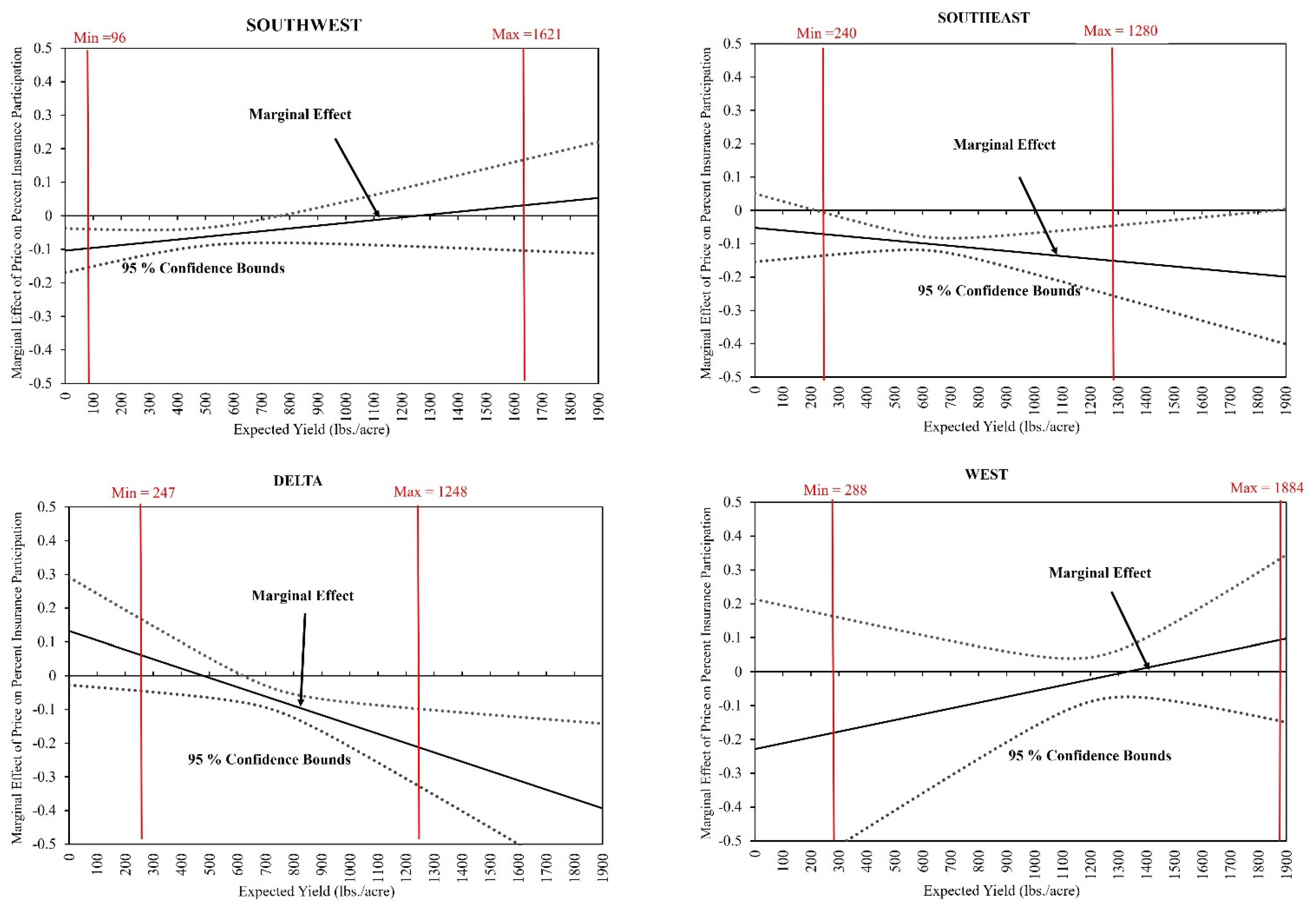
4.2. Marginal Effect of Expected Price on PINSUR Given Yield

Generally, counties that exhibited the highest cotton yields were irrigated or had the lowest production risk. Prices were also relatively higher for irrigated counties due to better overall quality. Average lint prices for the west were 79.7 US cents/lb over this period, while they were just 69.9 for the southwest. On the other hand, dryland production or counties with limited rainfall displayed relatively low yields and high production risks. The effects of cotton’s expected price (E[Pcot,it]) and yield (YLDit) plus their interaction term, E[Pcot,it]YLDit, on PINSUR and PCOTACRES were included in the model. Our model allowed us to derive marginal effects for different yield values, as shown in Figure 4, Figure 5, Figure 6 and Figure 7 (0 to 1900 with an increment of 50).
From Equation (10), we could derive the marginal effect of cotton’s expected price on PINSUR given the expected yield.
( P I N S U R ) ( E [ P c o t ] ) = ( β 1 δ 2 + β 4 ) + ( β 1 δ 4 + β 6 ) Y L D 1 β 1 δ 1 .
Considering the parameter estimates and standard errors, for the US (see Figure 4), the marginal effects of E[Pcot,it] on insurance participation suggest that an increase in expected price caused a decline in insurance participation among counties with relatively low yields. A negative sign for the marginal effect on counties with yield values less than 1700 pounds per acre indicates this fact. Lower yield counties had a more significant response compared to counties with higher yields. A similar pattern was noticeable in the southwest and west (Figure 5). The Delta region showed that higher-yield counties have a more significant response, with higher estimated magnitudes, suggesting that an increase (decrease) in expected price causes a decrease (increase) in insurance participation.
In counties where yields were relatively high, crop insurance participation declined with a high expected price because the probability of receiving indemnity payments in these counties was low. However, a low price expectation near the loan rate may have caused counties with high yields to insure more since the odds and premiums associated with prices declining were low. On the other hand, counties with very low yields behaved just the opposite. This finding is very interesting as it suggests that expected cotton revenue drives demand for crop insurance, and it also highlights regional response differences. Our results indicate that an increase in the expected subsidy per pound of production consistently led to an increase in insurance participation. In line with Keeton and Skees (1999), this finding suggests that insurance subsidies should target a dollar per unit of production rather than a percentage of the expected yield as currently formulated.

4.3. Marginal Effects of Expected Price on PCOTACRES Given Yield

Like insurance participation, we derived the marginal effect of the expected price on PCOTACRES given yield using Equation (13). The marginal effect was defined as
( P C O T A C R E S ) ( E [ P c o t ] ) = ( δ 1 β 4 + δ 2 ) + ( δ 1 β 6 + δ 4 ) Y L D 1 δ 1 β 1 .
The marginal effect of E[Pcot,it] on cotton acreage is given in Figure 6 for the US and Figure 7 for the regions. In the southeast, the marginal impact of expected price increased with yield. An increase in the expected price had a smaller impact on acreage, and there was more acreage response from counties with higher yields.
In contrast, in the US, southwest, and west, the marginal impact of price decreased when yield increased (Figure 7). This decrease may indicate that counties with very high yields were those that used irrigation and were unable to expand acreage due to limited irrigation water. Therefore, when yields were very high, an increase in price resulted in a smaller impact on acreage because the options for putting more land into production were limited. Delta estimates were negative, and the magnitude increased as expected yield increased, suggesting a more significant response from counties with high compared to low expected yields.
We also evaluated the elasticity of the percentage of cropland planted with insurance participation (Table 5). For the US, the elasticity was negative and statistically significant (−0.578), suggesting that cotton’s acreage response was inelastic to insurance participation. In line with Woodard (2015) and as suggested by Woodard (2016), our finding implies that demand for insurance could be more elastic than reported by prior studies.
The STAX program was introduced to provide additional revenue protection to cotton producers when cotton ceased to be a commodity program crop. Estimates for DCPSTAX suggest a positive impact on insurance participation, while the opposite was observed for crop acreage planted with cotton. Furthermore, our results suggest that the loss of commodity program status for cotton and STAX implementation resulted in a 5.27% decrease in the percent of acres planted with cotton for the US. As for the regions, the southwest showed the highest decline, with −5.51% of acres planted with cotton, followed by the southeast with −4.29%. DCPSTAX was not statistically significant for the Delta and the west, suggesting that STAX had very little or no impact on insured cotton acres in these two regions.

5. Conclusions

The effects of cotton insurance programs and their impact on producers’ participation and the percent of cropland planted with cotton in a county were examined for the US and each of the four major US cotton-producing regions. Using simultaneous equations for crop insurance participation and the percentage of cropland planted with cotton, we found that the effects of subsidized crop insurance were not uniform throughout the US, and substantial regional differences occurred. In line with prior studies (Deal 2004; Goodwin et al. 2004), we found that estimates of cotton acreage elasticity to insurance participation were inelastic for the US and the regions, except for the southeast. However, regional responses were not statistically significant. Our US estimated magnitude was higher than reported by Deal (2004) and Goodwin et al. (2004). Our findings suggest that crop insurance’s demand could be more elastic than previously reported by prior studies.
US counties with low yields, usually those in rainfed or dryland regions, were more responsive to insurance participation than those with very high yields as price expectations increased. Moreover, counties with very low yields responded more to changes in expected prices than counties with relatively high yields. An important policy implication of this result is that price and insurance subsidies benefit lower- more than higher-yielding counties. Furthermore, higher insurance subsidies led to greater insurance participation and cotton production in these relatively low-yielding counties. The counties in states with relatively lower yields also tended to have lower average state prices than higher-yielding states. Thus, as Keeton and Skees (1999) advocated, crop insurance subsidies would be less distorting if they targeted a per-unit subsidy rather than a percentage of the expected yield as currently structured.
Last year’s rate of return to crop insurance had a statistically significant but relatively minor impact on planted acres compared to the longer-horizon subsidy per pound expectation, calculated using the 5 year trailing yield average of a county. The estimated acreage response from insurance participation was positive and statistically significant for the southwest and negative and statistically significant for the Delta. Most of the variables were not significant for the west, suggesting that cropping decisions for irrigated acres were not affected much by crop insurance. This region also received the lowest subsidy per pound of actual production (see Table 1).
The Laspeyres revenue index of crops was considered for the top five competing crops, corn, rice, sorghum, soybeans, and wheat, in each county. However, further research is needed to develop more detailed indices at the county and regional levels that would allow quicker reactions to competing commodity crops and subsidized crop insurance. We believe the Energy Policy Act of 2005 may have contributed to the decline in the percentage of cropland planted to cotton in regions outside the west. Furthermore, crop insurance subsidies increased for all program commodities over the 1996 to 2016 period, even though STAX was unique for cotton.
Several studies investigated the effects of crop insurance on pest control inputs through chemicals and pesticides (e.g., Horowitz and Lichtenberg 1993; Smith and Goodwin 1996; Mishra et al. 2005). There is an argument for causality running from crop insurance to Bt adoption. Smith and Goodwin (1996) found that wheat producers jointly decide the amount of chemical input to use and crop insurance. Similarly, we utilized a simultaneous equation approach in looking at the relationship between crop insurance and Bt. However, an important research question would be to explore the possible two-way relationships between pest control and crop insurance and acreage planting decisions.
In the wake of climate change and more frequent extreme weather events, crop insurance programs need to become more efficient (Hazell and Varangis 2020). How crop insurance participation influences water withdrawals due to irrigation also needs to be considered. Deryugina and Konar (2017) found that a 1% increase in insured crop acreage leads to a 0.223% increase in irrigation withdrawals. More studies are needed to investigate connections among climate change, water withdrawals, premium subsidies, efficiency, and taxpayer burden (Miglietta et al. 2021; Smith 2020).

Author Contributions

Conceptualization, I.S. and R.T.; methodology, I.S. and R.T.; software, I.S.; validation, I.S. and R.T.; formal analysis, I.S. and R.T.; investigation, I.S. and R.T.; resources, R.T.; data curation, I.S. and R.T.; writing—original draft preparation, I.S.; writing—review and editing, I.S. and R.T.; visualization, I.S. and R.T. All authors read and agreed to the published version of the manuscript.

Funding

This research received no external funding.

Institutional Review Board Statement

Not applicable.

Informed Consent Statement

Not applicable.

Data Availability Statement

Data are available for replication upon request.

Acknowledgments

The authors would like to acknowledge Satheesh Aradhyula for providing valuable modeling and estimation insights.

Conflicts of Interest

The authors declare no conflict of interest.

Notes

1
This study does not include the relatively very small acreage and production of extra long staple or pima cotton, and upland cotton is subsequently referred to as cotton.
2
Monthly prices from the National Cotton Council of America (http://www.cotton.org/econ/prices/monthly.cfm) (Accessed on 5 July 2018).
3
Southeast region includes Alabama, Florida, Georgia, North Carolina, South Carolina, and Virginia; Delta region includes Arkansas, Louisiana, Mississippi, Missouri, and Tennessee; southwest region includes Kansas, Oklahoma, and Texas; west region includes Arizona, California, and New Mexico.

References

  1. Ali, Williams, Awudu Abdulai, and Ashok K. Mishra. 2020. Recent advances in the analyses of demand for agricultural insurance in developing and emerging countries. Annual Review of Resource Economics 12: 411–30. [Google Scholar] [CrossRef]
  2. Azzam, Azzeddine, Cory Walters, and Taylor Kaus. 2021. Does subsidized crop insurance affect farm industry structure? Lessons from the US. Journal of Policy Modeling. [Google Scholar] [CrossRef]
  3. Babcock, Bruce. 2011. Time to Revisit Crop Insurance Premium Subsidies? CARD Policy Briefs. p. 2. Available online: https://lib.dr.iastate.edu/card_policybriefs/2 (accessed on 7 March 2020).
  4. Baltagi, Badi H., and Young-Jae Chang. 2000. Simultaneous Equations with Incomplete Panels. Econometric Theory 16: 269–79. [Google Scholar] [CrossRef]
  5. Baltagi, Badi Hani. 2005. Econometric Analysis of Panel Data, 3rd ed. Hoboken: Wiley. [Google Scholar]
  6. Barnett, Barry, Keith Coble, Thomas Knight, Leslie Meyer, Robert Dismukes, and Jerry Skees. 2002. Impact of the Cotton Crop Insurance Program on Cotton Planted Acreage; Technical Report, Report Prepared for the Board of Directors, Federal Crop Insurance Corporation, Risk Management Agency. Washington, DC: U.S. Department of Agriculture. Available online: https://legacy.rma.usda.gov/fcic/2002/717CottonReport_RMAFCIC.pdf (accessed on 7 March 2020).
  7. Bekkerman, Anton, Eric J. Belasco, and Vincent H. Smith. 2019. Does Farm Size Matter? Distribution of Crop Insurance Subsidies and Government Program Payments across U.S. Farms. Applied Economic Perspectives and Policy 41: 498–518. [Google Scholar] [CrossRef]
  8. Coble, Keith H., Thomas O. Knight, Rulon D. Pope, and Jeffery R. Williams. 1996. Modeling Farm-Level Crop Insurance Demand with Panel Data. American Journal of Agricultural Economics 78: 439–47. [Google Scholar] [CrossRef]
  9. Cole, Shawn A., and Wentao Xiong. 2017. Agricultural insurance and economic development. Annual Review of Economics 9: 235–62. [Google Scholar] [CrossRef]
  10. Cornwell, Christopher, Peter Schmidt, and Donald Wyhowski. 1992. Simultaneous Equations and Panel Data. Journal of Econometrics 51: 151–81. [Google Scholar] [CrossRef]
  11. Dahal, Bhishma R., Sudip Adhikari, and Aditya R. Khanal. 2021. Willingness to pay for crop insurance: A case from citrus farmers in Nepal. Journal of Agribusiness in Developing and Emerging Economies. [Google Scholar] [CrossRef]
  12. Deal, John L. 2004. The Empirical Relationship Between Federally-Subsidized Crop Insurance and Soil Erosion. Ph.D. dissertation, North Carolina State University, Raleigh, NC, USA. [Google Scholar]
  13. Deryugina, Tatyana, and Megan Konar. 2017. Impacts of Crop Insurance on Water Withdrawals for Irrigation. Advances in Water Resources 110: 437–44. [Google Scholar] [CrossRef]
  14. Duffy, Patricia A., James W. Richardson, and Michael K. Wohlgenant. 1987. Regional Cotton Acreage Response. Southern Journal of Agricultural Economics 19: 99–110. [Google Scholar] [CrossRef] [Green Version]
  15. Fernandez-Cornejo, Jorge, and William D. McBride. 2002. Adoption of Bioengineered Crops. In Agricultural Economic Report. Number 810. Washington, DC: Economic Research Service/USDA. [Google Scholar] [CrossRef]
  16. Frisvold, George B., Russell Tronstad, and Jorgen Mortensen. 2000. Adoption of Bt Cotton: Regional Differences in Producer Costs and Returns. Proceedings of the Beltwide Cotton Conference 1: 337–40. [Google Scholar]
  17. Glauber, Joseph. W. 2007. Double Indemnity: Crop Insurance and the Failure of U.S. Agricultural Disaster Policy. Paper Prepared for American Enterprise Institute Project, Agricultural Policy for the 2007 Farm Bill and Beyond; Available online: https://www.aei.org/wp-content/uploads/2017/07/The-2007-Farm-Bill-and-Beyond.pdf?x91208 (accessed on 21 August 2021).
  18. Glauber, Joseph W. 2004. Crop Insurance Reconsidered. American Journal of Agricultural Economics 86: 1179–95. [Google Scholar] [CrossRef]
  19. Glauber, Joseph W., Keith J. Collins, and Peter J. Barry. 2002. Crop Insurance, Disaster Assistance, and the Role of the Federal Government in Providing Catastrophic Risk Protection. Agricultural Finance Review 62: 81–101. [Google Scholar] [CrossRef] [Green Version]
  20. Goodwin, Barry K. 1993. An Empirical Analysis of the Demand for Multiple Peril Crop Insurance. American Journal of Agricultural Economics 75: 425–34. [Google Scholar] [CrossRef]
  21. Goodwin, Barry K., and Vincent H. Smith. 2013. What Harm Is Done By Subsidizing Crop Insurance? American Journal of Agricultural Economics 95: 489–97. [Google Scholar] [CrossRef] [Green Version]
  22. Goodwin, Barry K., Monte L. Vandeveer, and John L. Deal. 2004. An Empirical Analysis of Acreage Effects of Participation in the Federal Crop Insurance Program. American Journal of Agricultural Economics 86: 1058–77. [Google Scholar] [CrossRef]
  23. Hazell, Peter B. 1992. The appropriate role of agricultural insurance in developing countries. Journal of International Development 4: 567–81. [Google Scholar] [CrossRef]
  24. Hazell, Peter, and Panos Varangis. 2020. Best practices for subsidizing agricultural insurance. Global Food Security 25: 100326. [Google Scholar] [CrossRef]
  25. Horowitz, John K., and Erik Lichtenberg. 1993. Insurance, Moral Hazard, and Chemical Use in Agriculture. American Journal of Agricultural Economics 75: 926–35. [Google Scholar] [CrossRef]
  26. Hsiao, Cheng. 2003. Analysis of Panel Data, 2nd ed. Cambridge: Cambridge University Press. [Google Scholar]
  27. Keeton, Kara, and Jerry R. Skees. 1999. The Potential Influence of Risk Management Programs on Cropping Decisions at the Extensive Margin. Master’s thesis, University of Kentucky, Lexington, KY, USA. [Google Scholar]
  28. Knisley, Shelbi R. 2016. Changes in Southern Cotton and Peanut Producing Regions. No. 333-2016-14818. Available online: https://ageconsearch.umn.edu/record/235431/ (accessed on 21 August 2021).
  29. Miglietta, Pier Paolo, Donatella Porrini, Giulio Fusco, and Fabian Capitanio. 2021. Crowding out agricultural insurance and the subsidy system in Italy: Empirical evidence of the charity hazard phenomenon. Agricultural Finance Review 81: 237–49. [Google Scholar] [CrossRef]
  30. Mishra, Ashok K., R. Wesley Nimon, and Hisham S. El-Osta. 2005. Is Moral Hazard Good for the Environment? Revenue Insurance and Chemical Input Use. Journal of Environmental Management 74: 11–20. [Google Scholar] [CrossRef]
  31. O’Donoghue, Erik. 2014. The Effects of Premium Subsidies on Demand for Crop Insurance. USDA-ERS Economic Research Report, 169. [Google Scholar] [CrossRef]
  32. Serra, Teresa, Barry K. Goodwin, and Allen M. Featherstone. 2003. Modeling Changes in the U.S. Demand for Crop Insurance during the 1990s. Agricultural Finance Review 63: 109–25. [Google Scholar] [CrossRef] [Green Version]
  33. Shaik, Saleem, Keith H. Coble, Thomas O. Knight, Alan E. Baquet, and George F. Patrick. 2008. Crop Revenue and Yield Insurance Demand: A Subjective Probability Approach. Journal of Agricultural and Applied Economics 40: 757–66. [Google Scholar] [CrossRef] [Green Version]
  34. Smith, Vincent H. 2020. The US federal crop insurance program: A case study in rent seeking. Agricultural Finance Review 80: 339–58. [Google Scholar] [CrossRef]
  35. Smith, Vincent H., and Barry K. Goodwin. 1996. Crop Insurance, Moral Hazard, and Agricultural Chemical Use. American Journal of Agricultural Economics 78: 428–38. [Google Scholar] [CrossRef]
  36. USDA. 2017a. National Agricultural Statistics Service (NASS), 1985 to 2016. Quick Stats 1.0, State and County Data. Online. Available online: http://www.nass.usda.gov/ (accessed on 15 December 2017).
  37. USDA. 2017b. Risk Management Agency (RMA), 1995 to 2016. Summary of Business Online and Online Premium Calculator. Online. Available online: http://www.rma.usda.gov/ (accessed on 9 May 2017).
  38. USDA. 2018. Agricultural Marketing Service (AMS), (Various Issues). Cotton Market News. Online. Available online: http://www.marketnews.usda.gov/portal/cn (accessed on 5 January 2018).
  39. Vandeveer, Monte L., and C. Edwin Young. 2001. The Effects of the Federal Crop Insurance Program on Wheat Acreage; Economic Research Service. Washington, DC: U.S. Department of Agriculture, pp. 21–30.
  40. Williams, Michael R. 1995–2016. Cotton Insect Loss Estimates, Proceedings of the Beltwide Cotton Conferences. Online. Available online: http://www.entomology.msstate.edu/resources/tips/cotton-losses/data/ (accessed on 26 December 2018).
  41. Woodard, Joshua D. 2015. Estimating Demand for Government Subsidized Insurance: Evidence from the U.S. Agricultural Insurance Market. Available online: https://papers.ssrn.com/sol3/papers.cfm?abstract_id=2826036 (accessed on 21 August 2021).
  42. Woodard, Joshua D. 2016. Crop Insurance Demand More Elastic than Previously Thought. Choices, 31. Available online: https://www.jstor.org/stable/choices.31.3.15 (accessed on 21 August 2021).
  43. Wu, Junjie, and Richard M. Adams. 2001. Production Risk, Acreage Decisions and Implications for Revenue Insurance Programs. Canadian Journal of Agricultural Economics/Revue Canadienne d’agroeconomie 49: 19–35. [Google Scholar] [CrossRef]
  44. Wu, Junjie. 1999. Crop Insurance, Acreage Decisions, and Nonpoint-Source Pollution. American Journal of Agricultural Economics 81: 305–20. [Google Scholar] [CrossRef]
  45. Young, C. Edwin, Monte L. Vandeveer, and Randall D. Schnepf. 2001. Production and Price Impacts of U.S. Crop Insurance Programs. American Journal of Agricultural Economics 83: 1196–203. [Google Scholar] [CrossRef]
  46. Yu, Jisang, Aaron Smith, and Daniel A. Sumner. 2018. Effects of Crop Insurance Premium Subsidies on Crop Acreage. American Journal of Agricultural Economics 100: 91–114. [Google Scholar] [CrossRef] [Green Version]
  47. Zahid, Zobia, Muhammad Kashif Riaz Khan, Amjad Hameed, Muhammad Akhtar, Allah Ditta, Hafiz Mumtaz Hassan, and Ghulam Farid. 2021. Dissection of Drought Tolerance in Upland Cotton through Morpho-Physiological and Biochemical Traits at Seedling Stage. Frontiers in Plant Science 12: 260. [Google Scholar] [CrossRef] [PubMed]
Figure 1. Expected premium subsidy per pound of production (SUBSIDYPERLB) and acres of upland cotton planted for California and Texas, 1996–2016.
Jrfm 14 00562 g001
Figure 2. Insured US upland cotton acreage by coverage types, 1996–2016.
Jrfm 14 00562 g002
Figure 3. Insured US upland cotton acreage by coverage level and region, 1996–2016.
Jrfm 14 00562 g003
Figure 4. Marginal effect of expected price on insurance participation given expected yield for US.
Jrfm 14 00562 g004
Figure 5. Marginal effects (by region) of expected price on insurance participation given expected yields.
Jrfm 14 00562 g005
Figure 6. US marginal effect of expected price on the percentage of cotton planted given expected yield.
Jrfm 14 00562 g006
Figure 7. Marginal effects (by region) of expected price on the percentage of cotton planted given expected yields.
Jrfm 14 00562 g007
Table 1. US and regional county summary statistics.
Region
# of Observations
DeltaSoutheastSouthwestWestUS
1647403633104799472
Dependent variables
PINSURit0.432 *0.5690.5400.3780.525
(0.203)(0.221)(0.236)(0.192)(0.230)
PCOTACRESit0.1460.1940.1750.1020.174
(0.123)(0.150)(0.204)(0.106)(0.167)
Independent variables
SUBSIDYPERLBit0.0240.0420.0540.0160.042
(0.016)(0.024)(0.036)(0.018)(0.030)
PRORit−12.5872.5722.8212.4892.657
(8.47)(8.708)(5.733)(5.405)(7.599)
E[Picot,it]0.7390.7460.6990.7970.731
(0.187)(0.191)(0.171)(0.195)(0.186)
YLDit−58036905831146695
(162)(141.56)(238)(293)(232.20)
E[Picot,it] YLDit−5591.3515.9409.3925512.4
(177.8)(166.9)(195.7)(356)(224.7)
YLDVARit0.1840.2380.2740.1630.237
(0.066)(0.075)(0.107)(0.074)(0.093)
PBTit0.7930.7570.5110.3920.659
(0.249)(0.249)(0.357)(0.366)(0.327)
RREVINDEXit0.9310.8820.8790.5880.874
(0.532)(0.655)(0.614)(0.753)(0.630)
DCPSTAX0.1250.1140.1320.0610.120
(0.331)(0.318)(0.339)(0.239)(0.324)
Other descriptors
Cotton planted acres28,10913,92439,25824,10825,793
(35,373)(14,103)(64,098)(38,909)(44,0043)
Total cropland acres176,10769,096205,664298,672147,406
(107,082)(39,400)(117,083)(286,862)(129,758)
Cotton insured acres24,92613,11637,62720,23624,124
(31,507)(13,485)(62,903)(33,790)(42,511)
* Mean values are above the sample standard errors in parentheses.
Table 2. (a) Parameter estimates of simultaneous equations: percent insurance participation. (b) Parameter estimates of simultaneous equations: percent cotton planted.
Dependent VariableDelta
N = 1647
Southeast
N = 4036
Southwest
N = 3310
West
N = 479
US
N = 9472
(a)
Intercept−0.01149 ***
(0.00393)
−0.00691 ***
(0.00260)
−0.01238 ***
(0.00257)
0.05273
(0.16149)
−0.00934 ***
(0.00148)
E[Pcot,it]0.15539
(0.10641)
−0.13886 **
(0.06594)
−0.08703 **
(0.03448)
0.58585
(2.50084)
−0.12282 ***
(0.02244)
YLDit0.00011
(0.00013)
−0.00005
(0.00008)
−0.00011 **
(0.00006)
−0.00141
(0.00397)
−0.00011 ***
(0.00003)
E[Pcot,it] YLDit−0.00011
(0.00015)
0.00003
(0.00010)
0.00002
(0.00006)
−0.00083
(0.00292)
0.00001
(0.00004)
YLDVARit0.28717 ***
(0.10550)
−0.01962
(0.04601)
0.04862
(0.03303)
−0.78313
(2.02821)
−0.00262
(0.02377)
PBTit0.44285 ***
(0.03964)
0.17829 ***
(0.03109)
0.12766 ***
(0.01092)
−0.00705
(0.25789)
0.17402 ***
(0.00794)
SUBSIDYPERLBit7.00171 ***
(0.50352)
4.84789 ***
(0.13402)
4.46006 ***
(0.15390)
5.31541
(4.08394)
4.64178 ***
(0.07636)
PRORit−10.00110 **
(0.00046)
0.00019
(0.00023)
0.00174 ***
(0.00041)
0.00109
(0.01892)
0.00056 ***
(0.00018)
PCOTACRESit1.33629 ***
(0.46835)
−1.47798 **
(0.43738)
−0.72529 ***
(0.26162)
−0.16851
(0.45524)
−0.86598 ***
(0.14083)
DCPSTAX0.23648 ***
(0.02355)
0.16246 ***
(0.01849)
0.16775 ***
(0.01289)
−0.22387
(0.95475)
0.16242 ***
(0.00785)
Dependent VariableDelta
N = 1647
Southeast
N = 4036
Southwest
N = 3310
West
N = 479
US
N = 9472
(b)
Intercept0.00046
(0.00170)
0.00330 ***
(0.00097)
0.00521 ***
(0.00098)
0.00338 *
(0.00205)
0.00459 ***
(0.00065)
E[Pcot,it]−0.00031
(0.04544)
−0.05774 **
(0.02538)
0.03337 **
(0.01380)
0.04546
(0.04609)
0.03567 ***
(0.01045)
YLDit−0.00010 **
(0.00005)
−0.00003
(0.00003)
0.00010 ***
(0.00002)
−0.00009 **
(0.00004)
0.00004 ***
(0.00001)
E[Pcot,it] YLDit−0.00016 **
(0.00006)
0.00007 *
(0.00004)
−0.00009 ***
(0.00002)
−0.00006
(0.00004)
−0.00009 ***
(0.00002)
YLDVARit−0.13778 ***
(0.03577)
−0.00592
(0.01933)
−0.02849 **
(0.01294)
−0.04260
(0.05027)
−0.02827 ***
(0.01088)
PBTit−0.02148 *
(0.01231)
−0.07045 ***
(0.00691)
−0.03280 ***
(0.00467)
−0.00128
(0.01213)
−0.04505 ***
(0.00379)
RREVINDEXit−0.02136 ***
(0.00362)
−0.00882 ***
(0.00161)
−0.01737 ***
(0.00168)
0.00122
(0.00370)
−0.01734 ***
(0.00110)
PINSURit−0.12811 ***
(0.02148)
0.01896
(0.01204)
0.09890 ***
(0.00959)
−0.01256
(0.03013)
0.04981 ***
(0.00744)
DCPSTAX−0.01922 ***
(0.00829)
−0.04298 ***
(0.00512)
−0.05513 ***
(0.00444)
−0.01928
(0.01397)
−0.05271 ***
(0.00315)
Notes: Numbers in parentheses are estimated standard errors. Single, double, and triple asterisks (*, **, and ***) indicate statistical significance at the 10%, 5%, and 1% levels.
Table 3. (a) Marginal effects on insurance participation (PINSUR). (b) Marginal effects on percent cotton planted (PCOTACRES).
Dependent VariableDelta
N = 1647
Southeast
N = 4036
Southwest
N = 3310
West
N = 479
US
N = 9472
(a)
YLDVARit0.08800
(0.06370)
−0.01057
(0.03989)
0.06465
(0.03204)
−0.08285
(0.23871)
0.02096
(0.02290)
PBTit0.35361 ***
(0.0166)
0.27472 ***
(0.00994)
0.14131 ***
(0.00979)
0.01850
(0.05152)
0.20422 ***
(0.00618)
REVINDEXit−0.02437 ***
(0.00658)
0.01268 **
(0.00326)
0.01176 ***
(0.00417)
−0.02611 *
(0.01367)
0.01440 ***
(0.00228)
SUBSIDYPERLBit5.97826 ***
(0.22813)
4.71577 ***
(0.11708)
4.16154 ***
(0.09933)
6.74184 ***
(1.93728)
4.44985 ***
(0.06970)
PRORit−10.00094 **
(0.00037)
0.00018
(0.00022)
0.00162 ***
(0.00039)
0.00138
(0.02310)
0.00054 ***
(0.00017)
PCOTACRESit1.33629 ***
(0.46835)
−1.47798 ***
(0.43738)
−0.72529 ***
(0.26162)
−16.85069
(45.52391)
−0.86598 ***
(0.14083)
Dependent VariableDelta
N = 1647
Southeast
N = 4036
Southwest
N = 3310
West
N = 479
US
N = 9472
(b)
YLDVARit−0.14905 ***
(0.03554)
−0.00612
(0.01922)
−0.02210 *
(0.01235)
−0.04156
(0.04974)
−0.02723 ***
(0.01067)
PBTit−6.67858 ***
(0.92518)
−0.06524 ***
(0.00479)
−0.01882 ***
(0.00377)
−0.00152
(0.01166)
−0.03487 ***
(0.00288)
REVINDEXit−0.01824 ***
(0.00367)
−0.00858 ***
(0.00157)
−0.01621 ***
(0.00160)
0.00155
(0.00360)
−0.01662 ***
(0.00106)
SUBSIDYPERLBit−0.76589 ***
(0.12744)
0.08939
(0.05643)
0.41159 ***
(0.03790)
−0.08465
(0.19900)
0.22163 ***
(0.03245)
PRORit−1−0.00012 **
(0.00005)
0.000003
(0.000005)
0.00016 ***
(0.00004)
−0.00002
(0.00030)
0.00003 ***
(0.00001)
PINSURit−0.12811 ***
(0.02148)
0.01896
(0.01204)
0.09890 ***
(0.00959)
−0.01256
(0.03013)
0.04981 ***
(0.00744)
Notes: Numbers in parentheses are estimated standard errors. Single, double, and triple asterisks (*, **, and ***) indicate statistical significance at the 10%, 5%, and 1% levels.
Table 4. US and regional county planted acreage response estimates (acres).
DeltaSoutheastSouthwestWestUS
YLDVARit−26,249 ***
(6259)
−423
(1328)
−4545 *
(2540)
−12,716
(15,219)
−4013 ***
(1573)
PBTit−11,761 ***
(1629)
−4508 ***
(331)
−3872 ***
(776)
−464
(3569)
−5141 ***
(425)
RREVINDEXit−3212 ***
(646)
−593 ***
(108)
−3333 ***
(329)
474
(1102)
−2451 ***
(157)
SUBSIDYPERLBit($/lb)−134,878 ***
(22,442)
6177
(3899)
84,649 ***
(7795)
−25,902
(60,890)
32,669 ***
(4783)
PRORit−1−21.25 **
(9.19)
0.24
(0.33)
33.00 ***
(8.48)
−5.31
(91.35)
3.94 ***
(1.38)
Notes: Numbers in parentheses are estimated standard errors. Single, double, and triple asterisks (*, **, and ***) indicate statistical significance at the 10%, 5%, and 1% levels.
Table 5. Elasticity of percentage of cropland planted to insurance participation.
DeltaSoutheastSouthwestWestUS
EPCOTACRES/PINSUR−0.39021
(1.02424)
3.29876
(3.74565)
−0.68339
(0.42661)
−0.78285
(1.12306)
−0.57759 ***
(0.21159)
Notes: Numbers in parentheses are estimated standard errors. Single, double, and triple asterisks. *** indicate statistical significance at the 1% level.
Publisher’s Note: MDPI stays neutral with regard to jurisdictional claims in published maps and institutional affiliations.

