Abstract
Prior theory suggests a positive relation between volatility and market depth, while past empirical research finds contrasting results. This paper examines the relation between the volatility and the limit order book depth in commodity and foreign exchange futures markets during a turbulent time using the generalized method of moments (GMM). Results indicate a negative relation between volatility and depth and suggest that the depth in the limit order book decreases as volatility increases. Findings help to understand how market participants provide liquidity in response to shifts in prices.
1. Introduction
In markets with limit order books, limit orders provide liquidity and market orders expend it. As a result, limit orders perform an essential role in the provision of liquidity. One crucial aspect of liquidity provision is the role of volatility. This study examines the interaction between volatility and order-flow composition motivated by the theories presented in Handa and Schwartz (1996) and Foucault (1999). Handa and Schwartz (1996) develop a model in which investors decide to place market or limit orders. This decision is influenced by investors’ beliefs about the likelihood of order execution against a liquidity trader versus an informed trader. According to Handa and Schwartz (1996), investors place more limit orders than market orders when price volatility is elevated. Trading against liquidity traders yields a higher expected gain than the expected loss trading against informed traders.
Furthermore, Foucault (1999) demonstrates that as volatility rises, the submission of market orders becomes more expensive, and thus more limit orders are placed. The implication is that as volatility increases, so does the number of limit orders placed. When volatility rises, the models of Handa and Schwartz (1996) and Foucault (1999) predict an increase in the number of limit orders placed. As a result, if more limit orders are submitted, the available depth should also rise.
This paper examines the relation between volatility and the limit order book depth in a U.S. electronic, order-driven futures market. This study contributes to the literature in several ways. First, we employ actively traded futures contracts on commodities and foreign exchange. Prior research that examines the volatility-depth relation focuses on equity markets (Ahn et al. 2001; Vo 2007) and market index futures (Chen and Wu 2009; Chiang et al. 2009). Aidov and Daigler (2015) show that depth characteristics in the limit order book in futures markets contrast with those in equity markets. In addition, Bryant and Haigh (2004) suggest that commodity futures markets possess intrinsically different liquidity attributes than financial futures markets and warrant separate examination. Second, we use a high-frequency sampling method to construct our depth variables. In contrast to prior studies, which sample depth at the end of a time interval, we sample depth within time intervals using the first depth update in each second. Depth fluctuates throughout the day and certainly within intervals, and our sampling procedure allows for the capture of average depth variations within intervals. Third, the prior literature that examines volatility and depth finds opposite results (e.g., Ahn et al. 2001; Chen and Wu 2009). We provide further evidence on this topic. Finally, we examine a market setting during a turbulent period centering on the financial crisis of 2008. Prior research finds that market participants withdraw depth from the limit order book during extreme market movements (Goldstein and Kavajecz 2004). In contrast, Locke and Sarkar (2001) imply that electronic markets with limit order books may not suffer liquidity crashes during periods of high volatility. The period we examine allows us to explore the relation between volatility and limit order book depth during crisis events.
Our results support an inverse relation between volatility and subsequent market depth for several depth proxies and across a set of volatility measures. Results are robust to adjustment for control factors. Finally, we find a similar negative relation after adjusting for structural breaks in positive and negative trending subperiods. The paper is organized as follows. Section 2 describes the related literature. Section 3 presents the data and methodology. Results are discussed in Section 4. Section 5 offers concluding remarks.
2. Literature Review
This paper relates to the literature that studies the provision of liquidity in limit order books. Biais et al. (1995) show that the conditional probability that traders place limit orders is larger when there is a lack of liquidity. Fishe et al. (2021) support the notion that limit order traders delay providing liquidity during active markets. Furthermore, both Kavajecz (1999) and Smales (2019) find that liquidity is removed from the market around information events.
Literature that examines the interaction of liquidity and volatility in limit order books is also related to our study. Locke and Sarkar (2001) find that liquidity does not increase with volatility in futures markets. Næs and Skjeltorp (2006) show that volatility is negatively related to the limit order book slope for equities on the Oslo Stock Exchange (OSE). Tian et al. (2019) find that the limit order book slope for oil futures decreases when volatility is expected to increase.
This article is related to research that investigates the relationship between volatility and market depth. Open interest is used as a proxy for market depth in the early work on the volatility-depth relation. Bessembinder and Seguin (1993) use eight futures contracts to show that volatility and open interest are inversely related. In addition, Fung and Patterson (2001) establish an inverse relation between volatility and open interest for a set of foreign exchange and interest rate futures contracts.
One of the first research papers to analyze the relation between volatility and depth using actual depth data is Ahn et al. (2001). They examine the intraday volatility-depth relation for companies listed on the Stock Exchange of Hong Kong (SEHK), using the number of limit orders in the five-deep limit order book. After adjusting for transaction frequency, intraday market depth variation, and market depth autocorrelation, they conclude that an increase in volatility results in an increase in market depth. Vo (2007) documents contradictory findings indicating that price volatility is negatively associated with market depth for Toronto Stock Exchange (TSE) traded equities.
Chiang et al. (2009) investigate the relation between volatility and depth for Taiwan Futures Exchange (TAIFEX) contracts. Their results demonstrate a positive but not statistically significant relationship between volatility and depth from 2002 to 2003. They further segment the futures data into bull and bear markets and observe a positive and statistically significant volatility-depth relation during bull markets but a negative relation during bear markets. Conversely, Chen and Wu (2009) show that an increase in volatility is followed by a drop in depth (quantity of limit orders across five levels) for TAIFEX futures contracts.
Overall, the past research concerning the effect of volatility on market depth for stocks and index futures finds mixed results. The relation between volatility and depth using data for foreign exchange and commodity futures markets is an unexplored topic.
3. Data and Methodology
3.1. Data
We employ three electronically traded futures contracts in this study to examine the effect of volatility on depth. Specifically, the futures contracts we consider include EUR/ USD, gold, and corn futures. For ease of exposition, the EUR/USD foreign exchange futures contract hereafter is referred to as the “EUR” futures contract. The EUR futures contract has a ticker symbol of 6E, a contract size of EUR 125,000, and is quoted in USD and cents. The gold futures contract has a ticker symbol of GC, a contract size of 100 troy ounces, and is quoted in USD and cents per troy ounce. The corn futures contract has a ticker symbol of ZC, a contract size of 5000 bushels, and is quoted in USD and cents per bushel. The EUR futures, gold futures, and corn futures trade on the Chicago Mercantile Exchange (CME), Commodity exchange (COMEX), and Chicago Board of Trade (CBOT), respectively.
The data in this paper is provided by the CME Group and is obtained from the CME Globex electronic trading system. The data is encoded in RLC format and contains all the message traffic required to reconstruct the five-deep limit order book. The data covers 2 January 2008 to 2 October 2009, for EUR futures, 1 January 2008 to 18 April 2009, for gold futures, and 11 January 2008 to 21 March 2009, for corn futures. The date range for each contract is limited by the data provided to us by the CME Group. The last date of data availability for each futures contract in this study is based on a change of data format. After the change in format from RLC to FIX/Fast format, limit order book messages are no longer recorded in the RLC format available in the database used in this study, hence the reason for the different ending dates.
Holidays and days with missing data are deleted from the sample. The daily trading hours are derived from the traditional open-outcry period, which runs from 07:20 a.m. to 2:00 p.m. Central Time for EUR futures, 07:20 a.m. to 12:30 p.m. Central Time for gold futures, and 09:30 a.m. to 01:15 p.m. Central Time for corn futures. We partition the trading hours for each futures contract into fifteen-minute intervals, as in Ahn et al. (2001). The futures contracts are rolled over when trading volume in a deferred expiration exceeds the trading volume in the near-term expiration.
3.2. Methodology
3.2.1. Variables
The variables that are used in the analysis are detailed in this section. Two depth metrics are utilized, similar to Chiang et al. (2009). The first depth measure is known as “depth quantity,” and it is defined as the sum of the depths in the limit order book’s five levels. The second depth metric is termed “depth frequency” and is calculated as the sum of the number of limit orders over the five depth levels. Arzandeh and Frank (2019) suggest that traders in electronic futures markets actively employ limit orders at price levels beyond the best (first level). As a result, for both depth measures, the full five-deep limit order book is used. Depth is sampled at the beginning of each second and averaged over fifteen-minute time intervals. In addition, the Phillips–Perron and the Ng and Perron unit root tests are used to check for unit roots in the depth measures. For all contracts, we find evidence to reject the null hypothesis of a unit root.
Three volatility measures are specified to assure that results are not dependent on any one measure of volatility. The first measure of volatility is the Garman–Klass volatility (GK volatility) measure proposed by Garman and Klass (1980). The GK volatility measure is calculated as follows:
where High denotes the highest trading price, Low denotes the lowest trade price, Open denotes the first trade price, and Close denotes the last transaction price within a fifteen-minute interval. The GK volatility estimator is approximately eight times more efficient than the classic close-to-close volatility estimator (Daigler and Wiley 1999). Będowska-Sójka and Kliber (2021) and Molnár (2012) find the Garman–Klass measure to be the best volatility estimator compared to other estimators. The GK volatility measures the volatility within a time interval and does not necessarily increase with more trades in an interval. This estimator is often employed in financial markets to study volatility (Tan et al. 2020; Batten and Lucey 2010).
The Returns volatility is the second measure of volatility that is employed. The Returns Volatility is used in previous studies, including Gwilym et al. (1999), and is computed as follows:
where Pricet is the final trade price in a fifteen-minute time interval t and Pricet−1 is the previous interval’s last price. For the opening interval of the day, Pricet is the interval’s last trade price, and Pricet−1 is the interval’s first trade price. Unlike the GK volatility measure, which calculates volatility within time intervals, the Returns volatility measure calculates volatility between time intervals. Furthermore, the Returns volatility considers a single (last) price within a time interval. Returns volatility is also commonly referred to as absolute returns.
The third volatility proxy is realized volatility, which is described in Ahn et al. (2001). The Realized volatility is calculated as follows:
where Ri,t denotes the return for the ith trade in a fifteen-minute time interval t, and N is the total number of transactions during the interval. The returns are determined as the log difference between the prices of sequential trades within a time interval. The sum of the squared returns within a fifteen-minute time period is not divided by the number of transactions because the aggregate price variations are of interest. The three volatility measures are calculated in distinct ways and consequently may offer varying results. Volatility measures are calculated based on partitioned fifteen-minute time intervals. To deal with outliers, we winsorize the three volatility measures at the 1% and 99% levels.
Similar to Ahn et al. (2001), we implicitly assume that our volatility measures are transitory. It is important to distinguish permanent volatility from transitory volatility. For example, Hendershott and Menkveld (2014) decompose price changes into a permanent component and a transitory component using a state space approach. Permanent or fundamental volatility is caused by information and occurs when there is uncertainty about fundamental security values. Transitory volatility is the propensity of prices to move around their fundamental values and is caused by liquidity trading and noise.
3.2.2. Hypotheses
The research hypotheses based on theoretical considerations are provided in this section. The research hypotheses investigated in this study are motivated by the models of Handa and Schwartz (1996) and Foucault (1999). When price volatility is high, Handa and Schwartz (1996) show that investors submit more limit orders than market orders. Foucault (1999) demonstrates that as volatility increases, the cost of submitting market orders increases, and hence more limit orders are submitted. These models serve as the basis for the following hypotheses about volatility and depth:
Hypothesis 1.
A positive relation exists between volatility and depth quantity.
Hypothesis 2.
A positive relation exists between volatility and depth frequency.
To examine these two hypotheses, the following regressions are estimated using the generalized method of moments (GMM) introduced in Hansen (1982):
The GMM methodology is an estimation technique used in many studies that examine the intraday characteristics of liquidity (Box et al. 2021; Ben Ammar and Hellara 2021; Ozturk et al. 2017). Using the Newey and West (1987) approach, the calculated t-statistics are adjusted for heteroskedasticity and autocorrelation. A positive (negative) and statistically significant coefficient on volatility indicates a positive (negative) relation between volatility and depth.
According to Ahn et al. (2001), various control variables should be included in the analysis of volatility and depth. These variables include the frequency of trades, intraday time dummy variables, and lagged depth. It is necessary to add the frequency of trades as a control variable since the realized volatility measure is positively correlated with the number of trades made in a given time interval. Additionally, time dummies and lagged depths are incorporated to account for intraday fluctuation and market depth autocorrelation. The following are the expanded models with control variables:
where Volatilityt−1 represents lagged volatility, Frequencyt corresponds to the number of trades within an interval, Volumet denotes the sum of traded volume within an interval, Deptht−1 denotes lagged depth, and the Di variables denote dummy variables that take the value one during the first and last half hours of trading and zero otherwise.
4. Results and Discussion
4.1. Summary Statistics
The summary statistics for the three futures contracts are provided in Table 1. Panels A, B, and C summarize the Depth quantity, Depth frequency, GK volatility, Returns volatility, and Realized volatility for the EUR, gold, and corn contracts, respectively.

Table 1.
Summary statistics of depth and volatility. This table presents the summary statistics of the depth and volatility measures for the fifteen-minute time intervals averaged over the sample period. Depth quantity is calculated as the sum of the depth available across all five levels in the limit order book. Depth frequency is calculated as the sum of the number of orders available across all five levels in the limit order book. GK volatility is the Garman and Klass (1980) volatility measure composed of the high, low, open, and close values in an interval. Returns volatility is calculated as the absolute value of returns across intervals. Realized volatility is the sum of squared returns in each interval.
The EUR futures possess the largest average depth (639.35) and the largest number of orders (187.63) per fifteen-minute interval. Gold futures have the smallest mean Depth quantity (105.35) and Depth frequency (50.10). According to the GK Volatility (27.66) and Returns volatility (3.51), the most volatile contract is corn. The EUR futures contract has the largest Realized volatility (142.77). The median values of the three volatility measures are all larger for the corn futures relative to the EUR and gold futures. Based on the moments presented in Table 1, the depth and volatility measures have different distributions across the contracts.
Figure 1 displays the intraday behavior of the depth and volatility measures presented in Table 1. Both depth measures for the EUR futures contract in Panel A increase at the open of the trading day and then decrease across the day. The Depth quantity for gold in Panel A and corn in Panel E increases at the open, declines over the day, and increases again at the close of trading. The Depth frequency for gold and corn futures increases near the open, declines over the middle of the day, and decreases at the end of the trading day. For the EUR futures in Panel B and the gold futures in panel D, all three volatility measures decline over the trading day. In contrast, the GK volatility, Realized volatility, and Returns volatility exhibit a U-shaped intraday pattern for the corn futures contract.
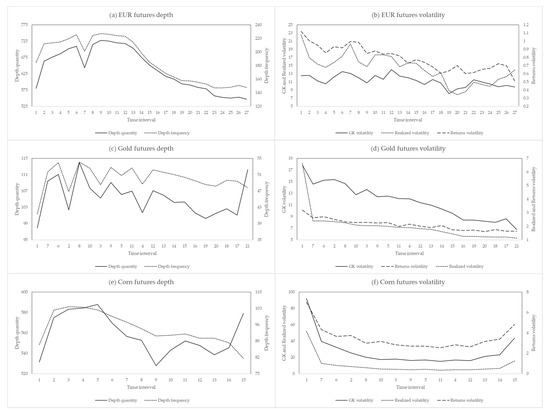
Figure 1.
The intraday depth and volatility behavior. This figure presents the intraday behavior of the depth and volatility measures over the day using 15-min time intervals. (a) depicts EUR futures depth, (b) depicts EUR futures volatility, (c) depicts Gold futures depth, (d) depicts Gold futures volatility, (e) depicts Corn futures depth, and (f) depicts Corn futures volatility. Depth quantity is calculated as the sum of the depth available across all five levels in the limit order book. Depth frequency is calculated as the sum of the number of orders available across all five levels in the limit order book. GK volatility is the Garman and Klass (1980) volatility measure composed of the high, low, open, and close values in an interval. Returns volatility is calculated as the absolute value of returns across intervals. Realized volatility is the sum of squared returns in each interval. In this figure, the Realized volatility is divided by 10 to adjust for scale.
4.2. Volatility and Depth
The next set of tables presents the results for the relation between volatility and depth using the base regressions. Table 2 presents results for the Depth quantity.
Table 2.
Volatility and depth quantity. This table presents the coefficient estimates for the following model: Depth quantity is computed as the summation of the depths available across a limit order book’s five levels. Volatility is one of three measures of volatility. GK volatility is the Garman and Klass (1980) measure of volatility that consists of the high, low, open, and close price values within an interval. Returns volatility is defined as the absolute value of returns across time intervals. Realized volatility is the summation of each interval’s squared returns. The generalized method of moments (GMM) procedure is used to estimate each regression, along with the Newey and West (1987) correction. The notation * indicates significance at the 1% level.
In Panel A, a negative and statistically significant coefficient occurs on each of the three volatility measures for the EUR futures contracts. This implies a negative or inverse relation between volatility and Depth quantity. The coefficient on GK volatility and Returns volatility is also negative and significant for the gold futures in Panel B, which also reconfirms the inverse relation. A similar result is found for the corn futures in Panel C. Table 3 presents results for the relation between volatility and Depth frequency.
Table 3.
Volatility and depth frequency. This table presents the coefficient estimates for the following model: . Depth frequency is computed as the summation of the number of orders available across a limit order book’s five levels. Volatility is one of three measures of volatility. GK volatility is the Garman and Klass (1980) measure of volatility that consists of the high, low, open, and close price values within an interval. Returns volatility is defined as the absolute value of returns across time intervals. Realized volatility is the summation of each interval’s squared returns. The generalized method of moments (GMM) procedure is used to estimate each regression, along with the Newey and West (1987) correction. The notation * indicates significance at the 1% level.
In Panel A, the relation between the GK volatility, Returns volatility, and Realized volatility, and Depth frequency is negative and statistically significant at the one percent level for the EUR futures contract. In Panel B, the relation between the three volatility measures and depth frequency is negative, as indicated by the negative and statistically significant coefficients on the volatility measures. Corn futures in Panel C also show an inverse relation between GK volatility and Returns volatility, and Depth frequency. The overall results from Table 2 and Table 3 suggest an inverse or negative relation between volatility and depth for the three volatility measures. The main implication is that a decrease in volatility in one period leads to an increase in depth in the following period.
4.3. Volatility and Depth with Control Factors
The next set of results is for the expanded models that explore the relation between volatility and depth, with the addition of control variables. Table 4 presents results for the Depth quantity.
Table 4.
Volatility and depth quantity with controls. This table shows the coefficient estimates for the following model: . Depth quantity is computed as the summation of the depths available across a limit order book’s five levels. Volatility is one of three measures of volatility. GK volatility is the Garman and Klass (1980) measure of volatility that consists of the high, low, open, and close price values within an interval. Returns volatility is defined as the absolute value of returns across time intervals. Realized volatility is the summation of each interval’s squared returns. Volume is calculated as the sum of each time interval’s trade volume. D is a dummy variable that has a value of one for the first two and last two time intervals of each day and a value of zero for the remaining time intervals. The T subscript denotes the last interval in a day. The generalized method of moments (GMM) procedure is used to estimate each regression, along with the Newey and West (1987) correction. The notations *, **, and *** indicate significance at the 1%, 5%, and 10% levels, respectively.
The main variable of interest is the coefficient (β1) on the volatility measures, which gauges the effect of volatility on market depth. For the EUR contract in Panel A, we find a negative relation between both GK and Returns volatility, and Depth quantity. In Panel B, the coefficient on GK volatility, Returns volatility, and Realized volatility is negative and statistically significant for the gold futures contract. Corn futures in Panel C also exhibit an inverse relation between GK and Returns volatility and Depth quantity. In Table 5, results for Depth frequency are presented.
Table 5.
Volatility and depth frequency with controls. This table presents the coefficient estimates for the following model: . Depth frequency is computed as the summation of the number of orders available across a limit order book’s five levels. Volatility is one of three measures of volatility. GK volatility is the Garman and Klass (1980) measure of volatility that consists of the high, low, open, and close price values within an interval. Returns volatility is defined as the absolute value of returns across time intervals. Realized volatility is the summation of each interval’s squared returns. Frequency is calculated as the number of trades in each time interval. D is a dummy variable that has a value of one for the first two and last two time intervals of each day and a value of zero for the remaining time intervals. The T subscript denotes the last interval in a day. The generalized method of moments (GMM) procedure is used to estimate each regression, along with the Newey and West (1987) correction. The notations *, **, and *** indicate significance at the 1%, 5%, and 10% levels, respectively.
The coefficient on GK volatility and Returns volatility across Panel A for the EUR and Panel B for the gold futures contract is negative and statistically significant. In Panel C, the corn futures contract exhibits an inverse relation between Returns volatility and Depth frequency as indicated by the negative coefficient β1. The significant coefficients on the intraday dummy variables across the three panels suggest the importance of adjusting for the time-of-day effect in market depth. Overall, after accounting for control factors, the results show evidence consistent with a negative relation between volatility and depth.
4.4. Structural Breaks
We note that our data encompasses a very volatile time period in financial markets. Figure 2 shows the daily mean Depth quantity and Depth frequency measures. The daily patterns of Depth quantity and Depth frequency appear to move in tandem. However, significant changes in the depth measures are evident at different points in the time period.
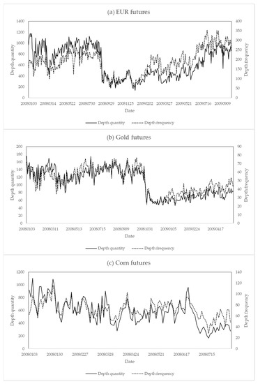
Figure 2.
Daily depth. This figure presents the daily depth for each futures contract. (a) depicts EUR futures, (b) depicts Gold futures, and (c) depicts Corn futures. Intraday depth measures are averaged over the day using fifteen-minute time interval data. Depth quantity is calculated as the sum of the depth available across all five levels in the limit order book. Depth frequency is calculated as the sum of the number of orders available across all five levels in the limit order book.
To identify subperiods with different trends, we employ the methodology of Bai and Perron (2003) to test for multiple structural breaks. For both depth measures, we establish five structural breaks at the daily time scale. Using the structural breaks as endpoints for each subperiod, we identify subperiods for the depth variables with a positive or a negative trend. A dummy variable (Break) is introduced that takes a value of one for subperiods with a positive trend in depth and a value of zero for subperiods with a negative trend in depth. This methodology is motivated by Chiang et al. (2009), who find an asymmetric relation for volatility and depth in bull and bear market subperiods. Depth regressions are estimated with the addition of the Break dummy variable. Results are presented in Table 6 for Depth quantity and Table 7 for Depth frequency.
Table 6.
Depth quantity and structural breaks. This table presents the coefficient estimates for the following model: . Depth quantity is computed as the summation of the depths available across a limit order book’s five levels. Volatility is one of three measures of volatility. GK volatility is the Garman and Klass (1980) measure of volatility that consists of the high, low, open, and close price values within an interval. Returns volatility is defined as the absolute value of returns across time intervals. Realized volatility is the summation of each interval’s squared returns. Volume is calculated as the sum of each time interval’s trade volume. D is a dummy variable that has a value of one for the first two and last two time intervals of each day and a value of zero for the remaining time intervals. The T subscript denotes the last interval in a day. Structural breaks are established using the methodology of Bai and Perron (2003). Break is a dummy variable that takes a value of one in subperiods with a positive trend and zero in subperiods with a negative trend. The generalized method of moments (GMM) procedure is used to estimate each regression, along with the Newey and West (1987) correction. The notations *, **, and *** indicate significance at the 1%, 5%, and 10% levels, respectively.
Table 7.
Depth frequency and structural breaks. This table presents the coefficient estimates for the following model: . Depth frequency is computed as the summation of the number of orders available across a limit order book’s five levels. Volatility is one of three measures of volatility. GK volatility is the Garman and Klass (1980) measure of volatility that consists of the high, low, open, and close price values within an interval. Returns volatility is defined as the absolute value of returns across time intervals. Realized volatility is the summation of each interval’s squared returns. Frequency is calculated as the number of trades in each time interval. D is a dummy variable that has a value of one for the first two and last two time intervals of each day and a value of zero for the remaining time intervals. The T subscript denotes the last interval in a day. Structural breaks are established using the methodology of Bai and Perron (2003). Break is a dummy variable that takes a value of one in subperiods with a positive trend and zero in subperiods with a negative trend. The generalized method of moments (GMM) procedure is used to estimate each regression, along with the Newey and West (1987) correction. The notations *, **, and *** indicate significance at the 1%, 5%, and 10% levels, respectively.
In Panel A of Table 6, we find a negative and statistically significant coefficient on GK volatility and Returns volatility. Gold futures in Panel B display an inverse relation between all three measures of volatility and Depth quantity. In Panel C, a negative relation is presented between GK volatility and Returns volatility, and Depth quantity for corn futures. Overall, these results suggest a negative relation between Depth quantity and volatility after adjusting for structural breaks and other control variables.
In Table 7, across Panels A, B, and C, we find evidence of a negative relation between volatility and Depth frequency. To sum up, after accounting for structural breaks in our data, an inverse relation between volatility and depth persists.
5. Conclusions
This paper aims to investigate the relation between volatility and limit order book depth using a unique dataset of electronic five-deep depth data for commodity and foreign exchange futures contracts. Our findings show a negative relation between volatility and limit order book depth and suggest that the depth in the limit order book decreases as volatility increases. Presented results are robust to both the amount of depth available in the full limit order book (Depth quantity) and the number of orders placed across the limit order book (Depth frequency), alternate measurements of volatility, and a variety of control factors.
Our conclusions do not support the theoretical prediction of Handa and Schwartz (1996) and Foucault (1999) and agree with the experimental findings of Bloomfield et al. (2005). The implication of our results agrees with Brogaard et al. (2019), who document an inverse relation between the frequency of limit orders and the previous day’s volatility. However, our result inferences contrast with Bae et al. (2003), who find that market participants place more limit than market orders when they expect high price volatility.
Our empirical results are consistent with Chen and Wu (2009) but disagree with Ahn et al. (2001). A possible explanation for our results is the high adverse selection costs in futures markets relative to equity markets. In a futures market context, high adverse selection costs are due to highly leveraged margin accounts and trading with more informed traders. In effect, an increase in volatility may cause market participants to provide less depth due to high adverse selection costs in futures markets.
Limit order books serve as the building blocks of markets around the world. The relation between volatility and limit order book depth plays a vital role in the provision of liquidity. Our results help to understand how market participants provide liquidity via the placement of limit orders during periods of shifts in prices.
One avenue for future research is to explore the relation between depth and the liquidity-driven and information-driven components of volatility. In addition, it may be prudent to examine the effect of volatility on depth separately for the bid and ask sides of the limit order book during crisis periods.
Author Contributions
All authors contributed equally. All authors have read and agreed to the published version of the manuscript.
Funding
This research received no external funding.
Institutional Review Board Statement
Not applicable.
Informed Consent Statement
Not applicable.
Data Availability Statement
Restrictions apply to the availability of these data. Data was obtained from the CME Group and are available at https://datamine.cmegroup.com/#/.
Acknowledgments
We are indebted to Robert T. Daigler for pertinent suggestions and insightful discussions. We would like to thank Mark Holder and the CME Group for providing the futures market data.
Conflicts of Interest
The authors declare no conflict of interest.
References
- Ahn, Hee-Joon, Kee-Hong Bae, and Kalok Chan. 2001. Limit Orders, Depth, and Volatility: Evidence from the Stock Exchange of Hong Kong. The Journal of Finance 56: 767–88. [Google Scholar] [CrossRef]
- Aidov, Alexandre, and Robert T. Daigler. 2015. Depth characteristics for the electronic futures limit order book. Journal of Futures Markets 35: 542–60. [Google Scholar] [CrossRef]
- Arzandeh, Mehdi, and Julieta Frank. 2019. Price discovery in agricultural futures markets: Should we look beyond the best bid-ask spread? American Journal of Agricultural Economics 101: 1482–98. [Google Scholar] [CrossRef]
- Bae, Kee-Hong, Hasung Jang, and Kyung Suh Park. 2003. Traders’ choice between limit and market orders: Evidence from NYSE stocks. Journal of Financial Markets 6: 517–38. [Google Scholar] [CrossRef]
- Bai, Jushan, and Pierre Perron. 2003. Computation and analysis of multiple structural change models. Journal of Applied Econometrics 18: 1–22. [Google Scholar] [CrossRef]
- Batten, Jonathan Andrew, and Brian M. Lucey. 2010. Volatility in the gold futures market. Applied Economics Letters 17: 187–90. [Google Scholar] [CrossRef]
- Będowska-Sójka, Barbara, and Agata Kliber. 2021. Information content of liquidity and volatility measures. Physica A: Statistical Mechanics and its Applications 563: 125436. [Google Scholar] [CrossRef]
- Ben Ammar, Imen, and Slaheddine Hellara. 2021. Intraday interactions between high-frequency trading and price efficiency. Finance Research Letters 41: 101862. [Google Scholar] [CrossRef]
- Bessembinder, Hendrik, and Paul J. Seguin. 1993. Price volatility, trading volume, and market depth: Evidence from futures markets. Journal of Financial and Quantitative Analysis 28: 21–39. [Google Scholar] [CrossRef]
- Biais, Bruno, Pierre Hillion, and Chester Spatt. 1995. An empirical analysis of the limit order book and the order flow in the Paris bourse. The Journal of Finance 50: 1655–89. [Google Scholar] [CrossRef]
- Bloomfield, Robert, Maureen O’Hara, and Gideon Saar. 2005. The “make or take” decision in an electronic market: Evidence on the evolution of liquidity. Journal of Financial Economics 75: 165–99. [Google Scholar] [CrossRef]
- Box, Travis, Ryan Davis, Richard Evans, and Andrew Lynch. 2021. Intraday arbitrage between ETFs and their underlying portfolios. Journal of Financial Economics 141: 1078–95. [Google Scholar] [CrossRef]
- Brogaard, Jonathan, Terrence Hendershott, and Ryan Riordan. 2019. Price discovery without trading: Evidence from limit orders. The Journal of Finance 74: 1621–58. [Google Scholar] [CrossRef]
- Bryant, Henry L., and Michael S. Haigh. 2004. Bid–ask spreads in commodity futures markets. Applied Financial Economics 14: 923–36. [Google Scholar] [CrossRef]
- Chen, Ho-Chyuan, and Juping Wu. 2009. Volatility, depth, and order composition: Evidence from a pure limit order futures market. Emerging Markets Finance and Trade 45: 72–85. [Google Scholar] [CrossRef]
- Chiang, Min-Hsien, Tsai-Yin Lin, and Chih-Hsien Jerry Yu. 2009. Liquidity provision of limit order trading in the futures market under bull and bear markets. Journal of Business Finance & Accounting 36: 1007–38. [Google Scholar]
- Daigler, Robert T., and Marilyn K. Wiley. 1999. The impact of trader type on the futures volatility-volume relation. The Journal of Finance 54: 2297–316. [Google Scholar] [CrossRef]
- Fishe, Raymond P. H., Richard Haynes, and Esen Onur. 2021. Resiliency in the E-mini futures market. Journal of Futures Markets. [Google Scholar] [CrossRef]
- Foucault, Thierry. 1999. Order flow composition and trading costs in a dynamic limit order market. Journal of Financial Markets 2: 99–134. [Google Scholar] [CrossRef]
- Fung, Hung-Gay, and Gary A. Patterson. 2001. Volatility, global information, and market conditions: A study in futures markets. Journal of Futures Markets 21: 173–96. [Google Scholar] [CrossRef]
- Garman, Mark B., and Michael J. Klass. 1980. On the estimation of security price volatilities from historical data. The Journal of Business 53: 67–78. [Google Scholar] [CrossRef]
- Goldstein, Michael A., and Kenneth A. Kavajecz. 2004. Trading strategies during circuit breakers and extreme market movements. Journal of Financial Markets 7: 301–33. [Google Scholar] [CrossRef]
- Gwilym, Owain Ap, David McMillan, and Alan Speight. 1999. The intraday relationship between volume and volatility in LIFFE futures markets. Applied Financial Economics 9: 593–604. [Google Scholar] [CrossRef]
- Handa, Puneet, and Robert A. Schwartz. 1996. Limit order trading. The Journal of Finance 51: 1835–61. [Google Scholar] [CrossRef]
- Hansen, Lars Peter. 1982. Large sample properties of generalized method of moments estimators. Econometrica 50: 1029–54. [Google Scholar] [CrossRef]
- Hendershott, Terrence, and Albert J. Menkveld. 2014. Price pressures. Journal of Financial Economics 114: 405–23. [Google Scholar] [CrossRef]
- Kavajecz, Kenneth A. 1999. A specialist’s quoted depth and the limit order book. The Journal of Finance 54: 747–71. [Google Scholar] [CrossRef]
- Locke, Peter R., and Asani Sarkar. 2001. Liquidity supply and volatility: Futures market evidence. Journal of Futures Markets 21: 1–17. [Google Scholar] [CrossRef]
- Molnár, Peter. 2012. Properties of range-based volatility estimators. International Review of Financial Analysis 23: 20–29. [Google Scholar] [CrossRef]
- Næs, Randi, and Johannes A. Skjeltorp. 2006. Order book characteristics and the volume–volatility relation: Empirical evidence from a limit order market. Journal of Financial Markets 9: 408–32. [Google Scholar] [CrossRef]
- Newey, Whitney K., and Kenneth D. West. 1987. A simple, positive semi-definite, heteroskedasticity and autocorrelation consistent covariance matrix. Econometrica 55: 703–8. [Google Scholar] [CrossRef]
- Ozturk, Sait R., Michel van der Wel, and Dick van Dijk. 2017. Intraday price discovery in fragmented markets. Journal of Financial Markets 32: 28–48. [Google Scholar] [CrossRef]
- Smales, Lee A. 2019. Slopes, spreads, and depth: Monetary policy announcements and liquidity provision in the energy futures market. International Review of Economics & Finance 59: 234–52. [Google Scholar]
- Tan, Shay-Kee, Jennifer So-Kuen Chan, and Kok-Haur Ng. 2020. On the speculative nature of cryptocurrencies: A study on Garman and Klass volatility measure. Finance Research Letters 32: 101075. [Google Scholar] [CrossRef]
- Tian, Xiao, Huu Nhan Duong, and Petko S. Kalev. 2019. Information content of the limit order book for crude oil futures price volatility. Energy Economics 81: 584–97. [Google Scholar] [CrossRef]
- Vo, Minh T. 2007. Limit orders and the intraday behavior of market liquidity: Evidence from the Toronto stock exchange. Global Finance Journal 17: 379–96. [Google Scholar] [CrossRef][Green Version]
Publisher’s Note: MDPI stays neutral with regard to jurisdictional claims in published maps and institutional affiliations. |
© 2021 by the authors. Licensee MDPI, Basel, Switzerland. This article is an open access article distributed under the terms and conditions of the Creative Commons Attribution (CC BY) license (https://creativecommons.org/licenses/by/4.0/).