Self-Organising (Kohonen) Maps for the Vietnam Banking Industry

Abstract

This is the first study to use the self-organisation (Kohonen) map technique, an artificial neural network based on a non-supervised learning algorithm, to categorise Vietnamese banks into super-class groups. Drawing on unbalanced yearly data from 2008 to 2017, this study identifies two super-class groups (one and two). While group one consists of joint stock banks, group two consists of commercial state and joint stock banks. Using the non-structural indicator, the Lerner index, to capture market power, and the data enveloped analysis technique to measure bank performance, our result shows significant differences in Lerner scores (which represent bank market power) of the two groups of banks. Differences in the Lerner scores provide evidence of a group of strong banks that is isolated from other banks. This implies that this strong bank group has the potential to be monopolist and impairs Vietnam’s competitive banking environment. The reason is that group two banks may be more profitable due to greater market power, whereas group one banks may struggle to cut costs to remain viable. These findings provide a better understanding for bank executives, policymakers and regulators of the Vietnam banking industry, and ensure an efficient and competitive Vietnam banking environment.

1. Introduction

After the 2008 global financial crisis (GFC), Vietnam banks faced unprecedented challenges, including economic recession, credit growth rate stagnation and extraordinary levels of non-performing loans (KPMG 2013). On the 1st of March 2012, the Vietnam government issued the “Restructuring Financial Institutions 2011–2015” programme as a response to these financial challenges (Decision no.254/QD-TTg). The restructuring programme was designed to bring the Vietnam banking system into line with international standards (Le 2014; Nguyen et al. 2014, 2016a). The main features of the restructuring programme were: (i.) permit foreign ownership of local banks with a maximum of 20% share; (ii.) support all local banks to register shares on the Vietnam stock exchange; (iii.) require all commercial banks to have at least 3000 billion VND in bank capital and capital adequacy requirements (minimum 9% in 2010); and (iv.) encourage merger and acquisition (M&A) activity to improve the competitiveness and performance of the Vietnam banking industry (Hoang et al. 2016).

Restructuring, achieved largely through M&A, has had a significant impact on the competitive environment and performance of the Vietnam banking industry in several ways. First, as scholars note, M&As reduce the total number of banks and thus increase market concentration (Fernández de Guevara et al. 2005). This increase in bank concentration has drawn the attention of researchers, who have begun to measure Vietnam banking competitiveness using the Lerner index (Nguyen 2018; Nguyen et al. 2016b). These studies indicate that Lerner indexes range from 0.158 to 0.21 over the period of 1995 to 2016. Second, M&As impact on bank performance. As Angelini and Cetorelli (2003) note, when banks are faced with increased market competitiveness, they may consolidate, merge or acquire other banks to improve their performance. Scholars have examined Vietnam bank cost-efficiency using a range of methods, including data envelopment analysis (DEA), stochastic frontier analysis (SFA) and Bayesian regression of an SFA (Nguyen and Nghiem 2018; Nguyen et al. 2016a, 2016b; Vu and Turnell 2010). Studies have found that the cost-efficient scores for Vietnam banks range from 0.61 to 0.93. These studies cover different periods, from 1995 to 2014 (Gardener et al. 2011; Nguyen and Nghiem 2018; Nguyen et al. 2016a, 2016b).

Third, as Hoang et al. (2016) have argued, as the number of banks decreases in the post M&A era, the possibility of a monopoly occurring increases. This is of concern because monopolies may damage the competitive atmosphere of the banking industry (Hoang et al. 2016). In a monopolistic situation, some banks face much lower levels of competition, while others face much higher levels of competition. This situation occurs because larger banks control the market through offering better interest rates and loan terms; in contrast, smaller banks cannot offer the same deals and consequently find it harder to attract and retain customers. The larger bank group has greater market power and can charge higher loan prices; hence they have higher levels of profit (Nguyen 2018). In short, large banks have the potential to become monopolists.

There are limited studies to examine the existence of monopolists in the Vietnam banking industry. Nguyen and Nghiem’s (2018) study is the only study that tests differences in bank market power between Vietnam’s state-owned and joint stock domestic banks using the Lerner index. The authors’ results reveal no significant difference in bank market power between state-owned or joint stock banks. Their results indicate that neither state-owned nor privately-owned banks are strong enough to become monopolists. In a competition condition, larger banks have an advantage over smaller banks. In fact, they often acquire smaller banks to maintain their dominant position in the market (Tabak et al. 2012; Wang 2015). In the Vietnam banking industry, there were 18 M&A deals from 1997 to 2015. Four of the eighteen M&A transactions involved state-owned banks merging with joint stock banks (Hoang et al. 2016). These mergers and acquisitions indicate that a high market power bank group may exist. This group of banks includes state-owned banks and joint stock banks. However, no study has examined whether a high market power bank group exists in the Vietnam banking industry. In terms of performance, Nguyen and Nghiem (2018) and Vu and Turnell (2010) tested the difference in bank performance between state-owned or joint stock banks. The authors’ results show no significant differences in these bank groups’ cost-efficiency (state-owned or joint stock banks). Therefore, it is necessary to use a different approach to classify banks and test different bank market power and performance.

Prior studies used different methodologies to classify companies. For examples, Du Jardin and Séverin (2011, 2012) and Chen (2012) both used the self-organisation map (SOM) technique, a type of artificial neural network (ANN), to chart trajectories that reflect dynamic changes in a company’s finance. Chen (2012) noted that the SOM technique can be used to categorise companies into super-classes: healthy companies and bankrupt companies. Kohonen (1982) developed the SOM technique. The technique is comprised of a set of units (nodes) that represent a set of neurons (Samarasinghe 2006). The neurons are interconnected with neighbours by weights that expose the strength of the connection. A SOM’s primary purpose is to group similar observations into clusters (Samarasinghe 2006). After training, the input data separate into clusters: those with the highest similarity and highest dissimilarity (Tsai and Chen 2010).

This study used the SOM technique to categorise Vietnam banks into super-class groups. Applying the SOM technique is more suitable to categorise banks into groups because the SOM technique is different from other methods, as it does not distinguish between state-owned and joint stock commercial banks. This study also examined the dynamic financial status of Vietnam’s banks using the SOM trajectory technique. Tracking bank financial trajectories is crucial because it enables experts to assess companies’ current financial conditions and observe financial developments over time (Chen et al. 2013).

This study adds to the literature in several way. First, most previous studies on bank market power and performance differentiate between state-owned and joint stock commercial Vietnam banks (Nguyen and Nghiem 2018; Vu and Turnell 2010). However, this research does not show any significant differences in bank market power and performance between state-owned and joint stock commercial banks. This study used the SOM technique to categorise Vietnam banks into super-class groups. This is the first study to use a categorising methodology to examine differences in bank market power and performance in the Vietnam banking industry. In addition, this is the first study to build financial trajectories of the Vietnam banking industry.

Second, no study has tested differences in bank market power and performance of various Vietnam bank groups (super-class bank groups) using the SOM trajectory technique. This study fills this knowledge gap by comparing the market power (using the Lerner index) and performance (using the cost-efficiency score) of the super-class bank groups in Vietnam.

2. Literature Review

2.1. The SOM Technique for Tracking Financial Trajectories

Du Jardin and Séverin (2012) note that the major shortcoming of snap point forecasting techniques (such as linear, nonlinear or classification regression) is that they have a horizon time that is very short: it does not exceed one year. This presents a major problem when evaluation is limited to a single year, but debt is repaid over a much longer period, such as several years (Du Jardin and Séverin 2011). The reason is that the risk of a default borrower or bankruptcy may transpire more than a year after evaluation. For example, company executives might ask investors to give them more time to improve their financial health, but, after the grace period, may find it impossible to recover, leading to bankruptcy. When forecasting over one year, the accuracy of the snap point forecasting technique dramatically decreases. For example, Altman’s model is 95% accurate in one-year forecasting but accuracy drops to 48% for three-year forecasts (Du Jardin and Séverin 2011).

To overcome these limitations, researchers developed a combination technique that uses SOM (or Kohonen map) to track a company’s financial trajectory, also known as the SOM trajectory technique (Chen et al. 2013; Du Jardin and Séverin 2012). The primary purpose of SOM is to improve the accuracy of the forecasting technique over a specific period, not just the accuracy in snapshot forecasting (Du Jardin and Séverin 2011). There are several advantages associated with using the SOM technique to build a financial trajectory.

First, the SOM trajectory is a user-friendly imagining technique for exploring financial reports (Chen et al. 2013; Chen 2012). The SOM technique enables researchers/executives to observe a company’s changing position on a trajectory; in short, the major difference is that SOM allows a dynamic view of changed financial status rather than snapshot forecasting (Chen 2012; Du Jardin and Séverin 2011).

Second, in the medium term, the SOM trajectory method has an advantage in that it can forecast and detect financial threats (Du Jardin and Séverin 2011). This method enables executives to measure their company’s financial health and take immediate corrective actions (Chen et al. 2013). The technique also assists experts to identify downward financial trends over time, and enables them to anticipate the risk of bankruptcy (Chen et al. 2013).

No studies have used the SOM trajectory technique to build the financial trajectories of Vietnam banks. This study is the first to examine the financial status of Vietnam’s banks using financial trajectory patterns. Moreover, this study is the first to use the SOM trajectory technique to categorise Vietnam banks into super-class groups. It can be used to benchmark market power and performance between these super-class bank groups.

2.2. Measuring Bank Market Power

In the literature there are two common ways of quantifying bank competitiveness levels: (1) the structural and (2) the non-structural approaches (Ab-Rahim 2017; Liu et al. 2012). The structural model is based on the “structure–conduct–performance” and “efficient structure” theories (Ab-Rahim 2017). Both theories argue that market concentration determines the level of competition in the market (Adjei-Frimpong et al. 2016). These theories assume that banks in markets which are composed of a few large players can offer a higher price for their financial products than banks in markets that have many players (Liu et al. 2012). The structural approach often uses the Herfindahl–Hirschman (HHI) index or the concentration (CRk) score to assess the level of competition (Nguyen and Nghiem 2018; Nguyen et al. 2016b).

The non-structural model basically depends on the New Empirical Industrial Organisation Theory (NEIO) to evaluate levels of bank competition in emerging markets (Nguyen 2018; Nguyen and Nghiem 2018). The non-structural approach assumes that entering/exiting fencing rules and existing players (or banks) will affect the competitive environment (Liu et al. 2012). Under this approach, indicators used to determine competition levels include the H-statistic, the Lerner index and the Boone index (Nguyen 2018; Nguyen and Nghiem 2018; Nguyen et al. 2016b). The major disadvantage of the H-statistic and the Boone index is that both indicators do not measure market power continuously (Nguyen and Nghiem 2018). This is because estimating these indicators requires data from the whole study period to enable identification of different types of competition (such as monopolistic competition, a monopoly or perfect competition) (Nguyen 2018; Nguyen and Nghiem 2018). In contrast, the Lerner index indicates market power at a continuous, individual level (Adjei-Frimpong et al. 2016; Nguyen and Nghiem 2018). The Lerner index represents market power, whereby higher market power suggests lower levels of competition (Nguyen et al. 2016b). The Lerner index has the following advantages:

• Compared with other concentration measures that evaluate competition at the industry level, the Lerner index can be used to appraise each bank or provide a continuous measurement for each year (Abel and le Roux 2017; Nguyen and Nghiem 2018). Hence, the results can be used as a responding variable in a subsequent analysis to evaluate the determinants that impact upon bank power (Delis and Pagoulatos 2009).
• The indicator also reflects an individual bank’s profitability because the indicator is measured by the change in the ‘output price-cost margin’ divided by output price (Nguyen 2018). The ‘output price-cost margin’ can be used to assess profitability. Hence, higher bank market power implies higher profitability.

As a result of these advantages, scholars have used the Lerner index to quantify the market power of Vietnam’s banks (see for example, Nguyen 2018; Nguyen and Nghiem 2018; Nguyen et al. 2016b). While Nguyen and Nghiem’s (2018) study is the only one that tests differences in market power between commercial state and joint stock Vietnam banks, their results show that this is insignificant. No study has evaluated the market power of various bank groups (the super-class bank groups) using the SOM trajectory technique. This study thus compares the market power of the super-class bank groups in Vietnam using the Lerner index.

2.3. Measuring Bank Performance

Bank performance is of interest to bank executives and policymakers, as well as academic researchers (Kočišová 2014; Nguyen et al. 2016a). This is because the banking industry has a central role in national development (Nguyen et al. 2016a). Efficient banks stabilise the banking industry and a nation’s monetary system (Kočišová 2014). Moreover, bank executives are always interested in benchmarking or comparing their bank’s performance with the top operating bank to improve their operations (Nguyen et al. 2016a). Cost-efficiency (CE) is commonly used to quantify bank performance. The CE method is employed to capture how banks manage their costs compared with the optimal costs produced by best-practice banks (Kočišová 2014).

SFA and DEA are two common methods applied to quantify bank performance (Ab-Rahim 2017; Kočišová 2014). SFA is a parametric technique that generates a function of the expense, income or production (Ab-Rahim 2017). The function defines the relationships between inputs, outputs and environmental factors. In contrast, DEA is a non-parametric technique that uses a linear programme to estimate bank efficiency (Ab-Rahim 2017; Barth et al. 2013). The DEA technique has several advantages over the SFA method:

• In comparison to SFA, DEA performs well with small sample sizes. This is because the SFA method is a statistical method that needs a huge dataset to create unbiased estimate coefficients (Adjei-Frimpong et al. 2014; Gardener et al. 2011).
• The SFA method uses a mathematical formula to measure efficiency. The accuracy of the efficiency scores depends on the suitability of the chosen mathematical formula (Barth et al. 2013). In contrast, the DEA technique uses the linear programme approach to predict efficiency scores. In short, researchers using the DEA technique do not have to choose a functional form (Barth et al. 2013).

Researchers have measured bank performance in Vietnam using the DEA method (see for example, Gardener et al. 2011; Nguyen et al. 2014, 2016a). Other scholars have used the SFA method (see for example, Nguyen and Nghiem 2018; Nguyen et al. 2016b). This study uses DEA method to measure bank performance. The DEA method uses a linear programme to measure efficiency scores on single and individual observations (Barth et al. 2013). Thus, DEA can identify efficient units or the best practice units. This method also specifies inefficient units and assists in improving inefficient units (Adjei-Frimpong et al. 2014). In addition, our dataset consists of 258 observations, a relatively small dataset. The SFA method is inappropriate because it can generate biased estimate coefficients because of a small dataset. Therefore, the DEA is the best choice to avoid prior problems associated with the SFA method (see for example, Adjei-Frimpong et al. 2014; Nguyen et al. 2014).

The non-parametric DEA method performs under the constant return to scale (CRS) assumption (Nguyen et al. 2014). However, the DEA method has been modified under the variable return to scale (VRS) assumption (Kočišová 2014). The VRS assumes that banks work at a less than optimal/efficient scale because of an imperfectly competitive atmosphere, facing economic constraints and a strict regulatory system (Adjei-Frimpong et al. 2014; Nguyen et al. 2014). Vu and Turnell (2010) note that the Vietnam commercial state and joint stock banks need to reduce their costs to achieve optimal size and be more cost-efficient (Vu and Turnell 2010). Nguyen et al. (2014) contend that Vietnam banks may include some inefficient scale of banks. Thus, the CRS assumption is not a suitable option for measuring the efficiency of Vietnam banks. To avoid the impact of suboptimal scales in several banks, we use the VRS assumption.

No study has compared the cost-efficiency scores of Vietnam banks within super-class groups (as categorised by the SOM trajectory technique). This study fills this knowledge gap, using the paired t-test to compare efficiency scores (measured by DEA) within the super-class bank groups.

3. Data and Methodology

3.1. Data Information

As Nadeem et al. (2017) argue, panel data, which cover fewer than 10 years, may generate biased results. This is because statistical conclusions cannot be realised if the data study period is too short (Vu and Turnell 2010). For this study, our bank data is from 2008 to 2017 to ensure a 10-year study period. Bank financial data were obtained from the Bloomberg database and bank websites. Macroeconomic indicators, such as the GDP and the inflation rate, were sourced from the World Bank database.

Five of the listed banks did not provide financial data during the period: PVcom bank, Seabank, Bao Viet bank, Co-op Bank and Vietcapital bank. In addition, several banks had missing data. SCB did not provide data in 2011. The Bac-A bank had no financial data from 2008 to 2010. Vietbank only had data from 2016 and 2017. Thus, there were only 27 banks with unbalanced panel data (258 observations) over the study period. The 27 banks represent approximately 85% of the Vietnam banking industry. This study excluded data from the nine foreign-owned banks (HSBC, Standard Chartered, ANZ, Shinhan Bank, Public Bank Bhd, Hong Leong Bank, Woori, UOB and CIMB).

3.2. Methodology

3.2.1. Developing Financial Trajectories Using the SOM Technique

This section describes the SOM technique used to track bank financial trajectory patterns. The unsupervised SOM technique is a feed-forward ANN that includes input and output layers (Chen et al. 2013; Samarasinghe 2006). The output neural layer is usually a low-dimension grid; that is, a one- or two-dimensional grid. Each unit of the input layer is linked to all neurons in the output layer by weight. Appendix B.1 shows the training process for the SOM with n-neurons (input layer) and m-neurons (output layer). This study used the same methodology as Chen’s (2012) study to investigate Vietnam banks’ financial trajectory patterns. Building the trajectory included static and dynamic phases as follows.

In the static phase, Vietnam banks’ financial statement data from every year (2008–2017) were screened using the SOM technique. After screening, each bank was located within specific neurons in the 2D SOM map. Each year was given a different 2D SOM map to represent a bank’s location. Cluster analysis was applied to optimise groups of neurons.

In the dynamic phase, ten 2D SOM maps from every year were overlapped into one 2D map. Bank locations revealed changes over time. For example, bank A, which was in group 1 in year 1, moved to group 2 in year 2 and group 2 in year 3. Therefore, bank A’s trajectory was determined by connecting the bank’s location from year 1 to year 3. By observing the trajectory of every bank in the banking industry, we identified trajectory patterns as well as categorised the banks into super-class groups (Chen 2012; Du Jardin and Séverin 2011).

3.2.2. Measuring Vietnam Banks’ Market Power

Our study used the non-structural Lerner index to quantify the market power of Vietnam’s domestic banks. The Lerner index reveals the changes between the price the banks charge (interest rate and fees) and their marginal cost (MC) of total assets. This relationship can be expressed mathematically, using Equation (1) (Demirguc-Kunt and Martínez-Pería 2010):

$$Lerne{r}_{it}=\frac{P_{it}-M{C}_{it}}{P_{it}}$$

(1)

where: $P_{it}$ = price output of the bank at time t, which is computed using total revenue (non-interest income plus interest income), divided by total asset value; and $M{C}_{it}$ = marginal cost of $i^{th}$ bank at time t that is determined using the derivative of the translog-cost function (see Appendix B.2).

The Lerner index values range from −1 to 1. If a bank’s Lerner index is closer to 1, this indicates that the bank has greater market power and is considered a monopolist bank. In contrast, if the Lerner index is closer to zero, this implies greater competition. A value of 0 indicates perfect competition. When the Lerner index is negative, this indicates that a bank has reduced their prices to below cost due to external influences, such as economic crises (Abel and le Roux 2017). After the market power of each Vietnam bank (represented by the Lerner index score) was determined at time t using Equation (1), the paired t-test was employed to compare the different market powers of the super-class bank groups.

3.2.3. Measuring Vietnam Bank Performance

Our study used the DEA technique with the VRS assumption to compute bank performance. The CE score was used to determine the performance of each individual bank. CE scores were calculated using a linear programme (see Appendix B.3). This scores ranged from 0 to 1. Banks with higher CE scores have higher cost-efficiency. After the domestic bank performance score was calculated for each bank at time t, the paired t-test was used to compare the different CE scores within the super-class groups of Vietnam banks.

4. Results

4.1. Financial Trajectories and Categorising Vietnam Banks Using the SOM Technique

4.1.1. Using the SOM Technique to Detect Banks’ Financial Locations in 2D SOM Maps

The first step in determining a bank’s trajectory involves locating it within a 2-dimensional (2D) SOM map, based on the bank’s financial information. Appendix A 

Table A2. Summary data information for the sample banks (for the period 2008 to 2017) used to track bank trajectory patterns.

Variables	Unit	Mean	SD	Min	Max
Total Asset	(Billion VND)	169,939	227,929	2419	1,202,283
Owner’s Equity	(Billion VND)	11,723	12,729	1021	63,765
Customer Deposits	(Billion VND)	129,626	191,075	1172	1,011,314
Charter Capital	(Billion VND)	8702	8406	1000	37,324
Customer Loans	(Billion VND)	107,035	167,294	275	863,575
Operating Income	(Billion VND)	5704	8002	122	42,680
Operating Expenses	(Billion VND)	2752	3780	33	19,100
Income before Provision for Credit Losses	(Billion VND)	2934	4391	−1278	23,581
Provision for Credit Losses	(Billion VND)	1346	2581	−564	18,515
Profit before Tax (EBIT)	(Billion VND)	1593	2196	−1856	11,341
Profit after Tax (EAT)	(Billion VND)	1234	1728	−1909	9091
Return on Asset (ROA)	%	0.95%	0.93%	−5.51%	8.00%
Return on Equity (ROE)	%	9.47%	7.46%	45.75%	36.02%
Non-performance Loans Value	(Billion VND)	2373	4382	0	27,866
Non-performance Loans Ratio	%	2.25%	1.49%	0.00%	11.40%

Source: author’s computation.

summarises Vietnam domestic banks’ financial data over the study period. The R program (Version 3.4.2) with Wehrens and Buydens (2007) library “Kohonen” software package was used to perform the SOM technique (R Core Team 2017). All banks’ financial data in the balance sheet report are used as input variables for SOM technique. These variables are selected based on prior studies (Chen 2012; Chen et al. 2013; Du Jardin and Séverin 2011, 2012).

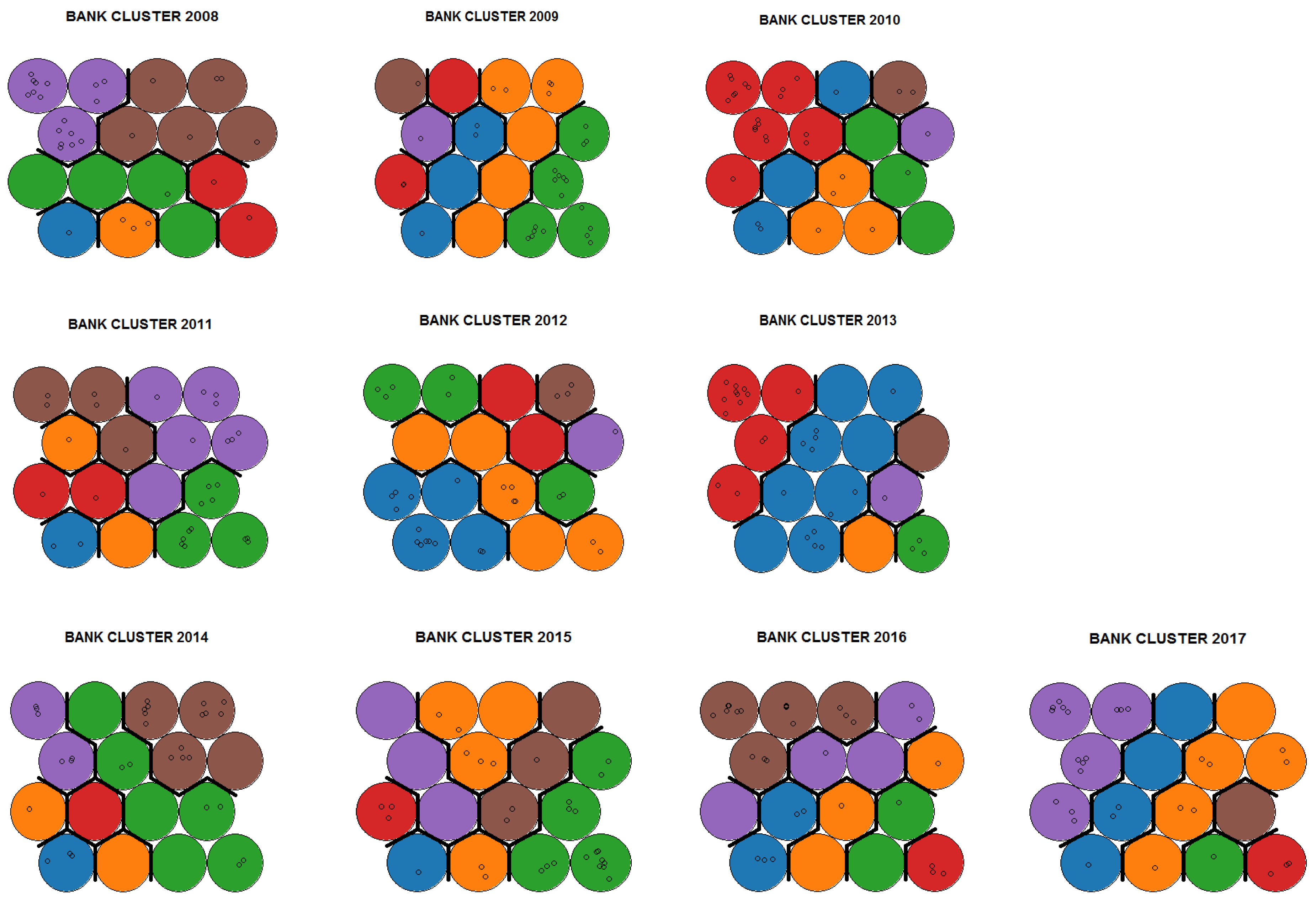
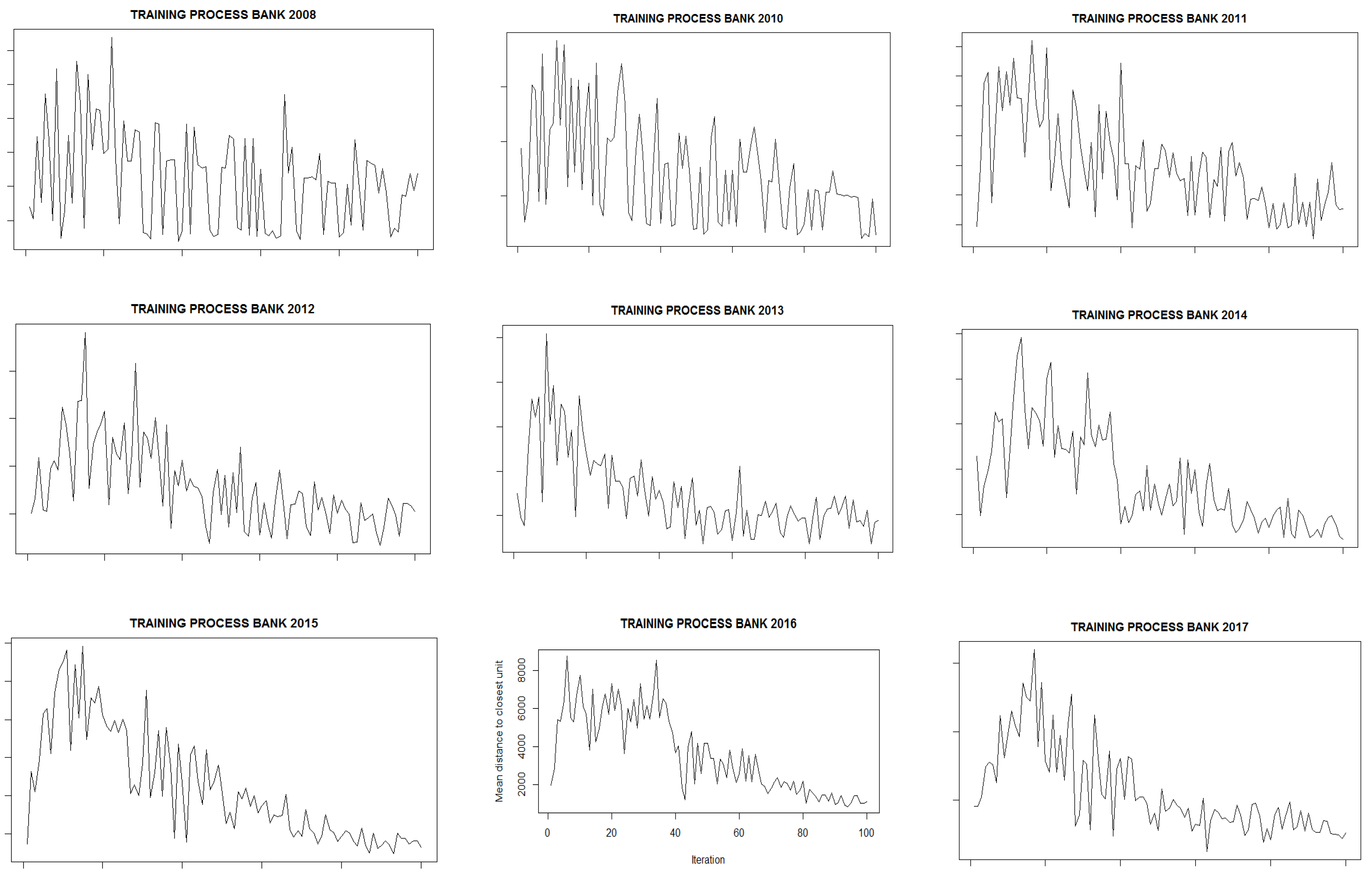
The SOM 4 × 4 grid was selected to capture the bank’s locations. The ‘hexagonal’ structure was chosen because it results in more neighbouring networks (Samarasinghe 2006). The SOM was trained repeatedly with 100 iterations and a learning rate between 0.01 to 0.02. The Euclidean distance was used to decide the winning neuron and the Gaussian neighbourhood function was used to alter weight smoothly across distance. This procedure was repeated multiple times until the SOM was thoroughly trained. The training processes (for the period of 2008 to 2017) showed that the mean distance reached a maximum and dropped to the minimum (see Appendix A Figure A1). These outcomes indicated that the 4 × 4 neuron grid was closest to the data information. As a result, the final SOM maps show the locations of Vietnam’s domestic banks in the 2D maps (see Figure 1). There were some empty neurons and some neurons that contain many banks. In short, the SOM results provide a clear picture of which banks are categorised into each specific neuron.

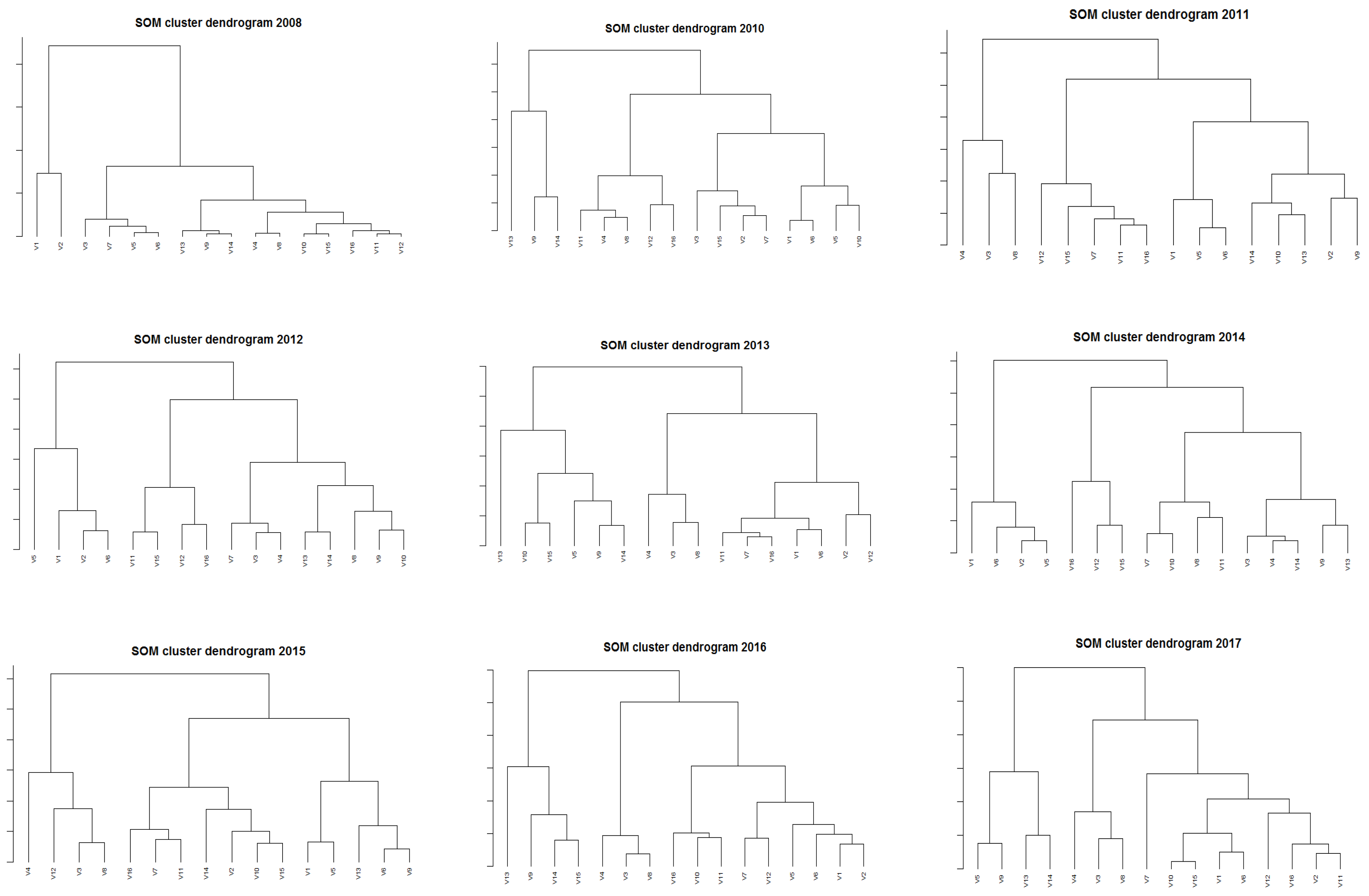
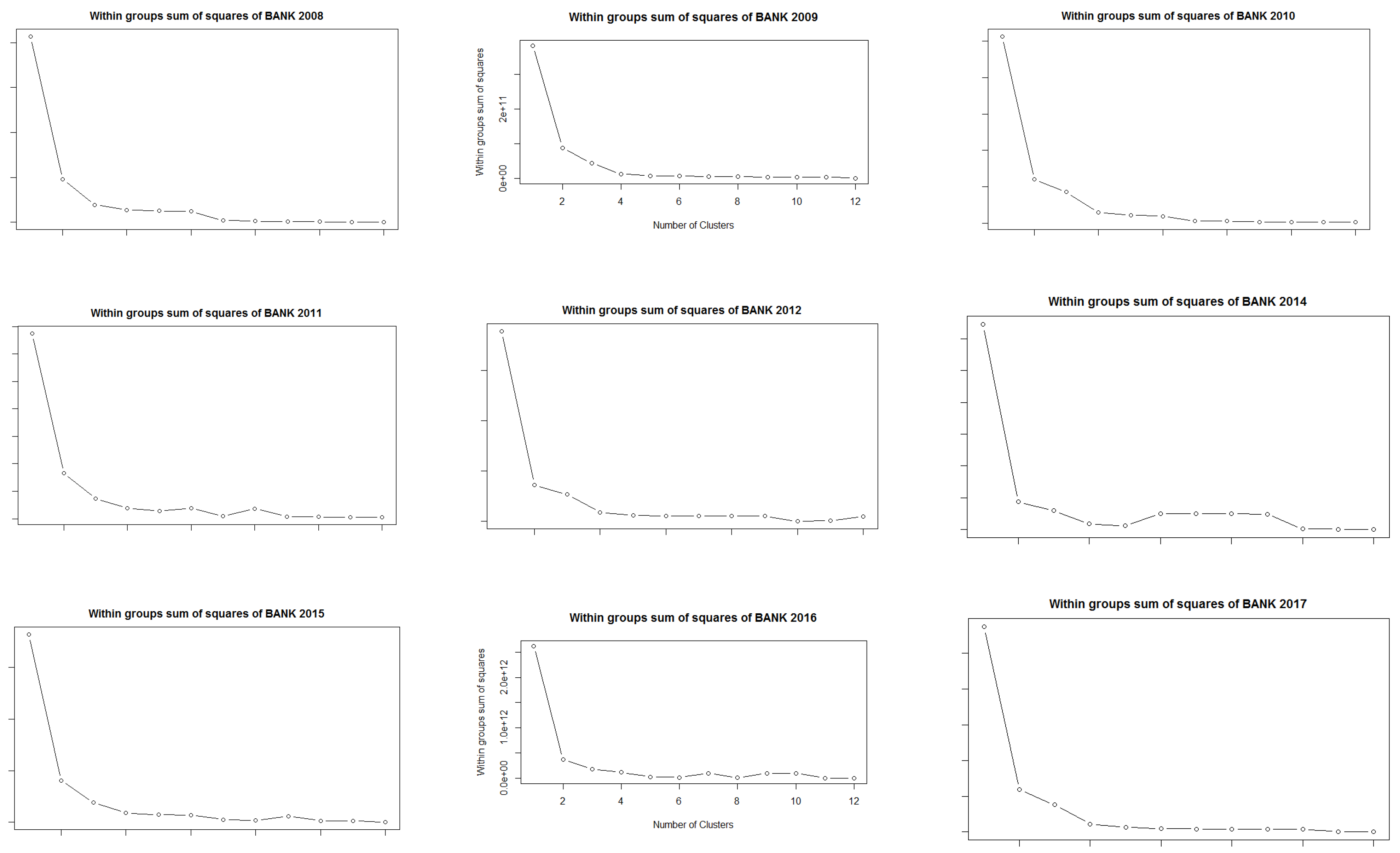
Sixteen neurons were categorised into six groups. These six groups are shown in orange, purple, red, brown, green and blue (see Figure 1). The mean within group sum of squares (WSS) was used to select the optimum number of clusters. The optimum clusters were chosen as the cluster that had the largest change in WSS value (Waidyarathne and Samarasinghe 2014). The WSS value dropped dramatically when the number of clusters increased from one to two (see Appendix A Figure A2). This suggested that the 16 neurons should be categorised into two clusters. The dendrograms also suggested that groups two to six should be grouped into one cluster (see Appendix A Figure A3). As a consequence, groups two to six were clustered to create a super-class group of banks (named group two banks). Group one is a super-class bank group (named group one). In short, super-class bank groups one and two represent two clusters of 16 neurons; in total, these represent a total of 27 banks. There were only commercial joint stock banks in group one. Group two contained four commercial state banks and several joint stock banks. The mean total assets over the 10 years was 38,053 billion VND for group one banks and 280,194 billion VND for group two banks (see Appendix A 

Table A3. Summary mean asset values for super-class group one and group two banks.

Asset Value		Unit	Value
All banks	Mean	(Billion VND)	168,001
	Standard Deviation	(Billion VND)	201,038
Group 2 banks	Mean	(Billion VND)	280,194
	Standard Deviation	(Billion VND)	220,089
Group 1 banks	Mean	(Billion VND)	38,053
	Standard Deviation	(Billion VND)	19,424

Note: this table shows mean asset values of Vietnam domestic banks (group 2 and group 1 banks). Source: author’s calculations.

). In other words, group two banks were larger (have greater total assets) than group one banks.

4.1.2. Dynamic Evaluation Phase

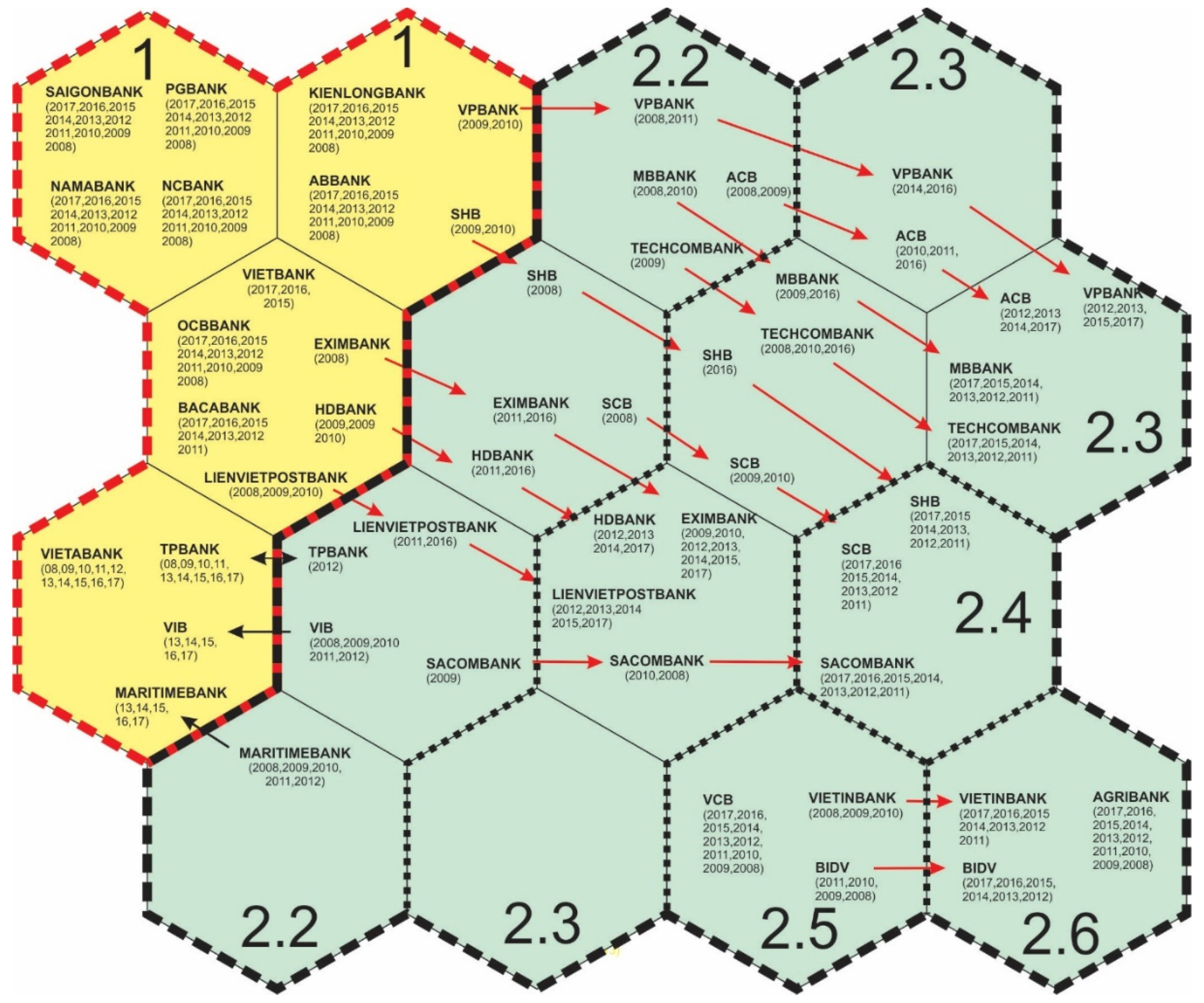
In the second step, ten 2D mapping plots (see Figure 1) for the period 2008 to 2017 were overlapped on each other. Each bank was observed and connected from neuron to neuron or group to group, to find its specific trajectory. The trajectory pattern results are shown in Figure 2.

Table 1. Bank group one and two results for the sampled banks for the period 2008 to 2017.

	2008	2009	2010	2011	2012	2013	2014	2015	2016	2017
BIDV	2	2	2	2	2	2	2	2	2	2
Agribank	2	2	2	2	2	2	2	2	2	2
Vietinbank	2	2	2	2	2	2	2	2	2	2
VCB	2	2	2	2	2	2	2	2	2	2
SCB	2	2	2	n.a	2	2	2	2	2	2
Sacombank	2	2	2	2	2	2	2	2	2	2
Mbbank	2	2	2	2	2	2	2	2	2	2
Techcombank	2	2	2	2	2	2	2	2	2	2
SHB	2	1	1	2	2	2	2	2	2	2
ACB	2	2	2	2	2	2	2	2	2	2
VPBank	2	1	1	2	2	2	2	2	2	2
HDBank	1	1	1	2	2	2	2	2	2	2
LienViet	1	1	1	2	2	2	2	2	2	2
Eximbank	1	2	2	2	2	2	2	2	2	2
TPBank	1	1	1	1	2	1	1	1	1	1
VIB	2	2	2	2	2	1	1	1	1	1
Maritimebank	2	2	2	2	2	1	1	1	1	1
BacAbank		n.a.		1	1	1	1	1	1	1
ABBank	1	1	1	1	1	1	1	1	1	1
NVB	1	1	1	1	1	1	1	1	1	1
OCB	1	1	1	1	1	1	1	1	1	1
Viet A bank	1	1	1	1	1	1	1	1	1	1
Nam A Bank	1	1	1	1	1	1	1	1	1	1
Vietbank				n.a.					1	1
KienLongBank	1	1	1	1	1	1	1	1	1	1
PGbank	1	1	1	1	1	1	1	1	1	1
Saigonbank	1	1	1	1	1	1	1	1	1	1

Note: n.a. = not available. ‘1’= group 1 banks; ‘2’ = group 2 banks. Source: author’s analysis.

shows how Vietnam domestic banks are located within super-class groups one and two for the period of 2008 to 2017. Some banks remained in the same group over the entire study period. Ten banks maintained their position in group one banks: BacAbank, ABBank, NVB, OCB, Viet A bank, Nam A Bank, Vietbank, KienLongBank, PGbank and Saigonbank. Similarly, there were nine banks in group two banks: these are BIDV, Agribank, Vietinbank, VCB, SCB, Sacombank, Mbbank, Techcombank and ACB (see Figure 2 and Table 1). However, five banks shifted positions from group one banks to group two banks: SHB, VPBank, HDBank, LienVietPostbank and Eximbank. Conversely, SHB, VPBank, HDBank. LienVietPostbank and Eximbank which were in group one banks (from 2008 to 2011) moved to group two banks (from 2012 to 2017).

4.2. Measuring Market Power for Group One and Two Banks

Our study used the non-structural Lerner index to assess the market power of Vietnam domestic banks. Appendix A 

Table A4. The financial data used to compute the Lerner index of Vietnam banks (2008–2017).

Variables			Obs	Mean	SD	Min	Max
Total Costs	TC	Billion VND	258	10,873	13,659	106	66,993
Total Assets	Q	Billion VND	258	169,857	227,337	2419	1,202,284
Total Revenue	TR	Billion VND	258	13,795	17,505	195	88,560
Price of Staff Cost	w1		258	0.0078	0.0028	0.0031	0.0184
Price of Deposits	w2		258	0.0851	0.0455	0.0316	0.3927
Price of Capital	w3		258	1.0500	1.3496	0.0792	17.3288

Note: Obs = observation; SD = standard deviation. Source: author’s computation.

lists the financial information used to quantify the Lerner index for the period of 2008 to 2017. Data were analysed using STATA software (version R15) (StataCorp 2017). The Lerner index results are displayed in

Table 2. The Lerner index values of Vietnam’s domestic banks for the period 2008 to 2017.

Year	No. of Banks	All		Group 2 Banks		Group 1 Banks
		Mean	S.D.	Mean	S.D.	Mean	S.D.
2008	25	0.185	0.167	0.226	0.153	0.140	0.176
2009	25	0.246	0.090	0.271	0.101	0.222	0.075
2010	25	0.236	0.080	0.261	0.083	0.213	0.071
2011	25	0.209	0.083	0.240	0.063	0.161	0.090
2012	26	0.173	0.089	0.196	0.081	0.130	0.092
2013	26	0.176	0.100	0.213	0.106	0.132	0.074
2014	26	0.209	0.108	0.260	0.098	0.150	0.089
2015	26	0.215	0.106	0.274	0.101	0.147	0.064
2016	27	0.216	0.118	0.274	0.118	0.154	0.085
2017	27	0.237	0.124	0.302	0.125	0.167	0.079
Mean		0.210	0.107	0.252	0.103	0.162	0.090

Note: S.D. = standard deviation. Source: author’s computation.

.

The average Lerner index score of Vietnam domestic banks for the period of 2008 to 2017 was 0.210 (see Table 2). The Lerner index score increased slightly in 2016 and 2017 (0.216 and 0.237, respectively). A slight increase in the overall Lerner index implies a decline in bank competition. This decline in bank competition could be because of the decreasing number of Vietnam domestic banks, from 43 banks in 2008 to 32 banks in 2017. Fewer banks could lead to less competition and greater bank market power. This result is similar to those found in previous studies, which have identified increased Lerner index values: Demirguc-Kunt and Martínez-Pería’s (2010) study of Jordanian banking industry and Adjei-Frimpong et al.’s (2016) study of the Ghanaian banking industry.

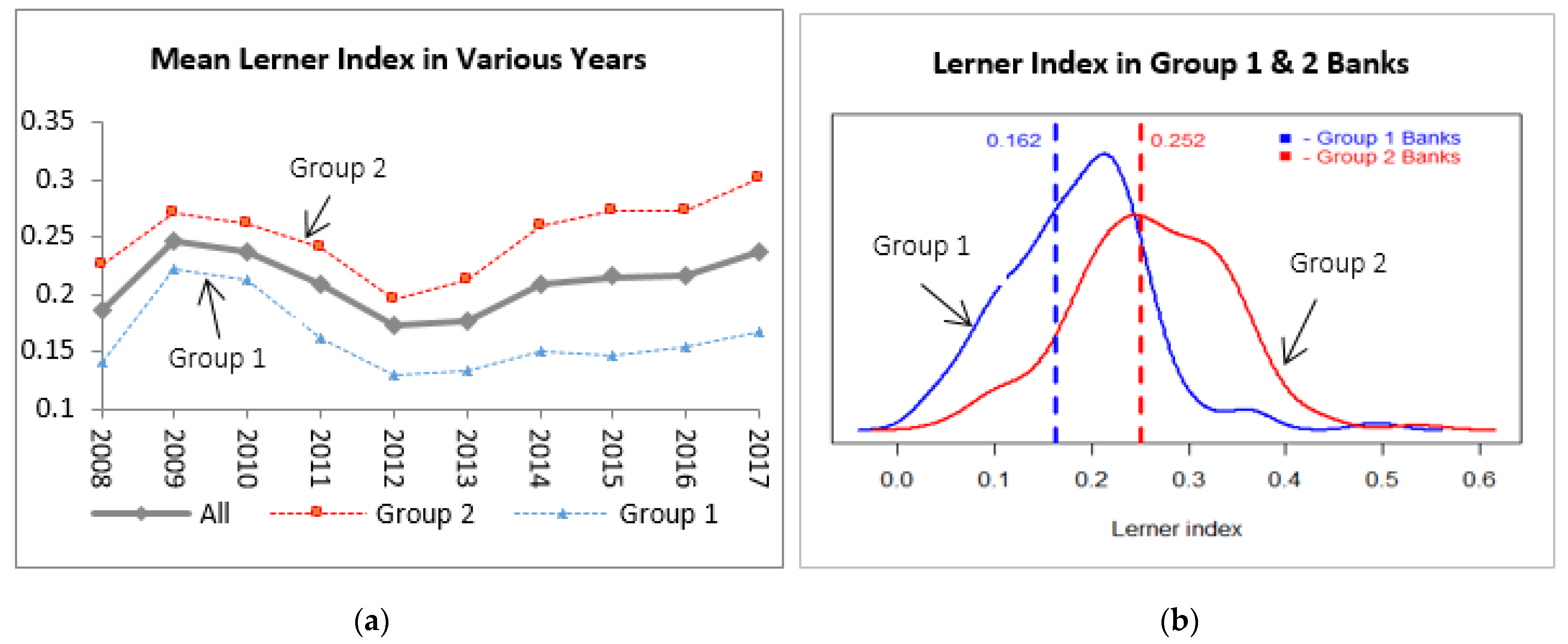
Figure 3 shows the Lerner index scores for both group one and two banks for the period of 2008 to 2017. The average Lerner score of group one banks was higher than both the average group two banks’ Lerner scores and the average for all banks for the period from 2008 to 2017 (see Figure 3a). The average Lerner index for group two banks was 0.252, which was higher than group one banks (0.162) by approximately 56% (see Figure 3b). This outcome implies that group two banks are stronger (or have greater market power) than group one banks. The paired t-test was used to examine the statistical significance of the difference in the Lerner indexes between group one and two banks. The null hypothesis ($H_0$) is that the mean difference in the Lerner indexes between groups one and two banks is zero. The t-test results were statistically significant at the 1% level (t-value equals −6.83). This result indicates a rejection of the null hypothesis. In other words, there was a statistically significant difference in bank market power between group one and two banks.

Our result contradicts Nguyen and Nghiem’s (2018) study, which showed that the difference in market power between commercial state and joint stock banks was not statistically significant. The contradictory results imply that the grouping approach that categorises state and joint stock Vietnam banks may be inappropriate when testing differences in market power between these banks. In contrast, the SOM technique, which uses an unsupervised algorithm, can better capture differences in bank market power and categorise Vietnam domestic banks into two super-class groups: group one and two. Group twp banks (with a mean of Lerner index value of 0.252) have greater market power than group one banks (with a value of 0.162). Group two banks also have greater total assets than group one banks (see Appendix A Table A3).

4.3. Measuring the Efficiency of Group One and Two Banks

The non-parametric DEA technique under the VRS assumption was used to compute bank performance (represented by CE scores). Appendix A 

Table A5. Summary statistics of the financial data used to compute Vietnam bank efficiency (2008–2017).

Variable			Obs	Mean	SD	Min	Max
Total Deposits	x1	Billion VND	258	128,325	189,744	1172	1,011,314
Labour (Staff Costs)	x2	Billion VND	258	1424	2112	20	11,195
Fixed Assets	x3	Billion VND	258	1823	2272	46	11,437
Loans	y1	Billion VND	258	105,912	165,211	275	863,575
Other Earning Assets	y2	Billion VND	258	51,451	61,186	542	462,597
Price of staff cost	w1		258	0.0078	0.0028	0.0031	0.0184
Price of Deposits	w2		258	0.0851	0.0455	0.0316	0.3927
Price of Capital	w3		258	1.0500	1.3496	0.0792	17.3288

Note: Obs = observation; SD = standard deviation. Source: author’s computation.

provides the statistical data used to compute CE scores for the period of 2008 to 2017. The dataset was estimated using the R program (version 3.4.2) with the “Benchmarking” package (R Core Team 2017). Bogetoft and Otto’s (2018) “Benchmarking” software package was employed to estimate CE scores using the DEA method.

Table 3. CE scores for Vietnam banks (for the period 2008–2017).

Year	No. of Banks	All Banks		Group 2		Group 1
		Mean	S.D.	Mean	S.D.	Mean	S.D.
2008	25	0.872	0.133	0.885	0.138	0.858	0.133
2009	25	0.923	0.083	0.934	0.087	0.913	0.082
2010	25	0.940	0.098	0.944	0.097	0.937	0.104
2011	25	0.732	0.253	0.786	0.254	0.675	0.249
2012	26	0.888	0.147	0.909	0.160	0.849	0.117
2013	26	0.838	0.143	0.847	0.147	0.827	0.145
2014	26	0.856	0.140	0.872	0.127	0.838	0.158
2015	26	0.882	0.130	0.866	0.134	0.901	0.127
2016	27	0.795	0.154	0.772	0.165	0.819	0.142
2017	27	0.824	0.160	0.770	0.176	0.882	0.123
Mean		0.855	0.144	0.858	0.148	0.850	0.138

Note: S.D. = standard deviation. Source: author’s computation.

shows the CE scores of the banks. The mean CE score was 0.855, which indicates that Vietnam domestic banks could reduce their costs by 14.5% (from 100% to 85.5%), while maintaining the same outputs.

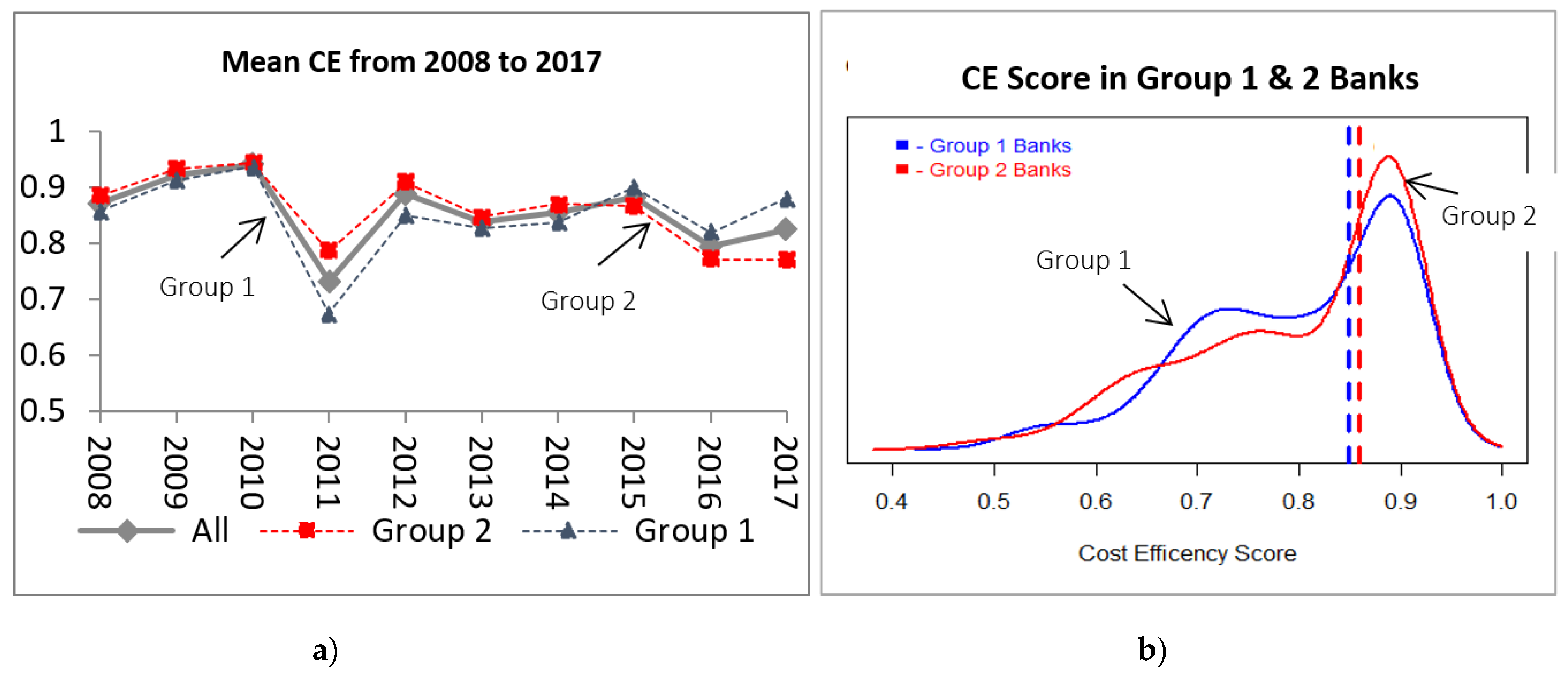
Figure 4 show the CE scores for the two groups of banks. The mean CE scores for both groups of banks were quite similar (see Figure 4a). The average CE score for group two banks was 0.858: this is 1% higher than the average CE score of group one banks (0.850) (see Figure 4b). The paired t-test was used to test the difference between the CE scores for the two groups of banks. The null hypothesis (H0) was that the difference of CE scores between group one and two banks would equal zero. The t-value was insignificant at all conventional levels. The p-values of the paired CE tests was 0.5817. These results confirm the null hypothesis. In short, the differences in CE scores for groups one and two banks were insignificant. These findings echo previous studies (Nguyen and Nghiem 2018; Vu and Turnell 2010). The authors found no significant differences between the CE scores of commercial state-owned and joint stock banks in Vietnam.

5. Conclusions and Policy Implications

This study used the SOM technique to categorise Vietnam domestic banks into two super-class groups (one and two). While differences in the Lerner scores (which represent market power) between the two super-class bank groups (one and two) were statistically significant at the 1% level, the CE scores (which represent performance) were the same. The different market power between group one and two banks contradict Nguyen and Nghiem’s (2018) results. This study shows that the SOM technique (with an unsupervised algorithm) can better capture differences in bank market power and thus can be used to divide Vietnam domestic banks into two groups, consisting of weak banks (group one) and strong banks (group two). Using the SOM technique provides academics with a new approach, which is based on an unsupervised algorithm. This is different from previous studies, which have divided domestic Vietnam banks into commercial state and joint stock banks (Nguyen and Nghiem 2018; Vu and Turnell 2010). Hence, this study has argued that two groups of banks with different levels of market power exist side-by-side in the Vietnam banking industry. The group of strong banks tends to be monopolists. The existence of these two groups of banks (weak and strong banks) indicates that the competitive domestic banking environment in Vietnam may be at risk. The reason is that group two banks may be more profitable due to greater market power, whereas group one banks may struggle to cut costs to remain viable.

Group two banks (the larger banks) occupy the dominant position in this environment and will continue to expand (Tabak et al. 2012; Wang 2015). In such an environment, group two banks may end up acquiring group one banks. This explains why the number of banks reduced from 43 to 32 over the study period of 2008 to 2017. Policymakers and regulators must take this phenomenon (group two banks acquiring group one banks) into consideration when issuing policies in order to maintain an optimal number of banks to ensure the stability and competitiveness of the Vietnam banking system. As Le (2014) notes, the ideal number of banks to achieve stability in the Vietnam banking system is between 15 and 17. In 2017, there were 32 banks. To meet the ideal number, half would need to be merged.

Our SOM results showed that 70% of Vietnam banks (19 of 27 banks) maintained their positions, either in super-class group one or two banks. This result indicates that banks tend to maintain their financial position in the industry, and that bank market power persists over time. This fact indicates the existence of some rigidity in the banking industry, which may make it difficult for weak banks to compete. Future research could consider whether bank market power persists over a long period of time. These findings will help policymakers and regulators avoid rigidity and ensure an efficient and competitive banking environment.

References

1. Abel, Sanderson, and Pierre le Roux. 2017. Evaluating Market Power in the Zimbabwean Banking Sector. Journal of Economic and Financial Sciences 10: 274–91. [Google Scholar] [CrossRef] [Green Version]
2. Ab-Rahim, Rossazana. 2017. Efficiency and Competition in the Malaysian Banking Market: Foreign versus Domestic Banks. Gadjah Mada International Journal of Business 19: 193–221. [Google Scholar] [CrossRef] [Green Version]
3. Adjei-Frimpong, Kofi, Christopher Gan, and Baiding Hu. 2014. Cost efficiency of Ghana’s banking industry: A panel data analysis. The International Journal of Business and Finance Research 8: 69–86. [Google Scholar]
4. Adjei-Frimpong, Kofi, Christopher Gan, and Baiding Hu. 2016. Competition in the banking industry: Empirical evidence from Ghana. Journal of Banking Regulation 17: 159–75. [Google Scholar] [CrossRef]
5. Angelini, Paolo, and Nicola Cetorelli. 2003. The Effects of Regulatory Reform on Competition in the Banking Industry. Journal of Money, Credit, and Banking 35: 663–84. [Google Scholar] [CrossRef]
6. Barth, James R., Chen Lin, Yue Ma, Jesús Seade, and Frank M. Song. 2013. Do bank regulation, supervision and monitoring enhance or impede bank efficiency. Journal of Banking & Finance 37: 2879–92. [Google Scholar]
7. Bogetoft, Peter, and Lars Otto. 2018. Benchmarking with DEA and SFA, R Package Version 0.27. Berlin: Springer Science & Business Media. [Google Scholar]
8. Chen, Mu-Yen. 2012. Visualization and dynamic evaluation model of corporate financial structure with self-organizing map and support vector regression. Applied Soft Computing 12: 2274–88. [Google Scholar] [CrossRef]
9. Chen, Ning, Bernardete Ribeiro, Armando Vieira, and An Chen. 2013. Clustering and visualization of bankruptcy trajectory using self-organizing map. Expert Systems with Applications 40: 385–93. [Google Scholar] [CrossRef]
10. Delis, Manthos D., and George Pagoulatos. 2009. Bank Competition, Institutional Strength and Financial Reforms in Central and Eastern Europe and the EU. MPRA Paper 16494. Munich: University Library of Munich. [Google Scholar]
11. Demirguc-Kunt, Asli, and María Soledad Martínez-Pería. 2010. A Framework for Analyzing Competition in the Banking Sector: An Application to the Case of Jordan. Policy Research Working Paper Series 5499; Washington, DC: The World Bank. [Google Scholar]
12. Du Jardin, Philippe, and Eric Séverin. 2011. Predicting corporate bankruptcy using a self-organizing map: An empirical study to improve the forecasting horizon of a financial failure model. Decision Support Systems 51: 701–11. [Google Scholar] [CrossRef] [Green Version]
13. Du Jardin, Philippe, and Eric Séverin. 2012. Forecasting financial failure using a Kohonen map: A comparative study to improve model stability over time. European Journal of Operational Research 221: 378–96. [Google Scholar] [CrossRef] [Green Version]
14. Fernández de Guevara, Juan, Joaquín Maudos, and Francisco Pérez. 2005. Market Power in European Banking Sectors. Journal of Financial Services Research 27: 109–37. [Google Scholar] [CrossRef]
15. Gardener, Edward, Philip Molyneux, and Hoai Nguyen-Linh. 2011. Determinants of efficiency in South East Asian banking. The Service Industries Journal 31: 2693–719. [Google Scholar] [CrossRef]
16. Hoang, Hoang Thi Thanh, Phan Dien Vy, and Jay Bandaralage. 2016. Mergers, Acquisitions and Market Concentration in the Banking Sector: The Case of Vietnam. Asian Journal of Economics and Empirical Research 3: 49–58. [Google Scholar] [CrossRef] [Green Version]
17. Kočišová, Kristína. 2014. Application of Data Envelopment Analysis to Measure Cost, Revenue and Profit Efficiency. Statistika: Statistics and Economy Journal 94: 47–57. [Google Scholar]
18. Kohonen, Teuvo. 1982. Self-organized formation of topologically correct feature maps. Biological Cybernetics 43: 59–69. [Google Scholar] [CrossRef]
19. KPMG. 2013. Vietnam Banking Survey. Amstelveen: KPMG Limited. [Google Scholar]
20. Le, Trung H. 2014. Market Concentration and Competition in Vietnamese Banking Sector. MPRA Paper 57406. Germany: University Library of Munich. Available online: https://ideas.repec.org/p/pra/mprapa/57406.html (accessed on 1 July 2018).
21. Liu, Hong, Philip Molyneux, and Linh H. Nguyen. 2012. Competition and risk in South East Asian commercial banking. Applied Economics 44: 3627–44. [Google Scholar] [CrossRef] [Green Version]
22. Nadeem, Muhammad, Christopher Gan, and Cuong Nguyen. 2017. Does intellectual capital efficiency improve firm performance in BRICS economies? A dynamic panel estimation. Measuring Business Excellence 21: 65–85. [Google Scholar] [CrossRef]
23. Nguyen, Hoang Phong. 2018. Profitability of Vietnamese Banks Under Competitive Pressure. Emerging Markets Finance and Trade 55: 2004–21. [Google Scholar] [CrossRef]
24. Nguyen, Thanh Pham Thien, and Son Hong Nghiem. 2018. The effects of competition on efficiency: The Vietnamese banking industry experience. The Singapore Economic Review 63: 1–30. [Google Scholar] [CrossRef]
25. Nguyen, Thanh Pham Thien, Eduardo Roca, and Parmendra Sharma. 2014. How efficient is the banking system of Asia’s next economic dragon? Evidence from rolling DEA windows. Applied Economics 46: 2665–84. [Google Scholar] [CrossRef]
26. Nguyen, Thanh Pham Thien, Son Hong Nghiem, Eduardo Roca, and Parmendra Sharma. 2016a. Bank reforms and efficiency in Vietnamese banks: Evidence based on SFA and DEA. Applied Economics 48: 2822–35. [Google Scholar] [CrossRef] [Green Version]
27. Nguyen, Thanh Pham Thien, Son Hong Nghiem, Eduardo Roca, and Parmendra Sharma. 2016b. Efficiency, innovation and competition: Evidence from Vietnam, China and India. Empirical Economics 51: 1235–59. [Google Scholar] [CrossRef]
28. R Core Team. 2017. A Language and Environment for Statistical Computing, 4.3.2 ed. Vienna: R Foundation for Statistical Computing. [Google Scholar]
29. Samarasinghe, Sandhya. 2006. Neural Networks for Applied Sciences and Engineering. Boston: Auerbach Publications. [Google Scholar]
30. StataCorp. 2017. Stata Statistical Software: Release 15. College Station: StataCorp LLC. [Google Scholar]
31. The State Bank of Vietnam. 2018. Available online: https://www.sbv.gov.vn/webcenter/portal/en/ (accessed on 1 July 2018).
32. Tabak, Benjamin M., Dimas M. Fazio, and Daniel O. Cajueiro. 2012. The relationship between banking market competition and risk-taking: Do size and capitalization matter? Journal of Banking & Finance 36: 3366–81. [Google Scholar]
33. Tsai, Chih-Fong, and Ming-Lun Chen. 2010. Credit rating by hybrid machine learning techniques. Applied Soft Computing 10: 374–80. [Google Scholar] [CrossRef]
34. Vu, Ha Thu, and Sean Turnell. 2010. Cost Efficiency of the Banking Sector in Vietnam: A Bayesian Stochastic Frontier Approach with Regularity Constraints. Asian Economic Journal 24: 115–39. [Google Scholar] [CrossRef]
35. Waidyarathne, K. Pramuditha, and Sandhya Samarasinghe. 2014. Artificial neural networks to identify naturally existing disease severity status. Neural Computing and Applications 25: 1031–41. [Google Scholar] [CrossRef]
36. Wang, Tianxi. 2015. Competition and Increasing Returns to Scale: A Model of Bank Size. The Economic Journal 125: 989–1014. [Google Scholar] [CrossRef] [Green Version]
37. Wehrens, Ron, and Lutgarde M. C. Buydens. 2007. Self- and Super-organizing Maps in R: The kohonen Package. Journal of Statistical Software 21: 1–19. [Google Scholar] [CrossRef] [Green Version]
Figure 1. The 2D SOM map results separating Vietnam banks into categories at each specific neuron and group for the period 2008 to 2017. Note: orange, purple, red, brown, green and blue indicate groups 1 to 6. Source: author’s computation.
Jrfm 14 00485 g001
Figure 2. Final trajectory patterns of Vietnam banks for the period 2008 to 2017. Note: ‘1’ = super-class group 1 bank; ‘2’ = super-class group 2 bank; 2.2 to 2.6 = groups 2 to 6 are classified as super-class group 2 banks. Source: author’s computation.
Jrfm 14 00485 g002
Figure 3. The average Lerner index for group 1 and group 2 Vietnam banks for the period 2008 to 2017. Source: author’s computation.
Jrfm 14 00485 g003
Figure 4. The mean CE scores of Vietnam’s group 1 and 2 banks for the period 2008 to 2017. Notes: CE = cost-efficiency. Source: author’s computation.
Jrfm 14 00485 g004