
Make the Best from Comparing Conventional and Islamic Asset Classes: A Design of an All-Seasons Combined Portfolio


Abstract
:“The COVID-19 is not a Black Swan. It was more predictable than people realise.The Black Swan was meant to explain why, in a networked world, we need to change business practices and social norms not to provide a cliché for any bad thing that surprises us.”Nassim Taleb
1. Introduction
- The renewed attention to assets uncorrelated or negatively correlated with other traditional assets, such as gold, precious metals, commodities, or treasuries, providing portfolio-diversification benefits in terms of volatility, downside risk, and maximum drawdown mitigation power, particularly during financial downturns (Baur and Lucey 2010; Baur and McDermott 2010; Bouri et al. 2020; Ji et al. 2020; Kristoufek 2020; Reboredo 2013).
- The hedging benefits and resilience of Islamic equities during the last great GFC are attributed to the limited exposure to high-leverage companies due to the Shariah screening (Ashraf et al. 2020; Jawadi et al. 2014). IFS distinguishes itself by promoting a more ethical approach to profit and risk sharing, facilitating fairness in financial matters (Al Rahahleh et al. 2019).
- The academic interest in the Islamic Stock Market (ISM) compared to the conventional one has divergent results in terms of performance (Belouafi et al. 2015; Delle Foglie and Panetta 2020; Hassan et al. 2019; Masih et al. 2018). Delle Foglie and Panetta (2020) proposed a change in the research approach, searching for the possibility to evaluate the Shariah-compliant instrument diversification, decoupling and hedging benefits, and combining the conventional portfolio and not merely different asset classes.
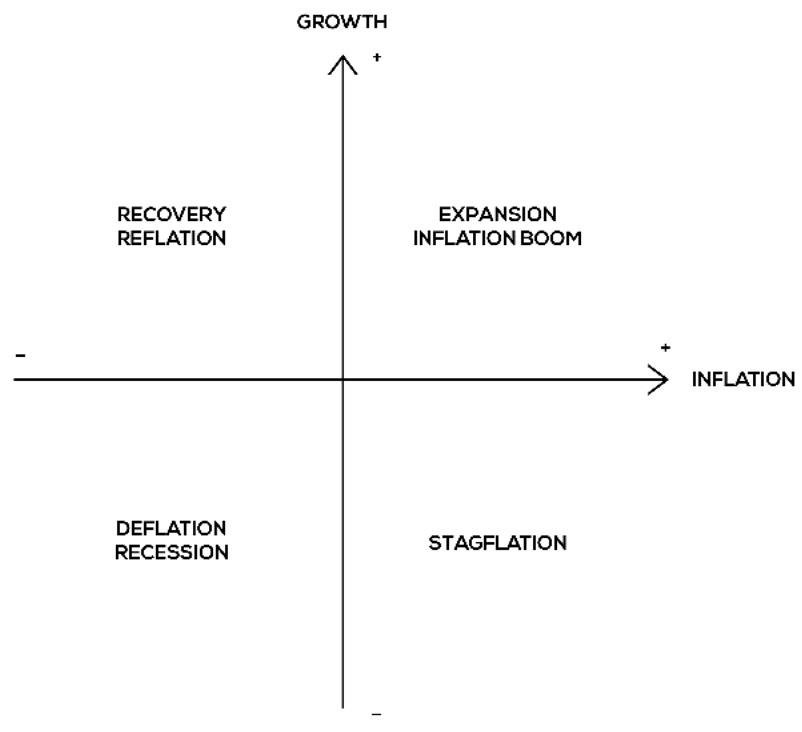
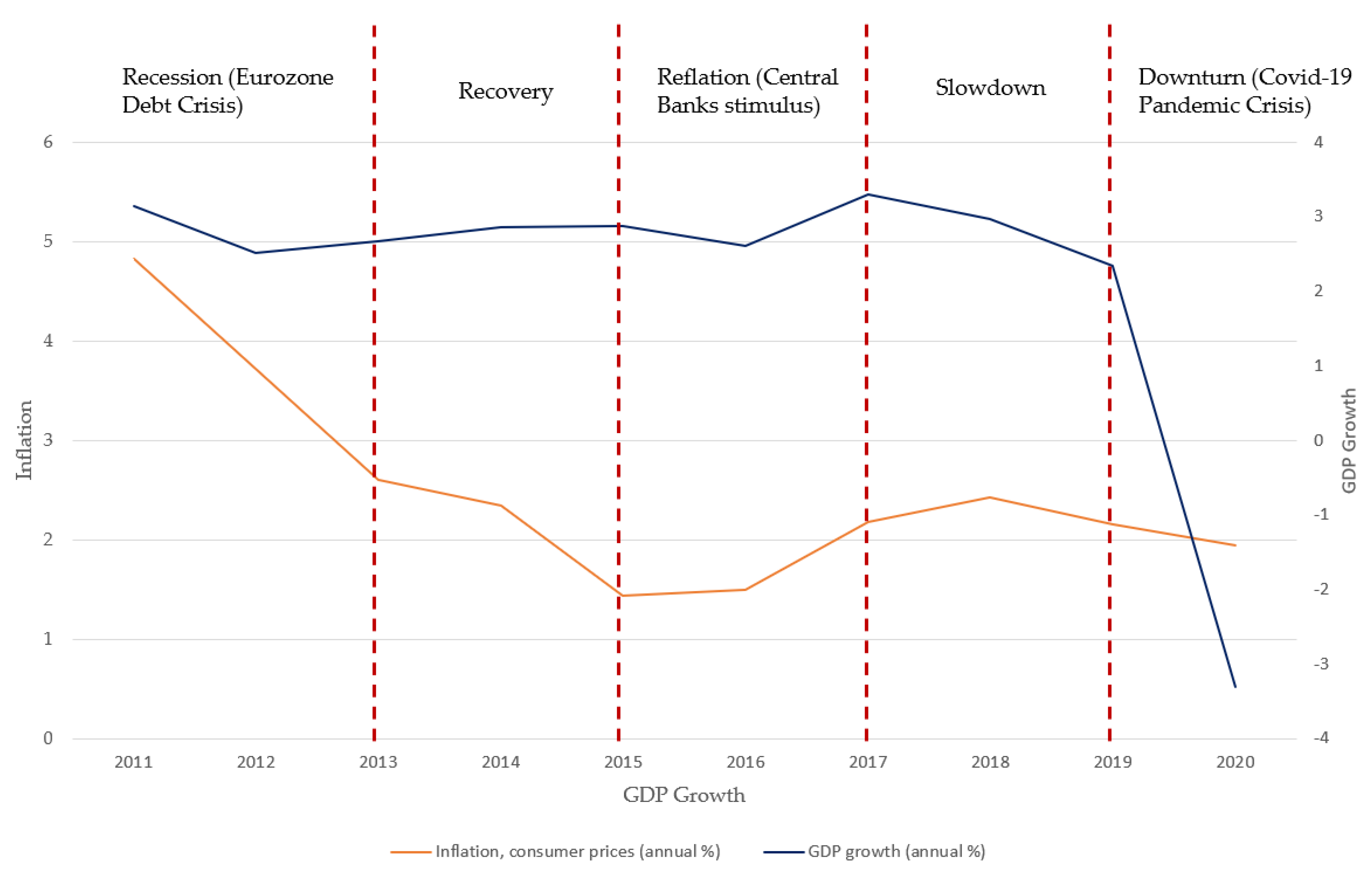
- The financial crisis increases the need to design a portfolio strategy that fits all macroeconomic environments, and faces the current postcrash scenario and future economic and financial uncertainty. Assuming every economic cycle is a set of unpredictable chronological events affecting each specific asset class performance, it seems unnecessary to forecast the next financial downturns, since it is impossible to predict the future (Economic machine—Bridgewater 2011). This principle also corresponds to the theoretical background underlying the foundation of Global Macro Anima (GMA), a strategic asset allocation based on the diversification across macroeconomic scenarios proposed by Pola (2013, 2021). The GMA approach overcomes the mean-variance framework that dominates portfolio strategies, declaring that “asset–return dynamics can be explained mainly by variations of expectations rather than the levels of macroeconomic variables”.
2. Methodology
2.1. The All-Weather Philosophy and the GMA Strategy
2.2. The Risk Parity Model and the Optimisation Problem
- -
- b and beq are vectors, A and Aeq are matrices, c(x) and ceq(x) are functions that return vectors, and f(x) is a function that returns a scalar. f(x), c(x), and ceq(x) can be nonlinear functions.
- -
- x, lb, and ub can be passed as vectors or matrices.
- Internally, solvers convert matrix arguments into vectors before processing. For example, x0 becomes x0(:);
- For output, solvers reshape the solution, x, to the same size as the input, x0;
- When x0 is a matrix, solvers pass x as a matrix of the same size as x0 to both the objective function and to any nonlinear constraint function;
- Linear constraints, however, take x in vector form, x(:). In other words, a linear constraint of the form:
((EW_Shares’) * VarCovar (:,:,1) * EW_Shares))). * EW_Shares − (sqrt
((EW_Shares’) * VarCovar (:,:,1) * EW_Shares))/nc).^2}
2.3. Data and Sample Selection
3. Empirical Results
3.1. Descriptive Statistics and Correlation
3.2. Conventional Portfolio ERC Optimisation
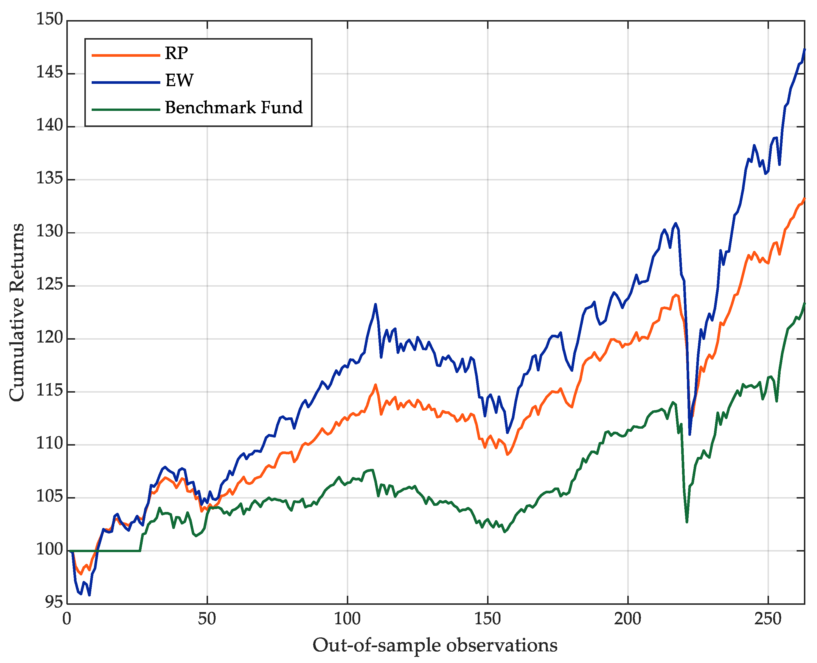
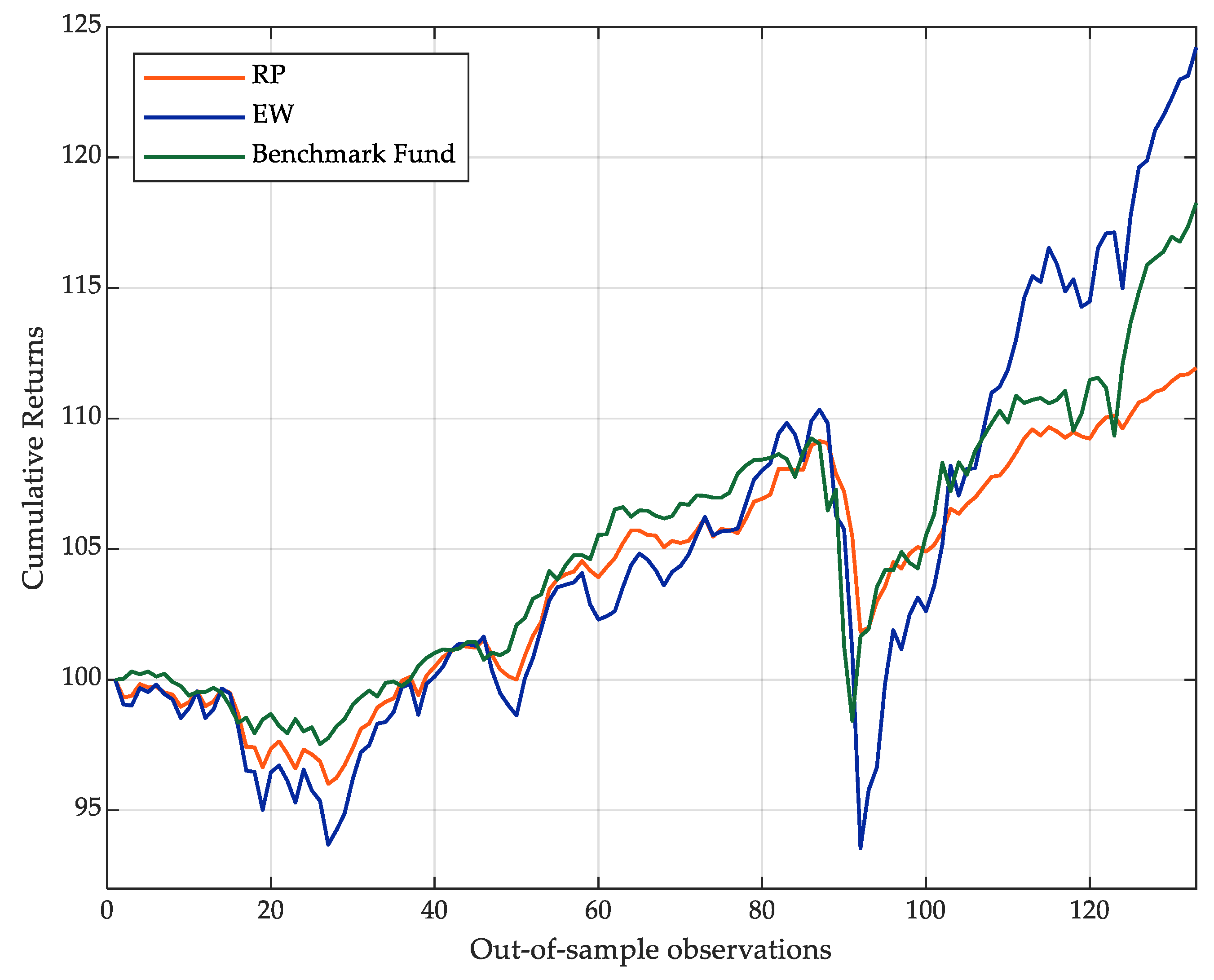
3.3. Combined Portfolio ERC Optimisation
4. Conclusions and Further Research
Author Contributions
Funding
Institutional Review Board Statement
Informed Consent Statement
Data Availability Statement
Acknowledgments
Conflicts of Interest
References
- Al Rahahleh, Naseem, M. Ishaq Bhatti, and Faridah Najuna Misman. 2019. Developments in Risk Management in Islamic Finance: A Review. Journal Risk Financial Manag 12: 37. [Google Scholar] [CrossRef] [Green Version]
- Allen, Gregory. 2010. The Risk Parity Approach to Asset Allocation. Shankill: Callan Investments Institute, Callan Associates. [Google Scholar]
- Anderson, Robert M., Stephen W. Bianchi, and Lisa R. Goldberg. 2012. Will My Risk Parity Strategy Outperform? Financial Analysts Journal 68: 75–93. [Google Scholar] [CrossRef] [Green Version]
- Arouri, Mohamed El Hedi, Hachmi Ben Ameur, Nabila Jawadi, Fredj Jawadi, and Waël Louhichi. 2013. Are Islamic finance innovations enough for investors to escape from a financial downturn? Further evidence from portfolio simulations. Applied Economics 45: 3412–20. [Google Scholar] [CrossRef]
- Ashraf, Dawood, Muhammad Suhail Rizwan, and Ghufran Ahmad. 2020. Islamic Equity Investments and the COVID-19 Pandemic. Available online: https://ssrn.com/abstract=3611898. (accessed on 10 February 2021).
- Baur, Dirk, and Brian Lucey. 2010. Is Gold a Hedge or a Safe Haven? An Analysis of Stocks, Bonds and Gold. The Financial Review 45: 217–29. [Google Scholar] [CrossRef]
- Baur, Dirk, and Thomas McDermott. 2010. Is gold a safe haven? International evidence. Journal of Banking & Finance 34: 1886–98. [Google Scholar]
- Belouafi, Ahmed, Chaouki Achour Bourakba, and Karima Saci. 2015. Islamic Finance and Financial Stability: A Review of the Literature. Journal of King Abdulaziz University: Islamic Economics. 28. Available online: https://ssrn.com/abstract=3063842. (accessed on 10 February 2021).
- Borio, Claudio. 2020. The COVID-19 economic crisis: Dangerously unique. Business Economics 55: 181–90. [Google Scholar] [CrossRef]
- Bouri, Elie, Rangan Gupta, and Xuan Vinh Vo. 2020. Jumps in Geopolitical Risk and the Cryptocurrency Market: The Singularity of Bitcoin. Defence and Peace Economics. [Google Scholar] [CrossRef]
- Bridgewater, L. P. 2011. The All Weather Story. Available online: https://www.bridgewater.com/research-and-insights/the-all-weather-story (accessed on 10 February 2021).
- Bridgewater, L. P. 2012. Risk Parity Is about Balance. Available online: https://www.bridgewater.com/research-and-insights/risk-parity-is-about-balance (accessed on 10 February 2021).
- Bruder, Benjamin, and Thierry Roncalli. 2012. Managing Risk Exposures Using the Risk Budgeting Approach. Available online: https://ssrn.com/abstract=2009778 (accessed on 10 February 2021).
- Byrd, Richard H., Jean Charles Gilbert, and Jorge Nocedal. 2000. A trust region method based on interior point techniques for nonlinear programming. Mathematical Programming 89: 149–85. [Google Scholar] [CrossRef] [Green Version]
- Choueifaty, Yves, and Yves Coignard. 2008. Toward Maximum Diversification. The Journal of Portfolio Management 35: 40–51. [Google Scholar] [CrossRef] [Green Version]
- Delle Foglie, Andrea, and Ida Claudia Panetta. 2020. Islamic stock market versus conventional: Are islamic investing a ‘Safe Haven’ for investors? A systematic literature review. Pacific-Basin Finance Journal 64: 101435. [Google Scholar] [CrossRef]
- Foresti, Steven J., and Michael E. Rush. 2010. Risk-Focused Diversification: Utilising Leverage within Asset Allocation. California: Wilshire Consulting. [Google Scholar]
- Giuzio, Margherita. 2017. Genetic algorithm versus classical methods in sparse index tracking. Decisions in Economics and Finance 40: 243–56. [Google Scholar] [CrossRef]
- Haroon, Omair, Mohsin Ali, Abdullah Khan, Mudeer A. Khattak, and Syed Aun R. Rizvi. 2021. Financial Market Risks during the COVID-19 Pandemic. Emerging Markets Finance and Trade 57: 2407–14. [Google Scholar] [CrossRef]
- Hasan, Md Bokhtiar, Masnun Mahi, M. Kabir Hassan, and Abul Bashar Bhuiyan. 2021. Impact of COVID-19 pandemic on stock markets: Conventional vs. Islamic indices using wavelet-based multi-timescales analysis. The North American Journal of Economics and Finance 58: 101504. [Google Scholar] [CrossRef]
- Hassan, M. Kabir, Sirajo Aliyu, Andrea Paltrinieri, and Ashraf Khan. 2019. A Review of Islamic Investment Literature. Economic Pappers 38: 345–80. [Google Scholar] [CrossRef]
- Jawadi, Fredj, Nabila Jawadi, and Wael Louhichi. 2014. Conventional and Islamic stock price performance: An empirical investigation. International Economics 137: 73–87. [Google Scholar] [CrossRef]
- Ji, Qiang, Dayong Zhang, and Yuqian Zhao. 2020. Searching for safe-haven assets during the COVID-19 pandemic. International Review of Financial Analysis 71: 101526. [Google Scholar] [CrossRef]
- Kristoufek, Ladislav. 2020. Grandpa, grandpa, tell me the one about Bitcoin being a safe haven: Evidence from the COVID-19 pandemics. arXiv arXiv:2004.00047. [Google Scholar]
- Lee, Wai. 2011. Risk-Based Asset Allocation: A New Answer to an Old Question? Journal of Portfolio Management 37: 11–28. [Google Scholar] [CrossRef]
- Levell, Christopher. 2010. Risk Parity: In the Spotlight after 50 Years. Zagreb: General Research, NEPC. [Google Scholar]
- Lohre, Harald, Ulrich Neugebauer, and Carsten Zimmer. 2012. Diversified Risk Parity Strategies for Equity Portfolio Selection. Journal of Investing 21: 111–28. Available online: https://ssrn.com/abstract=2049280 (accessed on 10 February 2021). [CrossRef]
- Maillard, Sébastien, Thierry Roncalli, and Jérôme Teïletche. 2010. The properties of equally weighted risk contribution portfolios. The Journal of Portfolio Management 36: 60–70. [Google Scholar] [CrossRef]
- Mansor, Fadillah, M. Ishaq Bhatti, Shafiqur Rahman, and Hung Quang Do. 2020. The Investment Performance of Ethical Equity Funds in Malaysia. Journal of Risk and Financial Management 13: 219. [Google Scholar] [CrossRef]
- Masih, Mansur, Nazrol K. M. Kamil, and Obiyathulla I. Bacha. 2018. Issues in Islamic Equities: A Literature Survey. Emerging Markets Finance and Trade 54: 1–26. [Google Scholar] [CrossRef]
- MathWorks Inc. 2021. Linear Programming Solver. Available online: https://it.mathworks.com/help/optim/ug/linprog.html (accessed on 25 May 2021).
- Meucci, Attilio. 2007. Risk Contributions from Generic User-defined Factors. The Risk Magazine, 84–88. Available online: https://ssrn.com/abstract=930034 (accessed on 25 January 2021).
- Meucci, Attilio. 2009. Managing Diversification. Risk 22: 74–79. [Google Scholar]
- Mussafi, Noor Saif Muhammad, and Zuhaimy Ismail. 2021. Optimum Risk-Adjusted Islamic Stock Portfolio Using the Quadratic Programming Model: An Empirical Study in Indonesia. Journal of Asian Finance, Economics and Business 8: 839–50. [Google Scholar] [CrossRef]
- Paltrinieri, Andrea, Mohammad Kabir Hassan, Salman Bahoo, and Ashraf Khan. 2019. A bibliometric review of sukuk literature. International Review of Economics & Finance. [Google Scholar] [CrossRef]
- Pola, Gianni. 2013. Managing Uncertainty with Dams. Assets’ Segmentation in Response to Macroeconomic Changes. AMUNDI Working-Paper 2013. AMUNDI Investment Strategy Collected Research Papers 2014. Paris: AMUNDI. [Google Scholar]
- Pola, Gianni. 2021. Untangling Complexity in Financial Markets. A New Paradigm for Asset Allocation. ANIMA Working Paper Series, WPS-2021-04; Milan: ANIMA. [Google Scholar]
- Qian, Edward. 2005. Risk Parity Portfolios: Efficient Portfolios Through True Diversification. Boston: PanAgora Research Paper. [Google Scholar]
- Reboredo, Juan. 2013. Is gold a safe haven or a hedge for the US dollar? Implications for risk management. Journal of Banking and Finance 37: 2665–76. [Google Scholar] [CrossRef]
- Shen, Junying, and Noah Weisberger. 2021. US Stock-Bond Correlation: What Are the Macroeconomic Drivers? PGIM IAS. May. Available online: https://ssrn.com/abstract=3855610 (accessed on 25 January 2021).
- Sherif, Mohamed. 2020. The impact of Coronavirus (COVID-19) outbreak on faith-based investments: An original analysis. Journal of Behavioral and Experimental Finance 28: 100403. [Google Scholar] [CrossRef]
- Waltz, Richard A., Jose Luis Morales, Jorge Nocedal, and Dominique Orban. 2006. An interior algorithm for nonlinear optimisation that combines line search and trust region steps. Mathematical Programming 107: 391–408. [Google Scholar] [CrossRef]
- Yang, Jian, Yinggang Zhou, and Zijun Wang. 2009. The stock-bond correlation and macroeconomic conditions: One and a half centuries of evidence. Journal of Banking & Finance 33: 670–80. [Google Scholar] [CrossRef]
- Hengchao, Zhang, and Zarinah Hamid. 2015. The Impact of Subprime Crisis on Asia-Pacific Islamic Stock Markets. Journal of Asia-Pacific Business 16: 105–27. [Google Scholar] [CrossRef]
- Zivot, Eric, and Jiahui Wang. 2006. Rolling Analysis of Time Series. In Modeling Financial Time Series with S-PLUS®. New York: Springer. [Google Scholar] [CrossRef]

| Macroeconomic Conditions | ||||
|---|---|---|---|---|
| Growth | Inflation | Market Stress | ||
| Trend | Rising | Commodities Emerging debt in local currency Equities | Commodities | Nominal bonds Corporate IG bonds Gold |
| Emerging debt in local currency | ||||
| Gold | ||||
| Inflation-linked bonds | ||||
| Falling | Nominal bonds Gold | Nominal bonds Corporate IG bonds | Corporate HY bonds | |
| Commodities | ||||
| Emerging debt in local currency | ||||
| Equities | ||||
| Macroasset Class | Index | Code |
|---|---|---|
| Equities | S&P 500 Index—CBOE | SP500 |
| MSCI World Price Index USD | MSCIW | |
| MSCI Emerging Markets Price Index USD | MSCIEM | |
| MSCI AC Asia-Pacific Price Index USD | MSCIAP | |
| Islamic Equities | S&P 500 Shariah Index | SPS500 |
| MSCI World Islamic Index | MSCIWI | |
| MSCI Emerging Market Islamic Index | MSCIEMI | |
| MSCI AC Asia-Pacific Islamic Index | MSCIAPI | |
| Short Term Nominal Bonds | ICE BofA US 1–3-Year US Treasury Index | USTREAS |
| All-Maturity Nominal Bonds | ||
| Government Bonds | Markit IBoxx EUR Eurozone Index | EUROGOV |
| Corporate Bonds | IBoxx EUR Corporate Index | EUROCORP |
| Inflation-Linked Bonds | IBoxx Euro Inflation-Linked Index | EUROIL |
| Convertible Bonds | Refinitiv Qualified Global Convertible Index | CONVBOND |
| Gold | COMEX Gold Composite Commodity Future Continuation 1 | GOLD |
| Mean (%) | Std. Dev. (%) | Kurt | Skew | Sharpe | Min | Max | JB (p-Value) (%) | Weekly Returns | Weekly Obs. | |
|---|---|---|---|---|---|---|---|---|---|---|
| SP500 | 12.51 | 16.39 | 7.87 | −0.74 | 0.76 | −0.15 | 0.12 | 0.00 | 505 | 506 |
| MSCIW | 8.45 | 16.07 | 7.23 | −0.70 | 0.53 | −0.12 | 0.11 | 0.00 | 505 | 506 |
| MSCIEM | 2.41 | 18.15 | 3.06 | −0.39 | 0.13 | −0.12 | 0.10 | 0.00 | 505 | 506 |
| MSCIAP | 5.03 | 15.43 | 4.49 | −0.42 | 0.33 | −0.13 | 0.09 | 0.00 | 505 | 506 |
| CONVBOND | 8.24 | 9.23 | 7.38 | −0.97 | 0.89 | −0.09 | 0.06 | 0.00 | 505 | 506 |
| USTREAS | 1.31 | 0.81 | 12.06 | 1.85 | 1.61 | 0.00 | 0.01 | 0.00 | 505 | 506 |
| EUROIL | 3.87 | 5.77 | 18.22 | 0.47 | 0.67 | −0.05 | 0.07 | 0.00 | 505 | 506 |
| EUROGOV | 4.98 | 4.17 | 9.43 | −0.70 | 1.19 | −0.04 | 0.04 | 0.00 | 505 | 506 |
| GOLD | 3.67 | 16.07 | 1.58 | −0.04 | 0.23 | −0.09 | 0.09 | 0.00 | 505 | 506 |
| EUROCORP | 3.97 | 3.17 | 16.62 | −2.04 | 1.25 | −0.03 | 0.02 | 0.00 | 505 | 506 |
| MSCIWI | 5.53 | 16.05 | 7.32 | −0.87 | 0.34 | −0.15 | 0.11 | 0.00 | 505 | 506 |
| SPS500 | 13.29 | 16.28 | 7.12 | −0.77 | 0.82 | −0.15 | 0.11 | 0.00 | 505 | 506 |
| MSCIEMI | 1.18 | 18.37 | 2.84 | −0.38 | 0.06 | −0.12 | 0.11 | 0.00 | 505 | 506 |
| MSCIAPI | 4.69 | 15.59 | 4.32 | −0.50 | 0.30 | −0.13 | 0.09 | 0.00 | 505 | 506 |
| (1) | (2) | (3) | (4) | (5) | (6) | (7) | (8) | (9) | (10) | (11) | (12) | (13) | (14) | |
|---|---|---|---|---|---|---|---|---|---|---|---|---|---|---|
| SP500 | 1.00 | |||||||||||||
| MSCIW | 0.97 ** | 1.00 | ||||||||||||
| MSCIEM | 0.70 ** | 0.79 ** | 1.00 | |||||||||||
| MSCIAP | 0.73 ** | 0.84 ** | 0.91 ** | 1.00 | ||||||||||
| CONVBOND | 0.15 ** | 0.17 ** | 0.23 | 0.24 | 1.00 | |||||||||
| USTREAS | −0.08 | −0.11 * | −0.12 ** | −0.16 ** | −0.22 | 1.00 | ||||||||
| EUROIL | 0.09 | 0.09 * | 0.06 | 0.09 | 0.38 ** | 0.02 | 1.00 | |||||||
| EUROGOV | 0.09 * | 0.07 | 0.02 | 0.02 | 0.09 | 0.28 | 0.76 ** | 1.00 | ||||||
| GOLD | 0.01 | −0.03 | −0.02 | −0.07 | 0.18 | 0.33 | 0.13 ** | 0.17 ** | 1.00 | |||||
| EURCORP | 0.03 | −0.01 | 0.03 * | 0.00 | 0.37 ** | 0.06 | 0.51 ** | 0.52 ** | 0.21 | 1.00 | ||||
| MSCIWI | 0.93 ** | 0.98 | 0.80 ** | 0.83 ** | 0.15 ** | −0.10 * | 0.08 | 0.07 | −0.03 | −0.02 | 1.00 | |||
| SPS500 | 0.99 | 0.95 ** | 0.70 ** | 0.72 ** | 0.15 ** | −0.05 | 0.09 * | 0.11 * | 0.03 * | 0.0 * | 0.92 ** | 1.00 | ||
| MSCIEMI | 0.70 ** | 0.78 ** | 0.98 | 0.89 ** | 0.22 | −0.10 * | 0.05 | 0.01 | −0.01 | 0.04 * | 0.80 ** | 0.70 ** | 1.00 | |
| MSCIAPI | 0.73 ** | 0.83 ** | 0.90 ** | 0.98 | 0.24 | −0.15 ** | 0.09 | 0.03 | −0.07 | 0.01 | 0.84 ** | 0.72 ** | 0.90 ** | 1.00 |
| In-Sample w = 244–Out-of-Sample w = 262 | In-Sample w = 130–Out-of-Sample w = 132 | |||||
|---|---|---|---|---|---|---|
| EW | RP | Benchmark Fund | EW | RP | Benchmark Fund | |
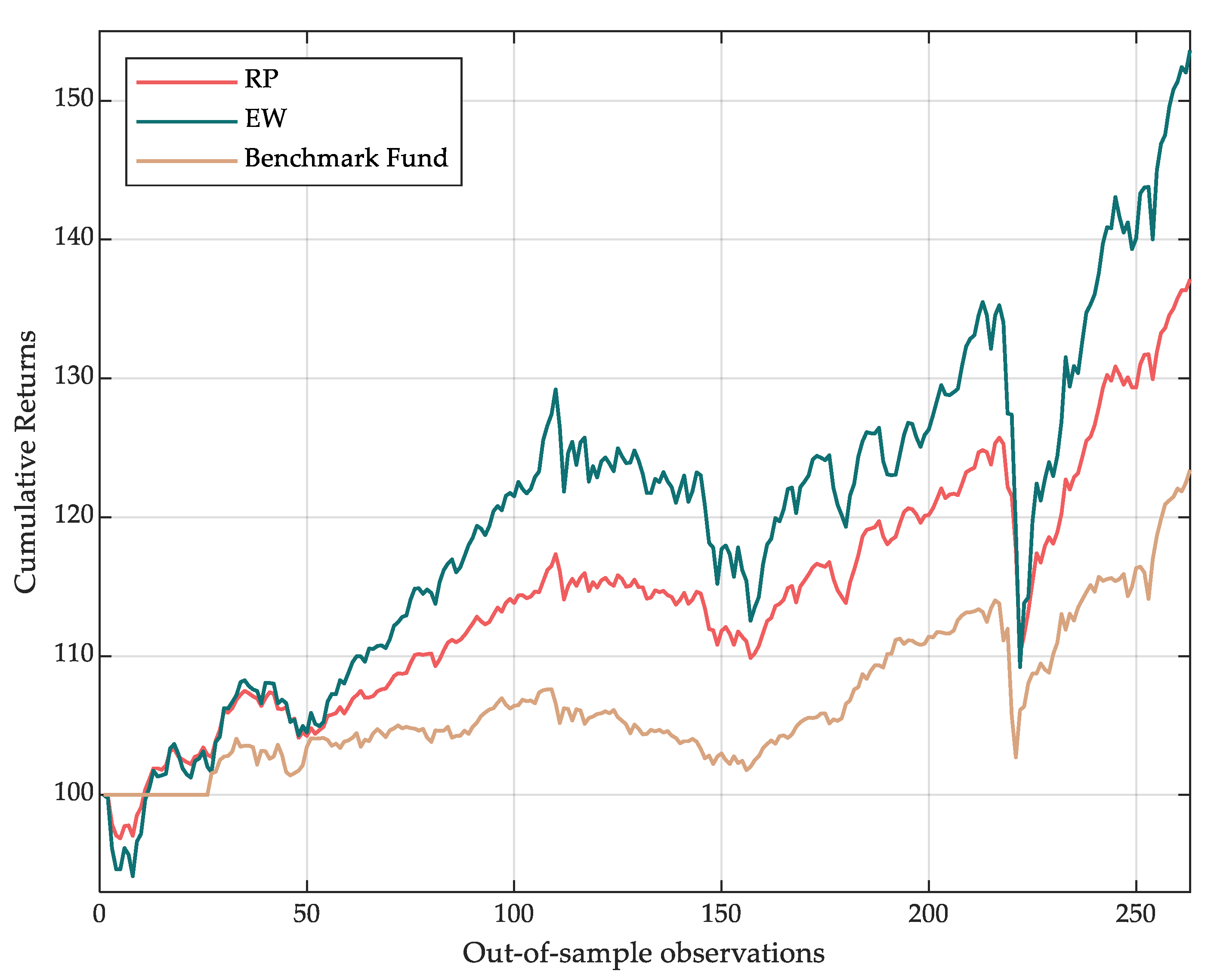
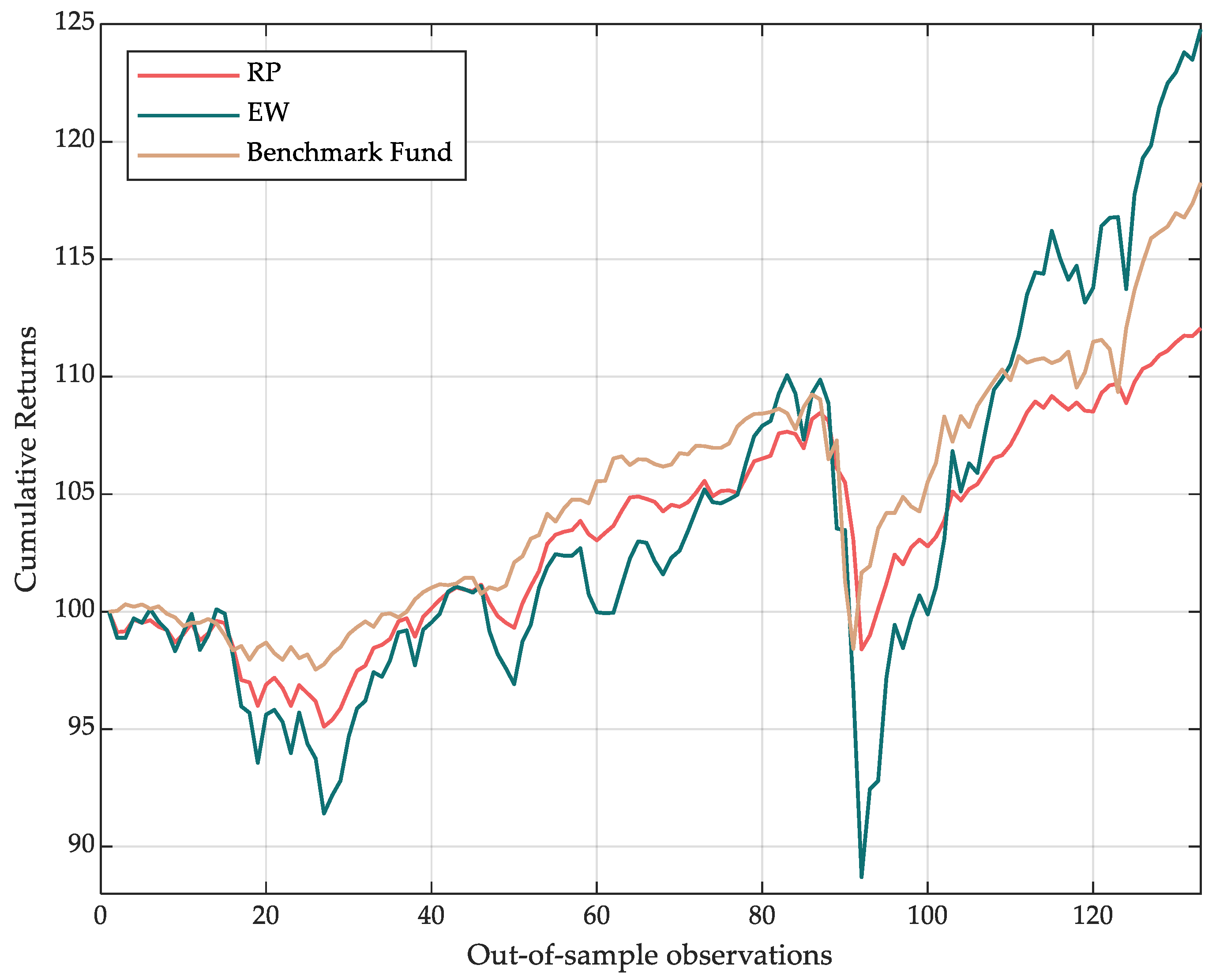
| Return (%) | 8.61 | 6.32 | 4.26 | 9.06 | 4.62 | 6.93 |
| Volatility (%) | 7.34 | 4.49 | 4.98 | 8.88 | 4.04 | 9.06 |
| Sharpe Ratio | 1.17 | 1.41 | 0.86 | 1.02 | 1.14 | 1.11 |
| Max Drawdown (%) | −15.22 | −9.41 | −9.91 | −15.22 | −6.70 | −9.91 |
| Calmar Ratio | 0.57 | 0.67 | 0.43 | 0.59 | 0.69 | 0.70 |
| Downside Risk | 4.41 | 4.37 | 4.84 | 4.21 | 4.39 | 4.39 |
| Sortino Ratio | 1.95 | 1.45 | 0.85 | 2.15 | 1.05 | 1.58 |
| In-Sample w = 244–Out-of-Sample w = 262 | In-Sample w = 130–Out-of-Sample w = 132 | |||||||||
|---|---|---|---|---|---|---|---|---|---|---|
| Min | Max | Mean | Median | Variance | Min | Max | Mean | Median | Variance | |
| SP500 | 3.63% | 6.21% | 5.23% | 5.49% | 0.0055% | 1.63% | 6.12% | 3.94% | 4.60% | 0.0253% |
| MSCIW | 3.88% | 5.74% | 5.04% | 5.14% | 0.0024% | 1.81% | 6.03% | 4.10% | 4.72% | 0.0234% |
| MSCIEM | 3.91% | 4.68% | 4.32% | 4.28% | 0.0004% | 2.31% | 4.82% | 3.83% | 4.30% | 0.0090% |
| MSCIAP | 4.41% | 5.38% | 4.87% | 4.86% | 0.0003% | 2.82% | 5.35% | 4.27% | 4.73% | 0.0083% |
| CONVBOND | 7.30% | 12.67% | 10.89% | 11.25% | 0.0221% | 3.40% | 12.96% | 8.79% | 10.64% | 0.1329% |
| High-Volatility Assets (Total) | 23.14% | 34.68% | 30.36% | 31.03% | 0.0306% | 11.97% | 35.28% | 24.94% | 29.00% | 0.1990% |
| USTREAS | 13.25% | 17.02% | 14.17% | 13.79% | 0.0089% | 12.78% | 55.21% | 25.73% | 13.24% | 3.4703% |
| EUROIL | 12.41% | 17.39% | 14.92% | 14.99% | 0.0057% | 6.12% | 17.38% | 13.25% | 15.93% | 0.2148% |
| EUROGOV | 15.72% | 18.83% | 16.76% | 16.56% | 0.0074% | 11.10% | 18.35% | 15.00% | 16.02% | 0.0517% |
| GOLD | 7.07% | 9.48% | 7.66% | 7.61% | 0.0015% | 4.40% | 11.29% | 7.13% | 7.85% | 0.0241% |
| EURCORP | 14.97% | 18.44% | 16.13% | 15.70% | 0.0099% | 10.55% | 16.19% | 13.93% | 15.07% | 0.0403% |
| In-Sample w = 244–Out-of-Sample w = 262 | In-Sample w = 130–Out-of-Sample w = 132 | |||||||||
|---|---|---|---|---|---|---|---|---|---|---|
| Min | Max | Mean | Median | Variance | Min | Max | Mean | Median | Variance | |
| SP500 | 0.94% | 2.57% | 1.44% | 1.31% | 0.0025% | 0.95% | 4.68% | 2.40% | 1.61% | 0.0206% |
| MSCIW | 1.02% | 2.53% | 1.49% | 1.33% | 0.0022% | 0.98% | 4.53% | 2.31% | 1.52% | 0.0188% |
| MSCIEM | 1.43% | 2.60% | 1.83% | 1.73% | 0.0013% | 1.41% | 4.11% | 2.37% | 1.73% | 0.0107% |
| MSCIAP | 1.19% | 2.34% | 1.56% | 1.49% | 0.0011% | 1.19% | 3.75% | 2.14% | 1.53% | 0.0097% |
| CONVBOND | 0.23% | 0.77% | 0.36% | 0.29% | 0.0003% | 0.27% | 1.42% | 0.68% | 0.39% | 0.0022% |
| High-Volatility Assets (Total) | 4.80% | 10.81% | 6.68% | 6.15% | 0.01% | 4.80% | 18.49% | 9.90% | 6.78% | 0.0620% |
| USTREAS | −0.02% | 0.02% | 0.01% | 0.01% | 0.0000% | −0.05% | 0.01% | −0.01% | 0.00% | 0.0000% |
| EUROIL | 0.08% | 0.36% | 0.16% | 0.13% | 0.0001% | 0.09% | 0.68% | 0.28% | 0.14% | 0.0006% |
| EUROGOV | 0.10% | 0.26% | 0.14% | 0.13% | 0.0000% | 0.05% | 0.40% | 0.19% | 0.13% | 0.0002% |
| GOLD | 0.25% | 0.78% | 0.56% | 0.54% | 0.0001% | 0.00% | 0.86% | 0.58% | 0.54% | 0.0002% |
| EURCORP | 0.05% | 0.20% | 0.08% | 0.06% | 0.0000% | 0.03% | 0.35% | 0.13% | 0.05% | 0.0002% |
| In-Sample w = 244–Out-of-Sample w = 262 | In-Sample w = 130–Out-of-Sample w = 132 | |||||
|---|---|---|---|---|---|---|
| EW | RP | Benchmark Fund | EW | RP | Benchmark Fund | |
| Return (%) | 9.58 | 6.96 | 6.93 | 9.26 | 4.66 | 6.93 |
| Volatility (%) | 9.70 | 5.60 | 9.06 | 11.73 | 5.17 | 6.24 |
| Sharpe Ratio | 0.99 | 1.24 | 1.11 | 0.79 | 0.90 | 1.11 |
| Max Drawdown (%) | −19.41 | −12.36 | −9.91 | −19.41 | −9.27 | −9.91 |
| Calmar Ratio | 0.49 | 0.56 | 0.70 | 0.48 | 0.50 | 0.70 |
| Downside Risk | 4.57 | 4.34 | 4.39 | 4.53 | 4.35 | 4.39 |
| Sortino Ratio | 2.10 | 1.60 | 1.58 | 2.05 | 1.07 | 1.58 |
| In-Sample w = 244–Out-of-Sample w = 262 | In-Sample w = 130–Out-of-Sample w = 132 | |||||||||
|---|---|---|---|---|---|---|---|---|---|---|
| Min | Max | Mean | Median | Variance | Min | Max | Mean | Median | Variance | |
| SP500 | 3.03% | 4.58% | 3.62% | 3.45% | 0.0020% | 1.40% | 4.95% | 2.67% | 2.77% | 0.0083% |
| MSCIW | 2.89% | 4.29% | 3.44% | 3.28% | 0.0019% | 1.52% | 4.92% | 2.81% | 3.01% | 0.0072% |
| MSCIEM | 2.38% | 3.62% | 2.99% | 2.80% | 0.0014% | 2.02% | 3.68% | 2.70% | 2.80% | 0.0016% |
| MSCIAP | 2.81% | 4.17% | 3.48% | 3.32% | 0.0017% | 2.32% | 4.10% | 2.97% | 3.05% | 0.0017% |
| CONVBOND | 7.51% | 12.85% | 10.54% | 10.90% | 0.0230% | 3.43% | 13.08% | 8.06% | 8.81% | 0.1023% |
| MSCIWI | 2.88% | 4.26% | 3.45% | 3.34% | 0.0019% | 1.64% | 4.82% | 2.80% | 2.84% | 0.0061% |
| SPS500 | 2.92% | 4.56% | 3.62% | 3.46% | 0.0023% | 1.43% | 4.89% | 2.62% | 2.78% | 0.0072% |
| MSCIEMI | 2.39% | 3.60% | 2.96% | 2.70% | 0.0019% | 1.94% | 3.60% | 2.53% | 2.54% | 0.0014% |
| MSCIAPI | 2.84% | 4.25% | 3.47% | 3.32% | 0.0016% | 2.14% | 3.99% | 2.73% | 2.73% | 0.0016% |
| High-Volatility Assets (Total) | 29.64% | 46.19% | 37.57% | 36.57% | 0.0377% | 17.84% | 48.03% | 29.88% | 31.32% | 0.1375% |
| USTREAS | 9.44% | 14.09% | 12.19% | 12.80% | 0.0184% | 9.89% | 45.52% | 21.91% | 12.97% | 2.0204% |
| EUROIL | 12.08% | 15.64% | 14.05% | 14.15% | 0.0098% | 6.25% | 16.68% | 12.69% | 14.90% | 0.1775% |
| EUROGOV | 12.10% | 16.50% | 14.75% | 15.18% | 0.0186% | 11.87% | 17.14% | 14.89% | 15.00% | 0.0224% |
| GOLD | 5.90% | 10.98% | 7.55% | 6.71% | 0.0165% | 5.68% | 14.63% | 6.93% | 6.76% | 0.0138% |
| EURCORP | 10.85% | 16.09% | 13.89% | 14.55% | 0.0229% | 11.08% | 16.33% | 13.69% | 13.98% | 0.0203% |
| In-Sample w = 244–Out-of-Sample w = 262 | In-Sample w = 130–Out-of-Sample w = 132 | |||||||||
|---|---|---|---|---|---|---|---|---|---|---|
| Min | Max | Mean | Median | Variance | Min | Max | Mean | Median | Variance | |
| SP500 | 0.97% | 2.63% | 1.49% | 1.37% | 0.0026% | 0.98% | 4.86% | 2.50% | 1.71% | 0.0220% |
| MSCIW | 1.07% | 2.62% | 1.56% | 1.39% | 0.0023% | 1.03% | 4.75% | 2.44% | 1.63% | 0.0205% |
| MSCIEM | 1.51% | 2.70% | 1.92% | 1.82% | 0.0013% | 1.52% | 4.27% | 2.51% | 1.87% | 0.0110% |
| MSCIAP | 1.24% | 2.45% | 1.63% | 1.55% | 0.0013% | 1.26% | 3.96% | 2.27% | 1.63% | 0.0108% |
| CONVBOND | 0.17% | 0.64% | 0.28% | 0.23% | 0.0002% | 0.19% | 1.23% | 0.56% | 0.33% | 0.0015% |
| MSCIWI | 1.08% | 2.56% | 1.56% | 1.41% | 0.0021% | 1.05% | 4.61% | 2.41% | 1.66% | 0.0186% |
| SPS500 | 1.00% | 2.59% | 1.51% | 1.40% | 0.0024% | 1.02% | 4.76% | 2.51% | 1.77% | 0.0201% |
| MSCIEMI | 1.49% | 2.73% | 1.93% | 1.85% | 0.0014% | 1.52% | 4.36% | 2.59% | 1.98% | 0.0113% |
| MSCIAPI | 1.18% | 2.51% | 1.62% | 1.57% | 0.0016% | 1.29% | 4.15% | 2.39% | 1.75% | 0.0118% |
| High-Volatility Assets (Total) | 9.73% | 21.43% | 13.49% | 12.57% | 0.0152% | 9.87% | 36.97% | 20.17% | 14.31% | 0.1277% |
| USTREAS | −0.02% | 0.01% | 0.00% | 0.01% | 0.0000% | −0.06% | 0.01% | −0.02% | 0.00% | 0.0000% |
| EUROIL | 0.04% | 0.28% | 0.10% | 0.07% | 0.0001% | 0.05% | 0.54% | 0.22% | 0.09% | 0.0004% |
| EUROGOV | 0.05% | 0.19% | 0.10% | 0.09% | 0.0000% | 0.01% | 0.31% | 0.14% | 0.09% | 0.0001% |
| GOLD | 0.04% | 0.47% | 0.32% | 0.31% | 0.0000% | −0.21% | 0.43% | 0.32% | 0.33% | 0.0000% |
| EURCORP | 0.05% | 0.20% | 0.08% | 0.06% | 0.0000% | 0.03% | 0.35% | 0.13% | 0.05% | 0.0002% |
Publisher’s Note: MDPI stays neutral with regard to jurisdictional claims in published maps and institutional affiliations. |
© 2021 by the authors. Licensee MDPI, Basel, Switzerland. This article is an open access article distributed under the terms and conditions of the Creative Commons Attribution (CC BY) license (https://creativecommons.org/licenses/by/4.0/).
Share and Cite
Delle Foglie, A.; Pola, G. Make the Best from Comparing Conventional and Islamic Asset Classes: A Design of an All-Seasons Combined Portfolio. J. Risk Financial Manag. 2021, 14, 484. https://doi.org/10.3390/jrfm14100484
Delle Foglie A, Pola G. Make the Best from Comparing Conventional and Islamic Asset Classes: A Design of an All-Seasons Combined Portfolio. Journal of Risk and Financial Management. 2021; 14(10):484. https://doi.org/10.3390/jrfm14100484
Chicago/Turabian StyleDelle Foglie, Andrea, and Gianni Pola. 2021. "Make the Best from Comparing Conventional and Islamic Asset Classes: A Design of an All-Seasons Combined Portfolio" Journal of Risk and Financial Management 14, no. 10: 484. https://doi.org/10.3390/jrfm14100484
APA StyleDelle Foglie, A., & Pola, G. (2021). Make the Best from Comparing Conventional and Islamic Asset Classes: A Design of an All-Seasons Combined Portfolio. Journal of Risk and Financial Management, 14(10), 484. https://doi.org/10.3390/jrfm14100484