
Causality between Energy Consumption and Economic Growth in the Presence of Growth Volatility: Multi-Country Evidence


Abstract
1. Introduction
2. Literature Review
3. Data and Methods
4. Results and Discussion
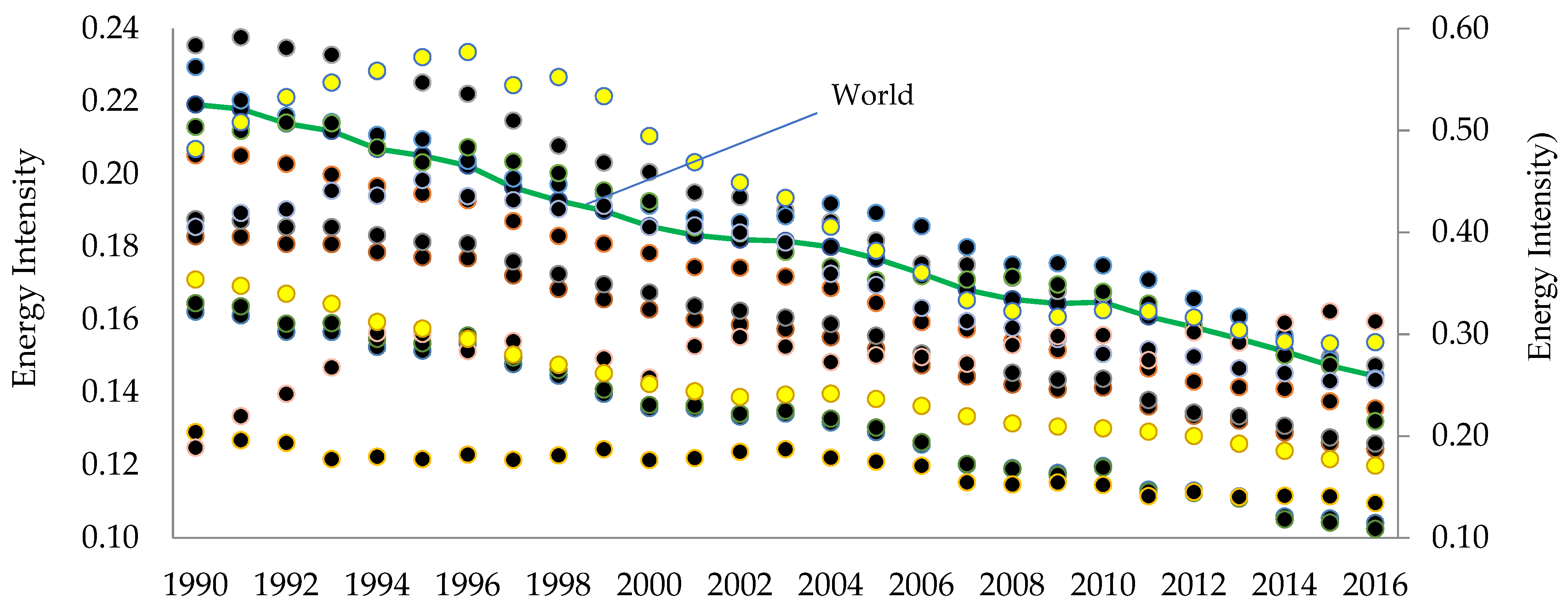
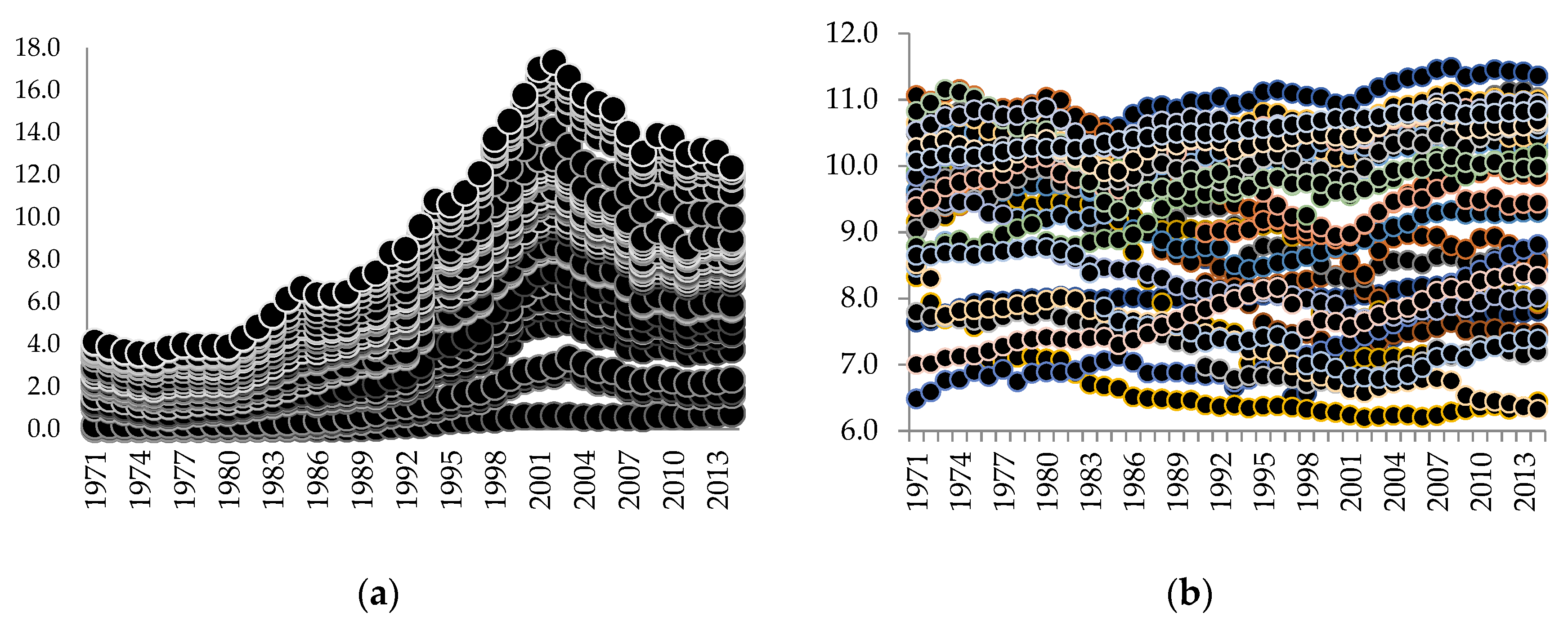
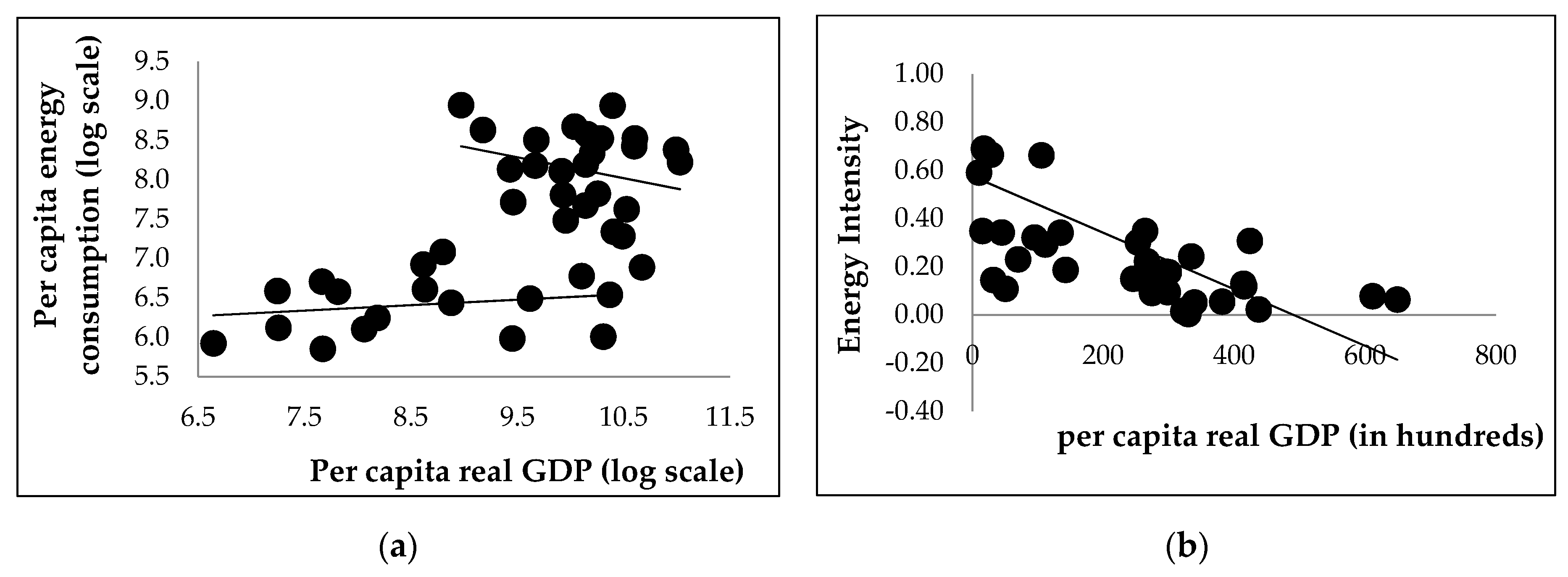
4.1. Descriptive Evidence
4.2. Unit Roots and Cointegration
4.3. Long-Run Causal Inferences
4.4. Short-Run Causal Inferences
5. Concluding Remarks and Policy Implications
Author Contributions
Funding
Data Availability Statement
Acknowledgments
Conflicts of Interest
Appendix A

| Countries | Level | First Difference | ||||||||
|---|---|---|---|---|---|---|---|---|---|---|
| ADF | PP | KPSS | Breakpoint | Break | ADF | PP | KPSS | Breakpoint | Break | |
| Albania | −2.36 | −1.42 | 0.16 ** | −3.79 | 2003 | −3.79 *** | −3.03 *** | 0.32 | −5.29 ** | 1990 |
| Algeria | −2.63 | −1.66 | 0.15 ** | −3.02 | 1990 | −2.98 ** | −4.52 *** | 0.15 | −4.64 ** | 1979 |
| Australia | −1.74 | −1.99 | 0.19 ** | −3.55 | 2000 | −5.35 *** | −5.35 *** | 0.11 | −6.33 *** | 2001 |
| Austria | −2.11 | −1.44 | 0.18 ** | −2.37 | 1981, 1986 | −3.02 ** | −3.17 ** | 0.19 | −8.97 *** | 1985 |
| Bangladesh | −2.47 | −2.04 | 0.14 * | −3.72 | 2003 | −4.59 *** | −4.59 *** | 0.08 | −4.81 ** | 2002 |
| Belgium | −1.01 | −0.89 | 0.15 ** | −3.63 | 1980 | −3.05 ** | −3.08 ** | 0.26 | −6.94 *** | 2000 |
| Bolivia | −2.16 | −2.27 | 0.17 ** | −2.02 | 1999 | −4.29 *** | −4.35 *** | 0.19 | −4.89 ** | 2003 |
| Brazil | −2.53 | −2.13 | 0.14 * | −3.88 | 1986 | −4.25 *** | −4.24 *** | 0.09 | −4.77 ** | 1985 |
| Canada | −2.35 | −2.27 | 0.17 ** | −3.35 | 1992 | −4.65 *** | −4.66 *** | 0.08 | −5.69 *** | 1975 |
| Chile | −2.32 | −2.57 | 0.18 ** | −3.32 | 1997 | −6.95 *** | −6.95 *** | 0.07 | −16.87 *** | 1998 |
| China | −2.34 | −2.25 | 0.18 ** | −3.01 | 1986 | −6.33 *** | −6.34 *** | 0.19 | −9.92 *** | 1992 |
| Colombia | −1.68 | −1.65 | 0.17 ** | −3.11 | 1992 | −4.54 *** | −4.56 *** | 0.18 | −5.89 *** | 1993 |
| The Czech Republic | −2.08 | −1.36 | 0.15 ** | −2.71 | 1985 | −4.53 *** | −4.53 *** | 0.23 | −5.06 *** | 2012 |
| Denmark | −2.52 | −2.34 | 0.14 * | −2.68 | 1980 | −4.79 *** | −4.69 *** | 0.13 | −5.37 *** | 1985 |
| Ecuador | −2.39 | −1.74 | 0.12 * | −3.26 | 1987 | −2.91 * | −3.13 ** | 0.16 | −4.31 * | 1979 |
| Egypt | −1.71 | −1.82 | 0.16 ** | −3.73 | 1985 | −4.25 *** | −4.36 *** | 0.16 | −4.94 ** | 1994 |
| Finland | −1.44 | −1.48 | 0.14 * | −2.93 | 1982 | −4.31 *** | −4.44 *** | 0.19 | −6.34 *** | 1986 |
| France | −2.66 | −2.27 | 0.17 ** | −2.22 | 2004 | −4.66 *** | −4.66 *** | 0.06 | −5.25 *** | 1986 |
| Gabon | −1.8 | −1.8 | 0.22 *** | −2.92 | 1986 | −5.95 *** | −6.11 *** | 0.29 | −7.11 *** | 1983 |
| Germany | −1.93 | −1.21 | 0.21 *** | −3.05 | 1985 | −4.92 *** | −4.84 *** | 0.31 | −5.55 *** | 1981 |
| Hungary | −2.99 | −2.06 | 0.12 * | −3.43 | 1985 | −4.47 *** | −4.37 *** | 0.14 | −4.92 ** | 1992 |
| India | −0.58 | −0.26 | 0.22 ** | −3.94 | 1974 | −4.91 *** | −4.61 *** | 0.13 | −7.43 *** | 1975 |
| Indonesia | −1.93 | −1.37 | 0.12 * | −4.11 | 1987 | −2.92 * | −2.97 ** | 0.21 | −4.29 * | 1994 |
| Iran | −1.88 | −0.82 | 0.23 *** | −2.88 | 1978 | −3.26 ** | −2.64 * | 0.31 | −5.23 *** | 1978 |
| Italy | −0.89 | −1.05 | 0.16 ** | −1.04 | 2001 | −2.86 * | −5.25 *** | 0.3 | −5.89 *** | 1996 |
| Japan | −1.75 | −3.33 * | 0.15 ** | −2.92 | 2004 | −6.64 *** | −6.37 *** | 0.25 | −7.55 *** | 2008 |
| Korea South | −3.12 | −2.17 | 0.14 * | −4.12 | 1985 | −4.81 *** | −4.71 *** | 0.31 | −5.42 *** | 1981 |
| The Netherlands | −3.38 * | −2.58 | 0.15 ** | −3.71 | 1985 | −5.00 *** | −4.86 *** | 0.08 | −5.53 *** | 1981 |
| New Zealand | −3.11 | −2.58 | 0.12 * | −3.58 | 2000 | −4.22 *** | −4.13 *** | 0.06 | −4.62 *** | 1999 |
| Nigeria | −3.11 | −2.32 | 0.16 ** | −3.89 | 1984 | −4.81 *** | −4.54 *** | 0.08 | −5.88 *** | 1993 |
| Norway | −3.11 | −2.51 | 0.15 ** | −3.57 | 1985 | −4.97 *** | −4.92 *** | 0.09 | −5.34 **** | 1981 |
| Pakistan | −2.26 | −2.07 | 0.13 * | − | − | −2.92 * | −2.84 * | 0.28 | − | − |
| Philippines | −0.78 | −0.99 | 0.16 ** | −2.77 | 1988 | −5.89 *** | −6.03 *** | 0.24 | −7.46 *** | 1991 |
| Portugal | −3.03 | −2.5 | 0.18 ** | −3.72 | 1980 | −4.95 *** | −4.73 *** | 0.06 | −6.29 *** | 1986 |
| South Africa | −1.38 | −0.47 | 0.24 *** | −3.42 | 1985 | −5.03 *** | −4.83 *** | 0.33 | −5.77 *** | 1995 |
| Spain | −5.61 *** | −5.52 *** | 0.05 | −4.69 ** | 1986 | − | − | − | − | − |
| Sri Lanka | −0.64 | −0.71 | 0.19 ** | −2.56 | 1978 | −6.81 *** | −6.89 *** | 0.32 | −11.02 *** | 1978 |
| Sudan | −2.51 | −1.81 | 0.15 ** | −3.71 | 1985 | −4.94 *** | −4.87 *** | 0.18 | −5.54 *** | 1981 |
| Sweden | −2.98 | −2.14 | 0.19 ** | −3.92 | 2000 | −4.28 *** | −4.32 *** | 0.24 | −4.84 ** | 1984 |
| Syrian | −3.06 | −3.05 | 0.13 ** | −1.71 | 1982 | −5.27 *** | −5.11 *** | 0.07 | −8.53 *** | 1973 |
| Thailand | −1.39 | −1.09 | 0.17 ** | −2.79 | 1981 | −4.49 *** | −4.52 *** | 0.32 | −5.94 *** | 1984 |
| Trinidad and Tobago | −2.29 | −1.95 | 0.12 * | −3.34 | 1979 | −3.74 *** | −3.74 *** | 0.12 | −4.74 ** | 1980 |
| Turkey | −3.05 | −2.58 | 0.13 * | −3.38 | 2001 | −5.26 *** | −5.08 *** | 0.05 | −5.69 *** | 1992 |
| UAE | −2.79 | −2.38 | 0.12 * | −2.45 | 1986 | −4.91 *** | −4.95 *** | 0.06 | 7.46 *** | 1998 |
| UK | −2.34 | −1.66 | 0.13 * | −3.17 | 1979 | −2.82 * | −3.79 *** | 0.19 | 5.23 *** | 2001 |
| USA | −3.01 | −2.62 | 0.15 ** | −3.56 | 1992 | −4.29 *** | −3.74 *** | 0.07 | −6.29 *** | 2008 |
| Venezuela | −2.19 | −1.24 | 0.21 ** | −3.81 | 1982 | −5.03 *** | −4.80 *** | 0.27 | −5.73 *** | 2009 |
| Vietnam | −2.09 | −2.3 | 0.15 ** | − | − | −2.66 * | −2.72 * | 0.31 | − | − |
| Countries | Level | First Difference | ||||||||
|---|---|---|---|---|---|---|---|---|---|---|
| ADF | PP | KPSS | Breakpoint | Break | ADF | PP | KPSS | Breakpoint | Break | |
| Albania | −1.27 | −1.50 | 0.15 ** | −2.29 | 1989 | −6.18 *** | −6.20 *** | 0.14 | −7.65 *** | 1992 |
| Algeria | −2.94 | −2.92 | 0.16 ** | −4.08 | 2002 | −4.29 *** | −5.07 *** | 0.25 | −7.55 *** | 1982 |
| Australia | −1.43 | −1.29 | 0.21 ** | −4.12 | 1993 | −7.65 *** | −7.61 *** | 0.31 | −8.67 *** | 2007 |
| Austria | −1.83 | −1.83 | 0.21 ** | −3.06 | 1,995 | −6.72 *** | −6.74 *** | 0.31 | −8.11 *** | 1972 |
| Bangladesh | −0.93 | −0.62 | 0.20 ** | −0.69 | 2000 | −8.18 *** | −8.18 *** | 0.28 | −9.16 *** | 2001 |
| Belgium | −1.61 | −1.62 | 0.19 ** | −3.53 | 2012 | −6.61 *** | −6.61 *** | 0.32 | −7.29 *** | 1972 |
| Bolivia | −2.74 | −2.82 | 0.16 ** | −2.61 | 1993 | −7.74 *** | −7.63 *** | 0.11 | −8.36 *** | 2001 |
| Brazil | −1.61 | −2.06 | 0.15 ** | −2.54 | 2003 | −5.59 *** | −5.59 *** | 0.13 | −6.51 *** | 1981 |
| Canada | −2.13 | −2.11 | 0.22 *** | − | − | −4.77 *** | −4.57 *** | 0.35 * | − | − |
| Chile | −3.02 | −2.66 | 0.15 ** | −3.34 | 1987 | −4.52 *** | −4.48 *** | 0.27 | −5.58 *** | 1975 |
| China | −1.35 | −0.88 | 0.19 ** | −3.28 | 2002 | −3.57 ** | −3.57 ** | 0.31 | −4.49 ** | 2001 |
| Colombia | −1.76 | −1.86 | 0.17 ** | −1.97 | 1984 | −7.17 *** | −7.14 *** | 0.09 | −8.18 *** | 1999 |
| The Czech Republic | −2.17 | −2.27 | 0.18 ** | −3.45 | 1990 | −7.12 *** | −7.12 *** | 0.08 | −7.45 *** | 1999 |
| Denmark | −2.96 | −2.97 | 0.20 ** | −3.57 | 2009 | −7.18 *** | −7.14 *** | 0.09 | −8.18 *** | 1999 |
| Ecuador | −2.78 | −2.72 | 0.15 ** | −3.07 | 1995 | −7.32 *** | −7.45 *** | 0.15 | −7.81 *** | 1985 |
| Egypt | −1.09 | −1.18 | 0.15 ** | −2.73 | 2001 | −5.58 *** | −5.17 *** | 0.37 * | −6.42 *** | 1985 |
| Finland | −1.35 | −1.07 | 0.23 *** | − | − | −7.27 *** | −7.33 *** | 0.28 | − | − |
| France | −1.46 | −1.45 | 0.23 *** | − | − | −6.15 *** | −6.14 *** | 0.29 | − | − |
| Gabon | −1.07 | −1.08 | 0.19 ** | −2.23 | 2001 | −5.99 *** | −6.00 *** | 0.21 | −6.61 *** | 1976 |
| Germany | −1.96 | −1.96 | 0.23 *** | −3.28 | 2008 | −5.86 *** | −5.82 *** | 0.27 | −11.34 *** | 1972 |
| Hungary | −1.97 | −1.97 | 0.21 ** | −3.56 | 2008 | −4.68 *** | −4.66 *** | 0.18 | −6.83 *** | 1973 |
| India | −0.21 | −0.38 | 0.18 ** | −0.49 | 2005 | −4.81 *** | −5.04 *** | 0.17 | −7.19 *** | 2003 |
| Indonesia | −1.24 | −1.24 | 0.15 ** | −3.16 | 1999 | −6.58 *** | −6.58 *** | 0.19 | −8.50 *** | 1990 |
| Iran | −3.33 | −3.25 | 0.16 ** | −3.59 | 1988 | −8.34 *** | −8.16 *** | 0.15 | −10.28 *** | 1977 |
| Italy | −3.11 | −3.12 | 0.20 ** | −2.26 | 1995 | −6.29 *** | −6.35 *** | 0.27 | −7.99 *** | 2007 |
| Japan | −2.78 | −2.52 | 0.21 ** | −2.61 | 2008 | −5.85 *** | −5.85 *** | 0.32 | −7.36 *** | 1972 |
| Korea South | −0.19 | −0.17 | 0.21 ** | −2.65 | 1985 | −5.34 *** | −5.42 *** | 0.28 | 7.64 *** | 1998 |
| The Netherlands | −2.29 | −2.27 | 0.19 ** | − | − | −5.83 *** | −5.84 *** | 0.32 | − | − |
| New Zealand | −2.06 | −1.98 | 0.24 *** | −3.59 | 1983 | −7.37 *** | −7.37 *** | 0.33 | −8.368 *** | 1979 |
| Nigeria | −2.63 | −2.46 | 0.18 ** | −3.04 | 1998 | −5.51 *** | −5.44 *** | 0.24 | −6.42 *** | 1994 |
| Norway | −1.97 | −1.73 | 0.25 *** | − | − | −9.44 *** | −9.91 *** | 0.36 * | − | − |
| Pakistan | −1.87 | −1.88 | 0.18 ** | −3.21 | 1986 | −5.16 *** | −5.18 *** | 0.33 | −7.33 *** | 2007 |
| Philippines | −2.49 | −2.53 | 0.15 ** | −3.11 | 1985 | −8.63 *** | −8.33 *** | 0.09 | −8.97 *** | 2009 |
| Portugal | −0.16 | −0.16 | 0.22 *** | − | − | −5.41 *** | −5.44 *** | 0.26 | − | − |
| South Africa | −1.98 | −1.95 | 0.16 ** | −2.61 | 2002 | −6.22 *** | −6.23 *** | 0.16 | −6.87 *** | 2007 |
| Spain | −0.75 | −0.91 | 0.22 *** | − | − | −4.31 *** | −4.39 *** | 0.26 | − | − |
| Sri Lanka | −2.28 | −2.08 | 0.18 ** | −2.99 | 1994 | −7.32 *** | −7.45 *** | 0.21 | −8.18 *** | 1996 |
| Sudan | −2.97 | −2.85 | 0.17 ** | −3.24 | 1985 | −7.01 *** | −11.08 *** | 0.29 | −10.18 *** | 2002 |
| Sweden | −2.13 | −2.13 | 0.25 *** | −3.45 | 2008 | −8.37 *** | −8.45 *** | 0.31 | −9.15 *** | 1985 |
| Syrian | −0.26 | −0.51 | 0.21 ** | −1.98 | 2004 | −5.49 *** | −5.55 *** | 0.35 * | −6.75 *** | 2005 |
| Thailand | −1.91 | −2.01 | 0.19 ** | −3.24 | 1986 | −4.88 *** | 4.98 *** | 0.09 | −6.21 *** | 1983 |
| Trinidad and Tobago | −2.19 | −2.21 | 0.19 ** | −2.35 | 1995 | −3.47 ** | −6.33 *** | 0.15 | −7.38 *** | 1978 |
| Turkey | −2.52 | −2.57 | 0.17 ** | −1.79 | 2002 | −6.42 *** | −6.42 *** | 0.09 | −7.35 *** | 1999 |
| UAE | −0.89 | −0.83 | 0.21 ** | −2.63 | 2003 | −6.39 *** | −6.42 *** | 0.19 | −7.99 *** | 1987 |
| UK | −0.54 | −0.35 | 0.19 ** | −2.92 | 2008 | −7.27 *** | −7.24 *** | 0.13 | −8.57 *** | 2005 |
| USA | −2.62 | −1.92 | 0.19 ** | −4.07 | 2008 | −5.05 *** | −4.94 *** | 0.29 | −5.56 *** | 1978 |
| Venezuela | −2.92 | −2.97 | 0.15 ** | −3.57 | 2004 | −10.98 *** | −10.46 *** | 0.31 | −13.16 *** | 1991 |
| Vietnam | −1.74 | −1.75 | 0.22 *** | −1.96 | 1996 | −5.32 *** | −5.51 *** | 0.32 | 7.43 *** | 1992 |
| Countries | Model | ADF | PP | KPSS | Breakpoint | Break |
|---|---|---|---|---|---|---|
| Albania | EGARCH(1,1) | −3.77 ** | −3.57 ** | 0.07 | −7.64 *** | 2002 |
| Algeria | EGARCH(1,1) | −4.51 *** | −5.80 *** | 0.07 | −5.20 *** | 1992 |
| Australia | EGARCH(3,0) | −6.74 *** | −8.08 *** | 0.19 | −12.26 *** | 2010 |
| Austria | EGARCH(1,0) | −5.14 *** | −5.15 *** | 0.1 | −23.59 *** | 1985, 1990 |
| Bangladesh | EGARCH(1,2) | −7.47 *** | −5.56 *** | 0.08 | −9.71 *** | 2001 |
| Belgium | EGARCH(1,0) | −4.59 *** | −4.65 *** | 0.06 | −6.01 *** | 2004 |
| Bolivia | EGARCH(1,0) | −4.81 *** | −4.48 *** | 0.1 | −5.09 *** | 1976 |
| Brazil | EGARCH(2,1) | −3.11 ** | −4.04 *** | 0.1 | −4.45 ** | 1994 |
| Canada | EGARCH(1.0) | −5.37 *** | −5.22 *** | 0.15 | −10.46 *** | 1995 |
| Chile | EGARCH(2,2) | −2.97 ** | −2.92 ** | 0.11 | −5.06 *** | 2001 |
| China | EGARCH(2,2) | −5.71 *** | −5.53 *** | 0.14 | −13.30 *** | 1992, 1999 |
| Colombia | EGARCH(1,0) | −5.76 *** | −5.77 *** | 0.17 | −14.09 *** | 1994, 1997 |
| The Czech Republic | EGARCH(1,2) | −3.72 *** | −3.81 *** | 0.22 | − | − |
| Denmark | EGARCH(2,2) | −6.74 *** | −8.11 *** | 0.12 | −8.44 *** | 2004 |
| Ecuador | EGARCH(2,2) | −4.92 *** | −5.42 *** | 0.21 | −4.64 ** | 1982, 1990 |
| Egypt | EGARCH(3,0) | −5.23 *** | −5.13 *** | 0.09 | −7.07 *** | 1996 |
| Finland | EGARCH(1,1) | −8.84 *** | −8.77 *** | 0.17 | −10.96 *** | 1985, 1991 |
| France | EGARCH(1,0) | −6.67 *** | −6.66 *** | 0.31 | −8.92 *** | 1991, 2010 |
| Gabon | EGARCH(1,1) | −12.53 *** | −11.76 *** | 0.08 | −14.89 *** | 1987, 1997, 2003 |
| Germany | EGARCH(2,2) | −4.09 *** | −3.17 ** | 0.21 | −4.49 ** | 1994 |
| Hungary | EGARCH(2,2) | 10.31 *** | −9.74 *** | 0.35 * | −14.61 *** | 1978 |
| India | EGARCH(1,2) | −6.56 *** | −7.92 *** | 0.28 | −6.95 *** | 1975, 1981 |
| Indonesia | EGARCH(1,1) | −2.93 ** | 3.87 *** | 0.14 | −5.45 *** | 1983, 1992 |
| Iran | EGARCH(1,1) | −3.04 ** | −3.19 ** | 0.23 | −11.73 *** | 1975, 1978 |
| Italy | EGARCH(1,0) | −5.83 *** | −5.72 *** | 0.28 | −6.29 *** | 1988 |
| Japan | EGARCH(1,1) | −6.73 *** | −6.38 *** | 0.1 | 7.26 *** | 2008 |
| Korea South | EGARCH(1,0) | −6.62 *** | −6.62 *** | 0.13 | −6.91 *** | 1987, 2010 |
| The Netherlands | EGARCH(2,0) | −7.84 *** | 11.11 *** | 0.14 | −11.09 *** | 1989, 1992 |
| New Zealand | EGARCH(2,2) | 3.02 ** | −3.07 ** | 0.14 | −5.67 *** | 1981 |
| Nigeria | EGARCH(2,2) | −3.99 *** | −10.23 *** | 0.11 | −11.53 *** | 1980 |
| Norway | EGARCH(1,3) | −7.79 *** | −8.88 *** | 0.22 | − | − |
| Pakistan | EGARCH(1,0) | −4.39 *** | −4.38 *** | 0.11 | −4.78 *** | 2004 |
| Philippines | EGARCH(1,0) | −6.22 *** | −6.36 *** | 0.16 | −7.01 *** | 1986, 2004 |
| Portugal | EGARCH(2,2) | −11.18 *** | −10.89 *** | 0.08 | −13.18 *** | 1979 |
| South Africa | EGARCH(1,1) | −3.09 ** | −3.14 ** | 0.34 | −4.51 ** | 2002 |
| Spain | EGARCH(2,2) | −8.99 *** | −5.92 *** | 0.28 | −10.33 *** | 1999 |
| Sri Lanka | EGARCH(2,2) | −7.81 *** | −7.19 *** | 0.18 | −14.58 *** | 1978 |
| Sudan | EGARCH(3,0) | −7.92 *** | −10.49 *** | 0.24 | −9.47 *** | 2000 |
| Sweden | EGARCH(1,0) | −6.07 *** | −6.08 *** | 0.19 | −6.91 *** | 2004 |
| Syrian | EGARCH(1,0) | −6.55 *** | −6.54 *** | 0.14 | −33.61 *** | 1975 |
| Thailand | EGARCH(1,0) | −7.55 *** | −7.61 *** | 0.19 | −8.28 *** | 1985 |
| Trinidad and Tobago | EGARCH(1,1) | −2.65 * | −2.92 *** | 0.18 | −4.96 *** | 1982 |
| Turkey | EGARCH(2,0) | −3.75 *** | −3.75 *** | 0.26 | −4.73 *** | 1978 |
| UAE | EGARCH(1,0) | −4.84 *** | −4.80 *** | 0.21 | −12.85 *** | 1999 |
| UK | EGARCH(1,0) | −5.94 *** | −5.95 *** | 0.12 | −6.35 *** | 1995 |
| USA | EGARCH(2,1) | −3.11 ** | −3.22 ** | 0.41 * | −5.27 *** | 1975 |
| Venezuela | EGARCH(2,0) | −4.73 *** | −3.24 ** | 0.09 | −5.34 *** | 1983 |
| Vietnam | EGARCH(2,2) | −14.41 *** | −13.36 *** | 0.34 | −54.22 *** | 1997 |
| Countries | Model | ADF | PP | KPSS | Breakpoint | Break |
|---|---|---|---|---|---|---|
| Albania | EGARCH(1,1) | −8.26 *** | −8.43 *** | 0.21 | −14.68 *** | 1992 |
| Algeria | EGARCH(1,1) | −4.08 *** | −2.53 ** | 0.31 | 7.56 *** | 1995 |
| Australia | EGARCH(1,0) | −6.99 *** | −6.98 *** | 0.08 | −7.57 *** | 2011 |
| Austria | EGARCH(1,1) | −3.60 ** | −3.55 ** | 0.23 | −5.07 *** | 2004 |
| Bangladesh | EGARCH(1,1) | −3.98 *** | −3.98 *** | 0.09 | −5.02 *** | 2011 |
| Belgium | EGARCH(1,1) | −6.09 *** | −6.29 *** | 0.24 | −6.99 *** | 1982 |
| Bolivia | EGARCH(1,0) | −6.69 *** | −8.78 *** | 0.27 | 7.07 *** | 1999 |
| Brazil | EGARCH(3,0) | −3.91 *** | −3.82 *** | 0.15 | −5.83 *** | 1982 |
| Canada | EGARCH(1,1) | −3.65 *** | −3.69 *** | 0.21 | −5.13 *** | 1981 |
| Chile | EGARCH(1,1) | −9.72 *** | −9.75 *** | 0.13 | −11.29 *** | 2012 |
| China | EGARCH(1,0) | −5.99 *** | −5.85 *** | 0.18 | −7.21 *** | 2004 |
| Colombia | EGARCH(4,0) | −6.82 *** | −6.97 *** | 0.11 | −15.35 *** | 1980 |
| The Czech Republic | EGARCH(2,2) | −9.99 *** | −12.01 *** | 0.11 | −11.97 *** | 1993 |
| Denmark | EGARCH(1,1) | −4.76 *** | −4.79 *** | 0.19 | −5.74 *** | 1996 |
| Ecuador | EGARCH(2,2) | −7.47 *** | −7.46 *** | 0.17 | −10.01 *** | 2000 |
| Egypt | EGARCH(2,2) | −10.86 *** | 10.24 *** | 0.25 | −11.91 *** | 1985 |
| Finland | EGARCH(2,1) | −10.15 *** | −10.16 *** | 0.09 | −10.21 *** | 1987 |
| France | EGARCH(1,1) | −4.28 *** | −4.31 *** | 0.16 | −5.68 *** | 1978 |
| Gabon | EGARCH(2,1) | −7.88 *** | −8.08 *** | 0.19 | −14.26 *** | 1975 |
| Germany | EGARCH(3,0) | −6.64 *** | −6.64 *** | 0.29 | −46.67 *** | 1974 |
| Hungary | EGARCH(2,0) | −4.46 *** | −4.47 *** | 0.12 | −5.16 *** | 1993 |
| India | EGARCH(2,2) | −6.62 *** | −8.05 *** | 0.15 | −8.11 *** | 2010 |
| Indonesia | EGARCH(1,1) | −3.22 ** | −3.15 ** | 0.28 | −5.63 *** | 1993 |
| Iran | EGARCH(1,0) | −6.61 *** | −6.61 *** | 0.26 | −11.24 *** | 1984 |
| Italy | EGARCH(1,1) | −2.68 * | −2.69 * | 0.21 | −4.92 *** | 2009 |
| Japan | EGARCH(1,1) | −7.25 *** | −7.34 *** | 0.32 | 7.61 *** | 2008 |
| Korea South | EGARCH(1,1) | −3.59 *** | −3.56 ** | 0.11 | 4.96 ** | 1998 |
| The Netherlands | EGARCH(2,2) | −6.09 *** | −6.09 *** | 0.18 | −6.80 *** | 2011 |
| New Zealand | EGARCH(2,2) | −7.18 *** | −7.64 *** | 0.32 | −7.61 *** | 1981 |
| Nigeria | EGARCH(1,2) | −7.21 *** | −7.18 *** | 0.28 | −8.29 *** | 2010 |
| Norway | EGARCH(2,2) | −6.20 *** | −9.74 *** | 0.15 | −7.21 *** | 1999 |
| Pakistan | EGARCH(1,0) | −6.22 *** | 6.23 *** | 0.29 | −7.45 *** | 2009 |
| Philippines | EGARCH(1,0) | −11.42 *** | −11.21 *** | 0.3 | −13.10 *** | 1984 |
| Portugal | EGARCH(1,1) | −3.84 *** | −3.84 *** | 0.11 | −4.57 ** | 1989 |
| South Africa | EGARCH(1,1) | −3.31 ** | −3.23 ** | 0.14 | − | − |
| Spain | EGARCH(1,2) | −7.46 *** | −7.42 *** | 0.24 | −12.17 *** | 1974 |
| Sri Lanka | EGARCH(1,2) | −7.49 *** | −7.43 *** | 0.18 | −8.87 *** | 1997 |
| Sudan | EGARCH(2,1) | −7.63 *** | −7.78 *** | 0.18 | −9.44 *** | 2000 |
| Sweden | EGARCH(1,1) | −9.61 *** | −10.64 *** | 0.25 | −10.21 *** | 2010 |
| Syrian | EGARCH(1,0) | −5.16 *** | −5.18 *** | 0.23 | −6.21 *** | 2011 |
| Thailand | EGARCH(2,2) | −6.54 *** | −6.54 *** | 0.09 | −8.14 *** | 1985 |
| Trinidad and Tobago | EGARCH(1,1) | −15.05 *** | −12.96 *** | 0.28 | −17.45 *** | 1999 |
| Turkey | EGARCH(1,1) | −7.33 *** | −14.77 *** | 0.21 | −7.92 *** | 2006 |
| UAE | EGARCH(3,0) | −6.43 *** | −6.56 *** | 0.29 | −9.22 *** | 1999 |
| UK | EGARCH(1,2) | −7.13 *** | −7.12 *** | 0.12 | −7.65 *** | 2005 |
| USA | EGARCH(2,0) | −7.36 *** | −6.45 *** | 0.31 | −7.96 *** | 1994 |
| Venezuela | EGARCH(2,0) | −14.15 *** | −14.52 *** | 0.18 | −14.94 *** | 2002 |
| Vietnam | EGARCH(2,2) | −8.37 *** | −8.37 *** | 0.12 | −14.24 *** | 1974 |
| Countries | Trace Test | Max Eigen Value | ||||||
|---|---|---|---|---|---|---|---|---|
| r = 0 | r = 1 | r = 2 | r = 3 | r = 0 | r = 1 | r = 2 | r = 3 | |
| Albania | 103.58 *** | 41.51 *** | 12.53 ** | 1.46 | 62.08 *** | 28.97 *** | 11.22 ** | 1.46 |
| Algeria | 103.48 *** | 61.60 *** | 26.52 ** | 0.19 | 41.88 *** | 25.82 *** | 12.94 | 0.19 |
| Australia | 67.73 *** | 37.05 ** | 14.35 * | 1.41 | 13.68 ** | 22.69 ** | 6.23 | 1.41 |
| Austria | 182.32 *** | 27.38 ** | 11.97 * | 0.16 | 154.95 *** | 15.41 * | 11.80 ** | 0.164 |
| Bangladesh | 87.21 *** | 40.31 *** | 11.71 * | 0.91 | 46.91 *** | 17.79 ** | 11.22 * | 0.91 |
| Belgium | 75.43 *** | 43.14 ** | 22.91 | 4.13 | 32.29 *** | 20.24 ** | 18.77 *** | 4.13 |
| Bolivia | 64.39 *** | 27.89 * | 6.71 | 0.61 | 36.49 *** | 21.19 ** | 6.1 | 0.61 |
| Brazil | 52.38 *** | 28.89 ** | 12.31 * | 2.49 | 23.48 * | 16.58 * | 9.82 * | 2.49 |
| Canada | 89.61 *** | 48.51 ** | 24.96 * | 4.71 | 41.09 *** | 23.55 ** | 20.25 ** | 4.71 |
| Chile | 66.41 *** | 35.06 ** | 14.40 * | 0.39 | 31.35 ** | 20.67 * | 14.01 * | 0.39 |
| China | 117.78 *** | 34.91 ** | 13.36 ** | 0.39 | 82.89 *** | 21.54 ** | 12.97 ** | 0.39 |
| Colombia | 71.78 *** | 38.61 *** | 17.46 ** | 2.69 | 33.17 *** | 21.15 *** | 14.77 ** | 2.69 |
| The Czech Republic | 73.89 *** | 33.44 *** | 9.49 | 2.24 | 40.46 *** | 23.95 *** | 7.25 | 2.24 |
| Denmark | 59.77 *** | 23.51 * | 12.79 ** | 1.06 | 36.26 *** | 10.71 | 11.73 ** | 1.06 |
| Ecuador | 69.52 *** | 27.47 * | 6.52 | 0.94 | 42.05 *** | 20.95 * | 5.58 | 0.94 |
| Egypt | 74.63 *** | 41.39 *** | 19.97 *** | 1.04 | 33.23 *** | 21.42 ** | 18.93 *** | 1.04 |
| Finland | 82.31 *** | 40.09 *** | 13.85 * | 1.91 | 42.22 *** | 26.24 *** | 12.56 | 1.29 |
| France | 58.54 *** | 33.34 *** | 11.41 * | 0.43 | 25.21 ** | 21.94 ** | 11.22 * | 0.43 |
| Gabon | 85.55 *** | 34.71 ** | 8.41 | 2.15 | 50.84 *** | 26.29 *** | 6.26 | 2.15 |
| Germany | 89.73 *** | 43.08 *** | 18.26 ** | 1.42 | 46.65 *** | 24.81 ** | 16.83 ** | 1.42 |
| Hungary | 60.64 *** | 29.63 * | 10.97 | 0.66 | 31.01 ** | 18.66 * | 10.31 | 0.66 |
| India | 161.61 *** | 66.76 *** | 27.42 *** | 1.37 | 94.84 *** | 39.34 *** | 26.06 *** | 1.37 |
| Indonesia | 102.22 *** | 36.26 *** | 5.79 | 1.48 | 65.86 *** | 30.57 *** | 4.31 | 1.48 |
| Iran | 165.52 *** | 71.52 *** | 30.64 *** | 0.03 | 93.99 *** | 40.87 *** | 30.62 *** | 0.03 |
| Italy | 77.78 *** | 37.66 *** | 13.97 * | 1.7 | 40.11 *** | 23.69 ** | 12.26 * | 1.7 |
| Japan | 84.13 *** | 46.64 *** | 18.18 ** | 2.03 | 37.49 *** | 28.46 *** | 16.15 ** | 2.03 |
| Korea South | 115.84 *** | 69.29 *** | 26.67 *** | 6.51 | 46.54 *** | 42.63 *** | 20.15 *** | 6.51 |
| The Netherlands | 78.76 *** | 35.74 *** | 15.21 * | 2.41 | 43.01 *** | 20.54 * | 12.79 * | 2.41 |
| New Zealand | 86.91 *** | 49.65 *** | 20.38 ** | 5.53 | 37.26 *** | 29.27 *** | 14.82 * | 5.53 |
| Nigeria | 75.61 *** | 37.85 *** | 9.02 | 0.01 | 37.75 *** | 28.83 *** | 9.01 | 0.01 |
| Norway | 78.37 *** | 40.93 ** | 14.62 | 6.12 | 37.43 *** | 26.31 ** | 8.51 | 6.12 |
| Pakistan | 54.76 *** | 24.72 ** | 8.49 | 0.49 | 30.04 *** | 16.23 * | 7.99 | 0.49 |
| Philippines | 48.79 *** | 25.03 ** | 4.45 | 0.05 | 23.76 * | 20.58 ** | 4.41 | 0.05 |
| Portugal | 91.03 *** | 48.25 *** | 18.43 | 4.89 | 42.77 *** | 29.83 *** | 13.52 | 4.89 |
| South Africa | 103.99 *** | 44.73 ** | 21.32 | 7.26 | 59.27 *** | 23.41 * | 14.06 | 7.26 |
| Spain | - | - | - | - | - | - | - | - |
| Sri Lanka | 77.29 *** | 40.47 *** | 17.23 ** | 0.14 | 36.81 *** | 23.24 ** | 17.09 ** | 0.14 |
| Sudan | 80.24 *** | 43.67 *** | 16.78 | 5.83 | 36.58 *** | 26.89 ** | 11.05 | 5.73 |
| Sweden | 74.98 *** | 36.27 *** | 16.18 ** | 2.31 | 38.10 *** | 20.09 * | 13.87 * | 2.31 |
| Syrian | 142.56 *** | 32.12 ** | 10.36 | 1.94 | 110.45 *** | 21.76 ** | 8.42 | 1.93 |
| Thailand | 80.44 *** | 41.07 *** | 19.91 * | 3.17 | 39.37 *** | 21.17 * | 16.74 ** | 3.17 |
| Trinidad and Tobago | 75.74 *** | 44.73 ** | 15.41 | 4.22 | 31.01 * | 29.32 ** | 11.18 | 4.22 |
| Turkey | 94.45 *** | 40.36 ** | 18.91 * | 3.02 | 54.09 *** | 21.54 * | 15.88 * | 3.02 |
| UAE | 94.05 *** | 38.79 *** | 16.36 ** | 2.45 | 55.25 ** | 22.44 ** | 13.91 * | 2.45 |
| UK | 89.98 *** | 36.93 *** | 14.06 * | 0.78 | 53.05 *** | 22.88 ** | 13.28 * | 0.78 |
| USA | 79.53 *** | 34.72 ** | 13.73 * | 0.01 | 44.81 *** | 20.98 * | 13.72 * | 0.01 |
| Venezuela | 75.08 *** | 43.58 *** | 16.87 | 4.16 | 31.51 ** | 26.71 ** | 12.71 | 4.16 |
| Vietnam | 180.79 *** | 71.44 *** | 35.20 *** | 0.49 | 109.35 *** | 36.24 *** | 34.71 *** | 0.49 |
| Countries | RGDPPC → ECPC | INVOL → ECPC | EVOL → ECPC | ECPC → RGDPPC | INVOL→ RGDPPC | EVOL→ RGDPPC | ECPC → INVOL | RGDPPC →INVOL | EVOL→ INVOL | ECPC→ ECVOL | RGDPPC → EVOL | INVOL → EVOL |
|---|---|---|---|---|---|---|---|---|---|---|---|---|
| Albania | 18.32 *** | 19.15 *** | 3.02 | 5.23 * | 7.48 ** | 7.78 ** | 0.19 | 28.18 *** | 5.95 ** | 7.02 ** | 13.77 *** | 2.79 |
| Algeria | 1.99 | 5.71 ** | 12.97 *** | 1.64 | 18.42 *** | 4.74 * | 1.38 | 116.27 *** | 0.59 | 11.76 *** | 0.08 | 0.93 |
| Australia | 0.47 | 0.64 | 0.09 | 0.47 | 0.59 | 0.78 | 0.002 | 4.29 ** | 0.0007 | 0.28 | 1.84 | 0.09 |
| Austria | 0.1 | 0.02 | 0.78 | 1.2 | 12.21 *** | 6.11 ** | 1.15 | 382.67 *** | 8.16 ** | 0.11 | 0.22 | 0.16 |
| Bangladesh | 0.05 | 0.96 | 4.35 | 0.17 | 0.42 | 0.02 | 1.68 | 1.71 | 0.52 | 1.97 | 5.32 * | 1.78 |
| Belgium | 6.03 ** | 5.86 ** | 0.15 | 0.98 | 1.72 | 1.06 | 0.39 | 5.41 * | 0.86 | 3.43 | 0.75 | 0.89 |
| Bolivia | 10.85 *** | 5.81 * | 1.15 | 1.75 | 2.12 | 1.75 | 1.65 | 5.73 * | 1.86 | 1.17 | 0.24 | 9.51 *** |
| Brazil | 0.01 | 3.25 * | 9.28 *** | 0.32 | 0.14 | 0.75 | 0.11 | 11.75 *** | 0.76 | 1.71 | 1.11 | 0.32 |
| Canada | 9.29 ** | 7.89 ** | 3.27 | 16.87 *** | 13.77 *** | 3.57 | 7.25 ** | 20.27 *** | 3.94 | 4.22 | 6.07 * | 3.72 |
| Chile | 0.37 | 3.87 * | 1.63 | 0.85 | 16.75 *** | 12.17 *** | 0.86 | 29.36 *** | 0.61 | 0.06 | 2.09 | 2.43 |
| China | 0.67 | 0.77 | 0.26 | 0.19 | 13.85 *** | 3.77 | 6.58 ** | 3.78 * | 5.05 ** | 36.06 *** | 0.06 | 0.45 |
| Colombia | 0.36 | 4.48 * | 1.68 | 1.05 | 0.27 | 2.75 | 1.62 | 53.96 *** | 1.53 | 3.32 | 0.59 | 1.07 |
| The Czech Republic | 1.86 | 0.77 | 0.53 | 0.93 | 7.68 *** | 7.68 *** | 1.85 | 6.79 * | 2.76 | 13.54 *** | 4.65 | 11.72 *** |
| Denmark | 2.23 | 14.62 *** | 4.89 | 4.22 | 3.21 | 7.13 | 3.04 | 7.65 * | 3.09 | 2.03 | 1.19 | 9.84 ** |
| Ecuador | 6.95 ** | 4.23 * | 6.91 ** | 2.19 | 3.27 | 0.28 | 2.07 | 47.46 *** | 2.66 | 6.68 ** | 8.14 ** | 9.19 ** |
| Egypt | 2.72 | 0.74 | 4.82 | 4.43 | 3.34 | 4.42 | 0.11 | 3.19 | 0.43 | 3.24 | 2.01 | 3.16 |
| Finland | 1.98 | 0.26 | 7.73 ** | 0.59 | 4.37 | 1.35 | 1.06 | 15.59 *** | 0.32 | 0.82 | 12.78 *** | 2.99 |
| France | 0.87 | 3.91 ** | 0.05 | 4.73 ** | 0.17 | 6.79 *** | 1.41 | 3.57 * | 0.06 | 0.33 | 0.001 | 1.26 |
| Gabon | 8.12 *** | 10.88 *** | 0.24 | 5.04 * | 0.29 | 2.01 | 0.43 | 33.18 *** | 0.01 | 3.51 | 1.97 | 1.79 |
| Germany | 11.11 ** | 7.72 * | 29.11 *** | 4.09 | 5.03 | 4.09 | 4.96 | 4.13 | 4.25 | 7.12 | 1.05 | 8.86 * |
| Hungary | 7.85 * | 10.33 ** | 5.22 | 17.04 *** | 4.59 | 13.46 ** | 10.26 * | 5.52 | 12.05 ** | 3.95 | 2.54 | 4.36 |
| India | 5.31 * | 2.62 | 3.3 | 1.41 | 12.53 *** | 3.3 | 3.31 | 4.55 * | 2.41 | 2.08 | 9.09 *** | 6.69 ** |
| Indonesia | 7.73 *** | 7.61 *** | 0.28 | 1.65 | 3.38 * | 0.99 | 3.55 ** | 164.05 *** | 7.32 *** | 3.03 | 0.47 | 0.37 |
| Iran | 2.97 * | 3.11 * | 0.02 | 22.06 *** | 22.71 *** | 5.13 ** | 0.51 | 55.22 *** | 0.22 | 7.69 *** | 2.45 | 1.26 |
| Italy | 0.002 | 0.03 | 1.65 | 3.03 * | 0.01 | 3.74 * | 3.01 * | 24.15 *** | 0.51 | 1.68 | 2.54 | 0.01 |
| Japan | 33.66 *** | 14.81 *** | 1.46 | 2.44 | 0.24 | 0.15 | 5.27 * | 2.26 | 8.27 ** | 2.93 | 0.01 | 0.31 |
| Korea, South | 3.18 | 8.15 * | 3.29 | 19.87 *** | 13.34 ** | 14.26 ** | 3.02 | 3.9 | 3.33 | 3.97 | 0.92 | 3.15 |
| The Netherlands | 6.59 ** | 4.97 * | 5.99 ** | 3.91 | 3.02 | 0.77 | 0.27 | 5.84 * | 1.03 | 8.38 ** | 1.63 | 0.32 |
| New Zealand | 0.24 | 0.01 | 0.01 | 0.01 | 10.36 *** | 0.78 | 0.4 | 0.35 | 0.65 | 0.08 | 2.14 | 5.54 ** |
| Nigeria | 0.41 | 7.26 ** | 8.69 *** | 2.96 | 0.51 | 0.41 | 3.61 | 3.63 | 3.05 | 6.77 * | 9.16 *** | 7.01 ** |
| Norway | 0.12 | 1.48 | 1.56 | 2.29 | 0.05 | 5.34 * | 0.81 | 0.39 | 3.68 | 5.28 * | 1.49 | 17.56 *** |
| Pakistan | 4.60 * | 0.59 | 0.16 | 4.54 * | 0.01 | 0.01 | 0.08 | 0.09 | 3.08 * | 0.21 | 3.67 * | 6.24 ** |
| Philippines | 0.05 | 4.21 ** | 0.66 | 6.10 ** | 2.72 * | 0.11 | 2.22 | 1.15 | 0.13 | 0.76 | 0.54 | 1.69 |
| Portugal | 11.52 *** | 6.99 * | 9.59 ** | 9.65 ** | 10.63 ** | 12.15 *** | 1.33 | 9.72 ** | 3.66 | 11.98 *** | 13.34 *** | 8.99 ** |
| South Africa | 2.64 | 10.14 ** | 6.91 | 8.42 * | 1.87 | 2.27 | 2.05 | 0.38 | 8.37 * | 0.79 | 3.87 | 5.32 |
| Spain | 11.88 ** | 13.23 ** | 2.47 | 8.61 * | 20.41 *** | 3.08 | 8.69 * | 19.87 *** | 4.03 | 6.27 | 3.55 | 3.17 |
| Sri Lanka | 0.78 | 0.73 | 3.41 | 2.14 | 6.31 ** | 2.29 | 0.01 | 5.41 * | 0.33 | 4.84 * | 0.34 | 0.63 |
| Sudan | 3.48 * | 0.26 | 0.15 | 0.36 | 0.21 | 1.82 | 2.43 | 0.55 | 3.42 * | 3.78 * | 0.57 | 7.72 *** |
| Sweden | 3.71 * | 0.37 | 2.12 | 0.95 | 0.19 | 0.02 | 0.02 | 0.22 | 0.95 | 0.08 | 2.41 | 0.39 |
| Syrian | 4.89 * | 4.89 * | 4.93 * | 2.71 | 0.16 | 5.43 * | 0.72 | 70.84 *** | 4.92 * | 4.58 * | 4.91 * | 6.26 ** |
| Thailand | 5.44 * | 1.18 | 2.82 | 1.41 | 1.52 | 3.95 | 5.44 * | 16.75 *** | 0.19 | 10.04 *** | 3.69 | 5.21 * |
| Trinidad and Tobago | 1.66 | 0.21 | 3.85 ** | 0.02 | 1.19 | 0.17 | 0.36 | 62.80 *** | 0.38 | 0.64 | 0.65 | 0.27 |
| Turkey | 1.49 | 0.91 | 2.91 * | 0.63 | 3.42 * | 0.22 | 9.21 *** | 13.52 *** | 0.49 | 35.43 *** | 0.99 | 0.46 |
| UAE | 0.72 | 6.48 * | 10.41 ** | 3.91 | 1.76 | 3.49 | 6.51 * | 95.00 *** | 1.51 | 2.91 | 3.72 | 5.63 |
| UK | 0.71 | 3.79 * | 0.02 | 2.99 * | 3.01 * | 1.15 | 1.72 | 1.72 | 12.31 *** | 22.28 *** | 1.95 | 8.98 *** |
| USA | 2.73 | 6.02 * | 6.42 * | 8.15 ** | 3.62 | 1.31 | 2.46 | 4.31 | 0.29 | 1.49 | 10.45 ** | 7.59 * |
| Venezuela | 11.43 *** | 3.73 | 2.46 | 19.97 *** | 3.75 | 21.35 *** | 1.83 | 13.11 *** | 4.68 | 2.32 | 3.79 | 4.79 |
| Vietnam | 0.87 | 0.09 | 0.38 | 7.52 ** | 31.26 *** | 2.48 | 0.18 | 229.89 *** | 0.49 | 13.67 *** | 7.66 ** | 2.46 |
Appendix B
References
- Abosedra, Salah, and Hamid Baghestani. 1989. New evidence on the causal relationship between United States energy consumption and gross national product. The Journal of Energy and Development 14: 285–92. [Google Scholar]
- Acaravci, Ali. 2010. Structural breaks, electricity consumption and economic growth: Evidence from Turkey. Journal for Economic Forecasting 2: 140–54. [Google Scholar]
- Agovino, Massimiliano, Silvana Bartoletto, and Antonio Garofalo. 2018. Modelling the relationship between energy-intensity and GDP for European countries: An historical perspective (1800–2000). Energy Economics 82: 114–34. [Google Scholar] [CrossRef]
- Aizenman, Joshua, and Nancy P. Marion. 1993. Policy Uncertainty, Persistence and Growth. Review of International Economics 1: 145–63. [Google Scholar] [CrossRef]
- Akarca, Ali T., and Thomas Veach Long. 1980. On the relationship between energy and GNP: A re-examination. Journal of Energy Finance & Development 5: 326–31. [Google Scholar]
- Ang, James B. 2008. Economic development, pollutant emissions and energy consumption in Malaysia. Journal of Policy Modeling 30: 271–8. [Google Scholar] [CrossRef]
- Apergis, Nicholas, and James E. Payne. 2012. Renewable and non-renewable energy consumption-growth nexus: Evidence from a panel error correction model. Energy Economics 34: 733–38. [Google Scholar] [CrossRef]
- Aqeel, Anjum, and Mohammad Sabihuddin Butt. 2001. The relationship between energy consumption and economic growth in Pakistan. Asia-Pacific Development Journal 8: 101–10. [Google Scholar]
- Bartleet, Matthew, and Rukmani Gounder. 2010. Energy consumption and economic growth in New Zealand: Results of trivariate and multivariate models. Energy Policy 38: 3508–17. [Google Scholar] [CrossRef]
- Batrancea, Larissa. 2021. An Econometric Approach Regarding the Impact of Fiscal Pressure on Equilibrium: Evidence from Electricity, Gas and Oil Companies Listed on the New York Stock Exchange. Mathematics 9: 630. [Google Scholar] [CrossRef]
- Batrancea, Ioan, Larissa Batrancea, Malar Maran Rathnaswamy, Horia Tulai, Gheorghe Fatacean, and Mircea-Iosif Rus. 2020. Greening the Financial System in USA, Canada and Brazil: A Panel Data Analysis. Mathematics 8: 2217. [Google Scholar] [CrossRef]
- Belke, Ansgar, Frauke Dobnik, and Christian Dreger. 2011. Energy Consumption and Economic Growth: New Insights into the Co-integration Relationship. Energy Economics 33: 782–89. [Google Scholar] [CrossRef]
- Bernanke, Ben S. 1983. Irreversibility, Uncertainty, and Cyclical Investment. Quarterly Journal of Economics 98: 85–106. [Google Scholar] [CrossRef]
- Black, Fischer. 1987. Business Cycles and Equilibrium. Cambridge: Blackwell. [Google Scholar]
- Bowden, Nicholas, and James E. Payne. 2009. The causal relationship between U.S. energy consumption and real output: A disaggregated analysis. Journal of Policy Modeling 31: 180–88. [Google Scholar] [CrossRef]
- Carmona, Mónica, Emilio Congregado, Julia Feria, and Jesús Iglesias. 2017. The energy-growth nexus reconsidered: Persistence and causality. Renewable and Sustainable Energy Reviews 71: 342–47. [Google Scholar] [CrossRef]
- Carrion-i-Silvestre, Josep Lluís, Dukpa Kim, and Pierre Perron. 2009. GLS-based unit root tests with multiple structural breaks under both the null and the alternative hypotheses. Econometric Theory 25: 1754–92. [Google Scholar] [CrossRef]
- Chang, Ching-Chih. 2010. A multivariate causality test of carbon dioxide emissions, energy consumption and economic growth in China. Applied Energy 87: 3533–37. [Google Scholar] [CrossRef]
- Cheng, Benjamin S. 1995. An investigation of cointegration and causality between energy consumption and economic growth. The Journal of Energy and Development 21: 73–84. [Google Scholar]
- Cheng, Benjamin S. 1999. Causality between energy consumption and economic growth in India: An application of cointegration and error-correction modeling. Indian Economic Review 34: 39–49. [Google Scholar]
- Damette, Olivier, and Majda Seghir. 2013. Energy as a driver of growth in oil exporting countries? Energy Economics 37: 193–99. [Google Scholar] [CrossRef]
- Eggoh, Jude C., Chrysost Bangaké, and Christophe Rault. 2011. Energy consumption and economic growth revisited in African countries. Energy Policy, 7408–21. [Google Scholar] [CrossRef]
- Erdal, Gülistan, Hilmi Erdal, and Kemal Esengün. 2008. The causality between energy consumption and economic growth in Turkey. Energy Policy 36: 3838–42. [Google Scholar] [CrossRef]
- Ewing, Bradley T., Ramazan Sari, and Ugur Soytas. 2007. Disaggregate energy consumption and Industrial output in the United States. Energy Policy 35: 1274–81. [Google Scholar] [CrossRef]
- Fallahi, Firouz. 2011. Causal relationship between energy consumption (EC) and GDP: A Markov-switching (MS) causality. Energy 36: 4165–70. [Google Scholar] [CrossRef]
- Fatai, Koli, Les Oxley, and Francis Gordon Scrimgeour. 2004. Modelling the causal relationship between energy consumption and GDP in New Zealand, Australia, India, Indonesia, the Philippines and Thailand. Mathematics and Computers in Simulation 64: 431–45. [Google Scholar] [CrossRef]
- Gately, Dermot, and Hiliard G. Huntington. 2002. The asymmetric effects of changes in price and income on energy and oil demand. The Energy Journal 23: 19–55. [Google Scholar] [CrossRef]
- Hacker, Jacob S., Gregory A. Huber, Austin Nichols, Philipp Rehm, Mark Schlesinger, Rob Valletta, and Stuart Craig. 2014. The Economic Security Index: A New Measure for Research and Policy Analysis. The Review of Income and Wealth 60: S5–S32. [Google Scholar] [CrossRef]
- Hnatkovska, Viktoria, and Norman Loayza. 2005. Volatility and Growth. In Managing Economic Volatility and Crises: A Practitioner’s Guide. Edited by Aizenman Joshua and Brian Pinto. Cambridge: Cambridge University Press. [Google Scholar]
- Hossein, Abbasinejad, Gudarzi Farahani Yazdan, and Asghari Ghara Ehsan. 2012. The relationship between energy consumption, energy prices and economic growth: Case study (OPEC countries). OPEC Energy Review 36: 272–86. [Google Scholar] [CrossRef]
- Jalil, Abdul. 2014. Energy–Growth conundrum in energy exporting and importing countries: Evidence from heterogeneous panel methods robust to cross-sectional dependence. Energy Economics 44: 314–24. [Google Scholar] [CrossRef]
- Jamil, Faisal, and Eatzaz Ahmad. 2010. The relationship between electricity consumption, electricity prices and GDP in Pakistan. Energy Policy 38: 6010–25. [Google Scholar] [CrossRef]
- Joyeux, Roselyne, and Ronald D. Ripple. 2011. Energy consumption and real income: A panel cointegration multi-country study. The Energy Journal 32: 107–41. [Google Scholar] [CrossRef]
- Judson, Ruth, and Athanasios Orphanides. 1999. Inflation, volatility and growth. International Finance 1: 117–38. [Google Scholar] [CrossRef]
- Kraft, John, and Arthur Kraft. 1978. On the relationship between energy and GNP. Journal of Energy Development 3: 401–3. [Google Scholar]
- Larissa, Batrancea, Rathnaswamy Malar Maran, Batrancea Ioan, Nichita Anca, Rus Mircea-Iosif, Tulai Horia, Fatacean Gheorghe, Masca Ema Speranta, and Morar Ioan Dan. 2020. Adjusted Net Savings of CEE and Baltic Nations in the Context os Sustainable Economic Growth: A Panel Data Analysis. Journal of Risk and Financial Management 13: 234. [Google Scholar] [CrossRef]
- Liddle, Brantley, and Perry Sadorsky. 2020. How much do asymmetric changes in income and energy prices affect energy demand? The Journal of Economic Asymmetries 21: e00141. [Google Scholar] [CrossRef]
- Liddle, Brantley, Russell Smyth, and Xibin Zhang. 2020. Time-varying income and price elasticities for energy demand: Evidence from a middle-income panel. Energy Economics 86: 104681. [Google Scholar] [CrossRef]
- Medlock, Kenneth, and Ronald Soligo. 2021. Economic Development and End-Use Energy Demand. The Energy Journal 22: 77–105. [Google Scholar] [CrossRef]
- Menegaki, Angeliki N., and Stella Tsani. 2018. Critical Issues to Be Answered in the Energy-Growth Nexus (EGN) Research Field. In The Economics and Econometrics of the Energy-Growth Nexus. Cambridge: Academic Press, pp. 141–84. [Google Scholar]
- Mohammadi, Hassan, and Shahrokh Parvaresh. 2014. Energy consumption and output: Evidence from a panel of 14 oil exporting countries. Energy Economics 41: 41–46. [Google Scholar] [CrossRef]
- Nepal, Rabindra, Tooraj Jamasb, and Clement Allan Tisdell. 2014. Market related reforms and increased energy efficiency in transition countries: Empirical evidence. Applied Economics 46: 4125–36. [Google Scholar] [CrossRef]
- Owyang, Michael T., Jeremy Piger, and Howard J. Wall. 2008. A State-Level Analysis of the Great Moderation. Regional Science and Urban Economics 38: 578–89. [Google Scholar] [CrossRef][Green Version]
- Paul, Shyamal, and Rabindra N. Bhattacharya. 2004. Causality between energy consumption and economic growth in India: A note on conflicting results. Energy Economics 26: 977–83. [Google Scholar] [CrossRef]
- Payne, James E. 2009. On the dynamics of energy consumption and output in the US. Applied Energy 86: 575–77. [Google Scholar] [CrossRef]
- Pindyck, Robert S. 1991. Irreversibility, Uncertainty, and Investment. Journal of Economic Literature 29: 1110–48. [Google Scholar]
- Rajaguru, Gulasekaran, and Tilak Abeysinghe. 2008. Temporal aggregation, cointegration and causality inference. Economics Letters 101: 223–26. [Google Scholar] [CrossRef]
- Rajaguru, Gulasekaran, Michael O’Neill, and Tilak Abeysinghe. 2018. Does Systematic Sampling Preserve Granger Causality with an Application to High Frequency Financial Data? Econometrics 6: 31. [Google Scholar] [CrossRef]
- Rashid, Abdul, and Ozge Kandemir Kocaaslan. 2013. Does Energy Consumption Volatility Affect Real GDP Volatility? An Empirical Analysis for the UK. International Journal of Energy Economics and Policy 3: 384–94. [Google Scholar]
- Rühl, Christof, Paul Appleby, Julian Fennema, Alexander Naumov, and Mark Schaffer. 2012. Economic development and the demand for energy: A historical perspective on the next 20 years. Energy Policy 50: 109–16. [Google Scholar] [CrossRef]
- Salim, Ruhul, Shuddhasattwa Rafiq, Sahar Shafiei, and Yao Yao. 2019. Does urbanization increase pollutant emission and energy-intensity? Evidence from some Asian developing economies. Applied Economics 51: 4008–24. [Google Scholar] [CrossRef]
- Shahbaz, Muhammad, Muhammad Zeshan, and Talat Afza. 2012. Is energy consumption effective to spur economic growth in Pakistan? New evidence from bounds test to level relationships and Granger causality tests. Economic Modeling 29: 2310–319. [Google Scholar] [CrossRef]
- Shahbaz, Muhammad, Muhammad Zakaria, Syed Jawad Hussain Shahzad, and Mantu Kumar Mahalik. 2018. The energy consumption and economic growth nexus in top ten energy-consuming countries: Fresh evidence from using the quantile-on-quantile approach. Energy Economics 71: 282–301. [Google Scholar] [CrossRef]
- Śmiech, Sławomir, and Monika Papież. 2014. Energy consumption and economic growth in the light of meeting the targets of energy policy in the EU: The bootstrap panel Granger causality approach. Energy Policy 71: 118–29. [Google Scholar] [CrossRef]
- Soytas, Ugur, and Ramazan Sari. 2006. Energy consumption and income in G-7 countries. Journal of Policy Modeling 28: 739–50. [Google Scholar] [CrossRef]
- Soytas, Ugur, Ramazan Sari, and Bradley T. Ewing. 2007. Energy consumption, income, and carbon emissions in the United States. Ecological Economics 62: 482–89. [Google Scholar] [CrossRef]
- Stern, David I. 1993. Energy and economic growth in the USA. A multivariate approach. Energy Economics 15: 137–50. [Google Scholar] [CrossRef]
- Stern, David I. 2000. A multivariate cointegration analysis of the role of energy in the US macroeconomy. Energy Economics 22: 267–83. [Google Scholar] [CrossRef]
- Tang, Chor Foon. 2009. Electricity consumption, income, foreign direct investment, and population in Malaysia: New evidence from multivariate framework analysis. Journal of Economic Studies 4: 371–82. [Google Scholar] [CrossRef]
- Tiba, Sofien, and Anis Omri. 2017. Literature survey on the relationships between energy, environment and economic growth. Renewable and Sustainable Energy Reviews 69: 1129–46. [Google Scholar] [CrossRef]
- Van Benthem, Arthur, and Mattia Romani. 2009. Fuelling growth: What drives energy demand in developing countries? The Energy Journal 30: 91–114. [Google Scholar] [CrossRef]
- Wang, Sisi. S., Dong Q. Zhou, Peng Zhou, and Qunwei Wang. 2011a. CO2 emissions, energy consumption and economic growth in China: A panel data analysis. Energy Policy 39: 4870–75. [Google Scholar] [CrossRef]
- Wang, Yuan, Yichen Wang, Jing Zhou, Xiaodong Zhu, and Genfa Lu. 2011b. Energy consumption and economic growth in China: A multivariate causality test. Energy Policy 39: 4399–406. [Google Scholar] [CrossRef]
- World Development Indicators. 2017. The World Bank Group. Washington: World Bank. [Google Scholar]
- Yamamoto, Taku, and Eiji Kurozumi. 2006. Tests for long-run Granger non-causality in cointegrated systems. Journal of Time Series Analysis 27: 703–23. [Google Scholar] [CrossRef]
- Yildirim, Ertugrul, and Alper Aslan. 2012. Energy consumption and economic growth nexus for 17 highly developed OECD countries: Further evidence based on bootstrap-corrected causality tests. Energy Policy 51: 985–93. [Google Scholar] [CrossRef]
- Yu, Eden S. H., and Been-Kwei Hwang. 1984. The relationship between energy and GNP: Further results. Energy Economics 6: 186–90. [Google Scholar] [CrossRef]
- Yu, Eden S. H., and Jang C. Jin. 1992. Cointegration tests of energy consumption, income, and employment. Resources and Energy 14: 259–66. [Google Scholar] [CrossRef]
- Zhang, Yue-Jun. 2011. Interpreting the dynamic nexus between energy consumption and economic growth: Empirical evidence from Russia. Energy Policy 39: 2265–72. [Google Scholar] [CrossRef]
- Zhixin, Zhang, and Ren Xin. 2011. Causal relationships between energy consumption and economic growth. Energy Procedia 5: 2065–71. [Google Scholar] [CrossRef]


| # of Cointegrating Vectors | Countries |
|---|---|
| r = 2 | Bolivia, the Czech Republic, Ecuador, Gabon, Hungary, Indonesia, Nigeria, Norway, Pakistan, the Philippines, Portugal, Spain, South Africa, Sudan, Syria, Trinidad and Tobago, and Venezuela |
| r = 3 | Algeria, Albania, Austria, Australia, Bangladesh, Brazil, Belgium, Canada, China, Chile, Colombia, Denmark, Egypt, France, Finland, Germany, India, Italy, Iran, Japan, New Zealand, the Netherlands, Sri Lanka, South Korea, Sweden, Turkey, Thailand, the UAE, the USA, the UK, and Vietnam |
| Countries (1) | Coefficient (β) (2) | (se) (3) | Per-Capita Energy Consumption Equation (3b) | Per-Capita Real GDP Equation (3a) | Yamamoto–Kurozumi Test | Long-Run Causality | ||||
|---|---|---|---|---|---|---|---|---|---|---|
| EC(-1) (γ21) (4) | (se) (5) | EC(-1) (γ11) (6) | (se) (7) | RGDPPC → ECPC (8) | ECPC → RGDPPC (9) | RGDPPC → ECPC (10) | ECPC → RGDPPC (11) | |||
| Albania | 0.13 *** | (0.05) | −0.26 *** | (0.11) | 0.18 | (0.33) | 7.16 *** | 1.18 | Negative | None |
| Algeria | 0.98 *** | (0.08) | −0.0008 | (0.01) | 0.05 ** | (0.02) | 1.64 | 5.19 ** | Positive | Positive |
| Australia | −0.58 ** | (0.28) | −0.05 *** | (0.01) | −0.06 | (0.05) | 4.08 ** | 0.67 | Negative | Negative |
| Austria | 7.66 *** | (2.27) | −0.00005 | (0.0002) | 0.01 *** | (0.003) | 1.34 | 16.02 *** | None | Positive |
| Bangladesh | 0.43 *** | (0.02) | −0.05 *** | (0.02) | 0.03 | (0.04) | 5.21 ** | 0.08 | Positive | None |
| Belgium | −0.13 *** | (0.04) | −0.55 *** | (0.14) | 0.07 | (0.43) | 9.74 *** | 0.54 | Negative | None |
| Bolivia | - | - | - | - | - | - | - | - | None | None |
| Brazil | 0.37 *** | (0.06) | −0.002 *** | (0.0004) | 0.0008 | (0.001) | 5.96 *** | 0.18 | Positive | None |
| Canada | −0.25 *** | (0.05) | −0.20 ** | (0.09) | −2.22 *** | (0.53) | 5.29 ** | 9.95 *** | Negative | Negative |
| Chile | −0.47 *** | (0.04) | −0.94 *** | (0.33) | −0.95 | (1.30) | 4.45 ** | 1.09 | Negative | None |
| China | 0.37 *** | (0.11) | −0.005 * | (0.002) | 0.05 ** | (0.03) | 3.48 * | 6.47 ** | Positive | Positive |
| Colombia | 0.06 *** | (0.03) | 0.25 *** | (0.07) | 0.13 | (0.51) | 6.35 ** | 1.53 | Positive | None |
| The Czech Republic | - | - | - | - | - | - | - | - | None | None |
| Denmark | −0.12 ** | (0.05) | −0.06 ** | (0.18) | −0.65 | (0.50) | 3.36 * | 1.41 | Negative | None |
| Ecuador | - | - | - | - | - | - | - | - | None | None |
| Egypt | −0.38 *** | (0.04) | 0.11 | (0.07) | −0.51 *** | (0.18) | 0.03 | 50.09 *** | None | Negative |
| Finland | −0.23 ** | (0.09) | −0.15 ** | (0.06) | −0.01 | (0.13) | 26.10 *** | 0.86 | Negative | None |
| France | 0.81 *** | (0.02) | −0.03 ** | (0.01) | 0.09 ** | (0.03) | 3.45 * | 4.82 ** | Positive | Positive |
| Gabon | - | - | - | - | - | - | - | - | None | None |
| Germany | −0.15 *** | (0.03) | −0.31 *** | (0.10) | −0.33 | (0.32) | 14.15 ** | 0.26 | Negative | None |
| Hungary | - | - | - | - | - | - | - | - | None | None |
| India | 0.97 *** | (0.03) | −0.004 | (0.003) | 0.09 *** | (0.02) | 1.45 | 6.38 ** | None | Positive |
| Indonesia | - | - | - | - | - | - | - | - | None | None |
| Iran | −0.17 *** | (0.02) | −0.14 *** | (0.04) | 0.69 *** | (0.017) | 14.39 *** | 10.56 *** | Negative | Negative |
| Italy | −0.32 *** | (0.11) | −0.06 *** | (0.02) | 0.14 | (0.14) | 4.05 ** | 1.73 | Negative | None |
| Japan | −0.17 *** | (0.03) | −0.49 *** | (0.11) | −0.07 | (0.82) | 3.94 ** | 0.68 | Negative | None |
| Korea | 1.82 *** | (0.07) | −0.11 | (0.12) | 0.65 *** | (0.16) | 1.58 | 10.86 *** | None | Positive |
| The Netherlands | −0.10 *** | (0.05) | −0.39 *** | (0.14) | 0.004 | (0.34) | 4.51 ** | 1.66 | Negative | None |
| New Zealand | −0.71 *** | (0.14) | −0.06 * | (0.03) | −0.34 *** | (0.09) | 2.81 * | 8.27 *** | Negative | Negative |
| Nigeria | - | - | - | - | - | - | - | - | None | None |
| Norway | - | - | - | - | - | - | - | - | None | None |
| Pakistan | - | - | - | - | - | - | - | - | None | None |
| Philippines | - | - | - | - | - | - | - | - | None | None |
| Portugal | - | - | - | - | - | - | - | - | None | None |
| South Africa | - | - | - | - | - | - | - | - | None | None |
| Spain | - | - | - | - | - | - | - | - | None | None |
| Sri Lanka | 0.74 *** | (0.03) | −0.02 | (0.02) | 0.13 *** | (0.04) | 2.55 | 11.62 *** | None | Positive |
| Sudan | - | - | - | - | - | - | - | - | None | None |
| Sweden | −0.20 *** | (0.05) | −0.51 *** | (0.11) | −0.26 | (0.38) | 8.06 *** | 2.54 | Negative | None |
| Syrian | - | - | - | - | - | - | - | - | None | None |
| Thailand | −0.72 *** | (0.10) | 0.10 ** | (0.05) | -0.09 | (0.15) | 7.11 ** | 0.29 | Negative | None |
| Trinidad and Tobago | - | - | - | - | - | - | - | - | None | None |
| Turkey | 0.79 *** | (0.07) | −0.02 ** | (0.01) | 0.06 * | (0.04) | 12.62 *** | 5.73 * | Positive | Positive |
| UAE | −0.61 *** | (0.13) | −0.14 *** | (0.04) | −0.08 * | (0.04) | 16.72 *** | 4.72 ** | Negative | Negative |
| UK | −0.07 *** | (0.01) | −0.26 ** | (0.11) | −1.99 *** | (0.71) | 9.53 ** | 60.31 *** | Negative | Negative |
| USA | −0.32 *** | (0.12) | −0.21 ** | (0.08) | −0.05 | (0.33) | 6.67 ** | 1.63 | Negative | None |
| Venezuela | - | - | - | - | - | - | - | - | None | None |
| Vietnam | −0.49 *** | (0.03) | −0.02 | (0.02) | 0.79 *** | (0.06) | 1.37 | 17.74 *** | None | Negative |
| Causality | Positive | Negative |
|---|---|---|
| RGDPPC → ECPC | Albania, Bangladesh, Brazil, Columbia | Belgium, Chile, Denmark, Finland, Germany, Italy, Japan, the Netherlands, Sweden, Thailand, the USA |
| ECPC → RGDPPC | Austria, India, South Korea, Sri Lanka | Egypt, Vietnam |
| RGPPC ↔ ECPC | Algeria, China, France, Turkey | Australia, Iran, Canada, New Zealand, the UK, and the UAE |
| No causality between RGDPPC and ECPC | Bolivia, Ecuador, the Czech Republic, Gabon, Indonesia, Hungary, Norway, Nigeria, Pakistan, Portugal, the Philippines, Spain, South Africa, Sudan, Syria, Venezuela, Trinidad and Tobago | |
| Causality | Positive | Negative |
|---|---|---|
| RGDPPC → ECPC | Bolivia, Canada, Ecuador, Gabon, Germany, Hungary, India, Indonesia, Iran, Japan, the Netherlands, Pakistan, Portugal, Spain, Sweden, Syria, Thailand, Venezuela | Albania, Belgium, Sudan |
| INVOL → ECPC | Albania, Algeria, Belgium, Bolivia, Brazil, Canada, Chile, Colombia, Denmark, Ecuador, France, Gabon, Germany, Hungary, Indonesia, Iran, Japan, Korea, the Netherlands, Nigeria, the Philippines, Portugal, South Africa, Spain, Syria, the UAE, the UK, the USA | |
| EVOL→ ECPC | Algeria, | Brazil, Ecuador, Finland, Germany, the Netherlands, Nigeria, Portugal, Syria, Trinidad and Tobago, Turkey, the UAE, the USA |
| ECPC → RGDPPC | Canada, China, France, Gabon, Hungary, Iran, Italy, South Korea, Pakistan, the Philippines, Portugal, South Africa, Spain, the UK, the USA, Venezuela, Vietnam | |
| INVOL → RGDPPC | Austria, India, South Korea, Philippines, Sri Lanka, Turkey | Albania, Algeria, Canada, Chile, the Czech Republic, Indonesia, Iran, New Zealand, Portugal, South Africa, Spain, the UK, Vietnam |
| EVOL → RGDPPC | Albania, Algeria, Austria, France, Portugal, Syria | Chile, China, Hungary, Iran, Italy, South Korea, Norway, Venezuela |
| ECPC → INVOL | Canada, Indonesia, Italy, Spain, Turkey, the UK | China, Hungary, Japan, Thailand, the UAE |
| RGDPPC → INVOL | Belgium, Bolivia, Chile, China, the Czech Republic, the UK | Albania, Algeria, Australia, Austria, Brazil, Canada, Columbia, Denmark, Ecuador, Finland, France, Gabon, India, Indonesia, Iran, Italy, the Netherlands, Portugal, South Africa, Spain, Syria, Thailand, Trinidad and Tobago, Turkey, the UAE, Venezuela, Vietnam |
| EVOL → INVOL | Albania, Austria, China, Germany, Indonesia, Japan, Pakistan, Portugal, South Africa, Sudan, Syria, the UK | |
| ECPC → ECVOL | Spain, Sri Lanka, Turkey, | Albania, Algeria, China, the Czech Republic, Ecuador, Iran, the Netherlands, Nigeria, Norway, Portugal, Syria, Thailand, the UK |
| RGDPPC → EVOL | Albania, Canada, Ecuador, India, Portugal, Syria, the USA, Vietnam | Bangladesh, Finland, Nigeria, Pakistan |
| INVOL → EVOL | Bolivia, Colombia, the Czech Republic, Denmark, Germany, India, New Zealand, Nigeria, Norway, Pakistan, Portugal, Sudan, Syria, Thailand, the UK, and the USA |
Publisher’s Note: MDPI stays neutral with regard to jurisdictional claims in published maps and institutional affiliations. |
© 2021 by the authors. Licensee MDPI, Basel, Switzerland. This article is an open access article distributed under the terms and conditions of the Creative Commons Attribution (CC BY) license (https://creativecommons.org/licenses/by/4.0/).
Share and Cite
Rajaguru, G.; Khan, S.U. Causality between Energy Consumption and Economic Growth in the Presence of Growth Volatility: Multi-Country Evidence. J. Risk Financial Manag. 2021, 14, 471. https://doi.org/10.3390/jrfm14100471
Rajaguru G, Khan SU. Causality between Energy Consumption and Economic Growth in the Presence of Growth Volatility: Multi-Country Evidence. Journal of Risk and Financial Management. 2021; 14(10):471. https://doi.org/10.3390/jrfm14100471
Chicago/Turabian StyleRajaguru, Gulasekaran, and Safdar Ullah Khan. 2021. "Causality between Energy Consumption and Economic Growth in the Presence of Growth Volatility: Multi-Country Evidence" Journal of Risk and Financial Management 14, no. 10: 471. https://doi.org/10.3390/jrfm14100471
APA StyleRajaguru, G., & Khan, S. U. (2021). Causality between Energy Consumption and Economic Growth in the Presence of Growth Volatility: Multi-Country Evidence. Journal of Risk and Financial Management, 14(10), 471. https://doi.org/10.3390/jrfm14100471