Discrete Time Ruin Probability for Takaful (Islamic Insurance) with Investment and Qard-Hasan (Benevolent Loan) Activities

Abstract

The main objectives of this paper are to construct a new risk model for modelling the Hybrid-Takaful (Islamic Insurance) and to develop a computational procedure for calculating the associated ruin probability. Ruin probability is an important study in actuarial science to measure the level of solvency adequacy of an insurance product. The Hybrid-Takaful business model applies a Wakalah (agent based) contract for underwriting activities and Mudharabah (profit sharing) contract for investment activities. We consider the existence of qard-hasan facility provided by the operator (shareholder) as a benevolent loan for the participants’ fund in case of a deficit. This facility is a no-interest loan that will be repaid if the business generates profit in the future. For better investment management, we propose a separate investment account of the participants’ fund. We implement several numerical examples to analyze the impact of some key variables on the Takaful business model. We also find that our proposed Takaful model has a better performance than the conventional counterpart in terms of the probability of ruin.

1. Introduction

Socially Responsible Investment (SRI) has been gaining popularity from investors around the world. It incorporates non-financial concerns such as social, environmental, and moral issues as part of the investment decision, in addition to the financial return. Religion, besides union and green political parties, is one of the the most commonly studied in the SRI context (Yan et al. 2019). Islamic finance is a class of SRI that complies with the principles of the Quran (Holy Book of Islam), the Hadith (teachings and sayings of Prophet Muhammad), and Ijtihad (scholarly legal deductions). Islamic finance is the only financial system in the world today that is based on the teaching of a dominant religion (Hassan and Mahlknecht 2011). However, religion is not a prerequisite for the participation in Islamic finance. For example, in Malaysia, Takaful (Islamic insurance) products have attracted non-Muslim communities (Swartz and Coetzer 2010). Bhatti (2019, 2020) review some legal aspects of Islamic finance and the practice of arbitration to resolve Islamic dispute to ensure the operations in the Islamic finance industry comply with Shariah rules. Based on the GIFR (2019) report, the Islamic finance industry had a positive annual growth of 6.58% during 2018, with a total asset value of 2.6 trillion USD at the end of 2018 in 75 countries from its three main sectors, namely: Islamic banking, Shariah capital market, and Takaful. This paper focuses on the study of Takaful, which is quite new compared to Islamic banking and capital market.

Insurance is an integral part of financial planning as efforts to keep away from potential adversities whenever such events occur. However, most Islamic scholars agree that conventional insurance is not acceptable under Shariah (Islamic law) due its interpretations with respect to Gharar (uncertainty), Maisir (gambling), and Riba (interest-bearing) (Husain and Pasha 2011). Takaful is an alternative innovative instrument that provides similar protection as the conventional insurance except that it complies with Shariah law. The word Takaful is from Arabic that means to take care of one’s need (Yusof et al. 2011). General (non-life) Takaful was first established in 1979 in Sudan, while family (life) Takaful was introduced later in 1984 by the Malaysian Takaful Act (Kassim et al. 2013). According to the IFDR (2018) report, the Takaful industry is still growing at the rate of 19% in 2018, with total assets USD 46 billion from 324 Takaful operators in 47 countries. Moreover, it is anticipated that Takaful will continue to grow, especially in Muslim countries. For example, in Indonesia, with 98% Muslim population, the Indonesian Health Social Security Organising Agency (BPJS) and the Employment Social Insurance Administration Organisation (BPJS Employment) are currently developing Shariah-based products to attract Muslim citizens (Bappenas 2018).

The growing trend of the Takaful market requires in-depth studies of its financial stability and actuarial modeling to make a better business decision. Al Rahahleh et al. (2019) review current developments of risk management in Islamic finance; however, the study focus on the Islamic banking sector only. Ruin theory is a fundamental study in actuarial science that analyses the dynamic evolution of the capital of insurance products driven by different sources of risk. One important problem in ruin theory is estimating the probability that surplus becomes negative at some point in the future. This is often described as the ruin probability problem. A brief overview of some current research on ruin probability can be found in (Bulinskaya 2017). Because Takaful products have different features when compared with their conventional counterparts, it is conceivable that both lines of products will have very different risk characteristics. While the risk modelling of conventional insurance has been studied extensively, the corresponding study for the Takaful is extremely limited. For this reason, this paper contributes to the literature by developing a risk modelling framework for quantifying Takaful. In particular, we focus on the development of finite-time ruin probability for Takaful business, especially for a Hybrid model. In practice, this topic is helpful for enterprise risk management to study the probability of becoming insolvent before 10 or 20 years in a steady regime, which can be used to assess whether the activity is sustainable in a steady regime (Gerber and Loisel 2012). The aim of this paper is to construct a Takaful risk model and to derive a finite-time ruin probability formula to quantify the risk associated with Hybrid-Takaful. We follow the idea of Kim and Drekic (2016) to construct a recursive formula to calculate ruin probability. We enhance the model by allowing an investment option with stochastic returns. We also incorporate qard-hasan facility (benevolent loan) in our risk model, which is an essential element to maintain Takaful solvency requirement (Onagun 2011; Rahim et al. 2017). This practice, for example, conforms with the Indonesia’s strategic plan in achieving the Sustainable Development Goals that the Indonesian government may provide a qard-hasan facility through Baznas (Indonesia’s national Zakat collection agency) to overcome the deficit of Shariah-based products (Rehman 2019).

At the end of this paper, we present a numerical simulation study where we use the finite-time ruin probability to investigate the impact of some important variables on the performance of Takaful business. This study addresses a key concern on the optimal structure of the Takaful model that is mentioned in the WTR (2016) report. According to this report, many shareholders expect profitability in line with conventional insurers, while participants expect a unique product that fully embraces the principal ideas of Takaful. The results of our study demonstrate that by providing qard-hasan facility, Takaful product could outperform the conventional counterpart in view of its lower probability of ruin. Furthermore, if the operator invests the undrawn-down qard-hasan fund, then following the Shariah rule to pay off the qard-hasan undertaking may produce better performance.

The remainder of the paper is organized as follows. Section 2 presents a literature review on the key subjects covered in this paper, namely the insurance ruin theory and the practice of Hybrid-Takaful. In Section 3, we introduce the surplus model and the relevant mathematical variables. The construction of the finite-time ruin probability is explained in Section 4. Section 5 presents results of our numerical simulations. Section 6 concludes the paper. Appendix A contains the proof to the main results of the paper and Appendix B summarizes the notation used in the paper.

2. A Literature Review

2.1. Ruin Probability

The first theory in ruin probability was developed by Filip Lundberg in 1903 and expanded by Harald Cramers in the 1930s (Schmidli 2017). For these reasons, the process related to the study of risk model is often referred to as the classical Cramer–Lundberg process. The surplus of an insurance portfolio with an initial surplus u and the premium rate b is given by

$$U_t=u+bt-\sum _{i=1}^{N_t}{X}_i,t\ge 0,$$

where $N_t$ represents the number of claims occurred by time t and $X_i$ is the claim severity that representsthe size of the i-th individual claim. Under this model, the claim process is described by a compound Poisson process with the corresponding secondary distribution of $X_1$. The ruin time is the first time T when the surplus level drops below 0,

$$T=inf\{t|U_t<0\},$$

(1)

with $inf\varnothing =\infty$. The ultimate or infinite ruin probability is defined as

$$\Psi (u)=P(T<\infty ).$$

(2)

For a finite-time $\tau >0$, the finite-time ruin probability is defined by

$$\Psi (u,\tau )=P(T<\tau ).$$

(3)

Andersen in 1957 generlized the assumption of Poisson distribution in the claim frequency $N_t$ by allowing aribtrary distribution (Schmidli 2017). Such a model is called a renewal risk model or Sparre Anderson model. In this approach, the number of claims $N_t$ is modeled by a renewal process, in which claims happen at times $t_0,t_1,t_2,\dots$, with $t_0=0$, and the interarrival times $\{W_i=t_i-t_{i-1}\}$ follow a general random variable. In this model, $X_t$ and $N_t$ are assumed to be independent.

The above risk models are based on continuous time, while in reality claims occur in discrete time. For example, for automobile insurance, the claim dataset is usually presented monthly. Hence, for investigation of insurance problems, the discrete-time models often turn out to be more realistic. Currently, many studies of insurance risk models incorporate investment strategies. The assumption of discrete time is closer to reality but adds complexity in modeling and computation. In particular, analytical results for finite time ruin probabilities are much harder to achieve.

Kim and Drekic (2016) have proposed a risk model that incorporates investment, dividend, and external financial activities (loan undertaking in a deficit case). The last two features are suitable for Takaful risk modeling. In Takaful, we need to separate the surplus fund (also called the participants’ fund) from the shareholder fund. Our proposed framework for Takaful insurance is explained in detail in the next section. The model by Kim and Drekic (2016) inspired Achlak (2016) to develop a method of evaluating finite-time ruin probabilities for several types of Takaful business model. However, Achlak (2016) defined a qard-hasan facility as a sadaqah (charity) from the shareholder to participants, while in this study we interpret qard-hasan as a benevolent loan that needs to be repaid in the future, generating surplus. Our model proposes a Hybrid-type Takaful risk model with the repayment scenario of qard-hasan facility. We also modify Kim and Drekic (2016) and Achlak (2016) models so that the operator can invest in the risk-free or risky asset.

2.2. Hybrid (Mixed) Takaful Insurance Business Model

The main difference between Takaful and commercial insurance lies in the contract design. In conventional insurance, the insurance company sells the contract with a promise to indemnify the loss to the policyholder. However, this practice is forbidden in Islam, as it is not clear what is sold under the insurance product. The Takaful contract combines agency and profit/risk sharing in their business, instead. The role of Takaful companies is to manage the Takaful fund only, while the liability of any claims is borne by the Takaful fund, which is owned by Takaful participants. This contract’s feature makes Takaful quite similar to mutual insurance. However, the main difference is in the existence of the operator in Takaful insurance. In addition, to manage the Takaful business, the operator also provides capital. Hence, Takaful operator has some rights to a part of surplus from the Takaful fund.

Similar to the conventional counterpart, there are two types of Takaful business model, namely: general (non-life) Takaful and family (life) Takaful. Based on business models, the operation of Takaful can be structured as Wakalah (agent-based contract), Mudarabah (profit sharing), Hybrid (mixed), or Waqf model. Under the Wakalah (agency) contract, the role of Takaful operator is a wakeel (agent) that is paid by participants as a predefined fee to manage the Takaful funds. The Wakalah fee is paid in advance as a percentage of contribution. After deducting the wakalah fee, the rest of the contributions are credited to the participants’ fund, which are also called Tabaru funds. In the Mudarabah (profit sharing) contract, the operator and the participants should agree on a profit-sharing rate at the commencement of the contract. Under this contract, all participants’ contribution is credited to the Takaful fund without any deduction. A Hybrid contract applies the Wakalah contract for underwriting activities, while Mudarabah is adopted for investment activities.

The Hybrid, or mixed, model is the most dominant model in the Takaful market, which can be explained by the fact that the Accounting and Auditing Organization for Islamic Financial Institutions (AAOIFI) recommends the practice of this model. According to Khan (2015, 2019), the Hybrid-Takaful model serves as the optimal structure for Takaful operation. In this study, we focus only on the Hybrid-Takaful contract.

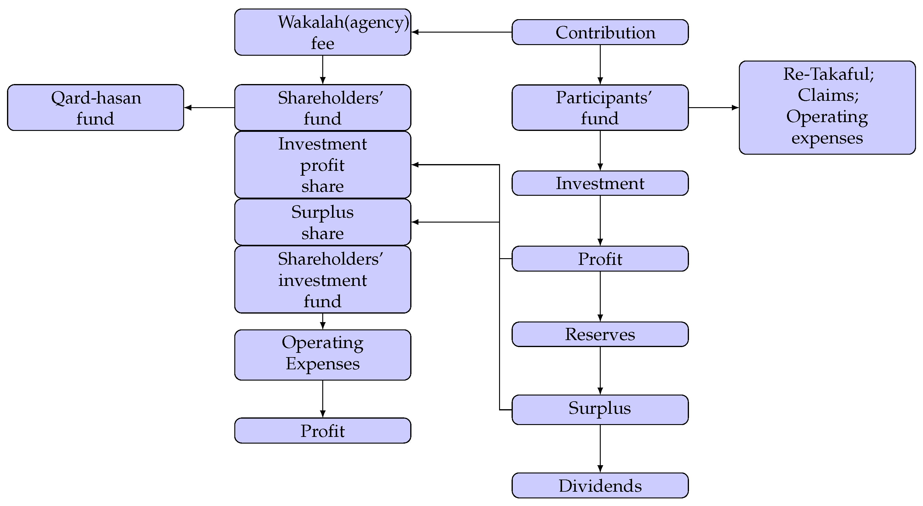
In regard to the underwriting activities, the Takaful operator acts as a Wakeel (agent) on behalf of participants to manage the Takaful fund. As shown in Figure 1, the operator manages the Takaful fund and pays all the incurred expenses to the participants. In exchange for these tasks, the company charges each participant a predefined fee known as a Wakalah fee. This fee is deducted initially and goes to the shareholders’ fund.

The Hybrid-Takaful model applies the Mudarabah contract (profit-sharing basis) for the investment activities. The operator manages the assets and shares the income generated from the investment based on a predetermined profit share ratio. In this contract, the operator, as a fund manager or mudarib, will receive profit depending on the performance of the investment.

The income generated from an investment, after the deduction by mudarib’s fee for the operator in conjunction with the underwriting surplus, represents the surplus in Takaful (participants’) fund. All the surplus account are property of the Takaful participants. However, a Takaful operator may receive an additional fee, in the form of incentive or performance fee, when the Takaful fund produces a surplus. This fee is determined as a percentage of the surplus generated in the Takaful fund. The remaining profit is then distributed to the participants.

When the Takaful fund experiences a deficit, there are two available options to consider. The first option is to charge the participants with additional contributions to cover the deficit value. However, this practice is not popular as it is not commercially feasible (Tolefat and Asutay 2013). The second option is the qard-hasan facility. This option is more popular in practice and it is not only encouraged by the Islamic Financial Shariah Board (IFSB 2010), but is also a mandatory requirement by some regulatory authorities. For this reason the proposed risk model focuses only on the qard-hasan option in addressing the issue arising from the deficit.

Qard-hasan, which is often called the benevolent loan, is an interest-free loan facility that is provided by shareholders as short term solvency resources to the participants’ fund in case of a deficit. Qard-hasan is a part of the shareholders’ capital that is specially earmarked to maintain the solvency of the participants’ fund. According to the IFSB (2010) regulation, any drawn down qard-hasan needs to be repaid out of future surpluses of the participants’ fund. In the event when the borrower is unable to settle the loan, the lender cannot force the borrower to make a repayment, and they must accept this transaction as a charitable act. Most Islamic scholars, including Onagun (2011), Yusof et al. (2011), Tolefat and Asutay (2013), and Rahim et al. (2017), agree with the IFSB (2010)’s rules in relation to the treatment of qard-hasan facility.

3. Surplus Process for Hybrid-Takaful with Investment and Qard-Hassan Facility

In this section, we propose a surplus model for Hybrid-Takaful with investment activities and qard-hasan (non-interest loan) facility. The model is motivated by Kim and Drekic (2016), who consider a discrete-time dependent Sparre Andersen risk model in the context of conventional insurance. The first difference between our approach and the one by Kim and Drekic (2016) is in the loan fund feature. In our model, there is no interest in undertaking loans, as in the conventional model. The second difference is in the loan repayment arrangement. While the borrower in Kim and Drekic (2016) is forced to pay the loan undertaking (including interest) when it exceeds a certain level (i.e., loan capacity), in our model the borrower will repay the loan only if they generate a positive surplus in the future. The assumption of the loan arrangement in our model consistent with the IFSB’s rule. However, the lenders have a right to get a part of each shared underwriting dividend to compensate for their effort to provide a benevolent loan. The third difference relates to the assumption that the undrawn-down loan can be invested. The undrawn-down loan is the loan facility that is still available in the loan fund. In case of Takaful the loan fund is the qard-hasan fund. We should note that Achlak (2016) has also developed a Takaful risk model based on Kim and Drekic (2016) but with the assumption that the loan facility does not need to be repaid and can not be invested. In our study, we assume that the loan facility (i.e., qard-hasan facility) will be repaid from the future surplus, and the undrawn-down qard-hasan facility will be invested to enhance the facility. Finally, our model provides the option to invest in a risk-free or risky asset, and takes into account Mudharabah or fund management fee for operator from each generating investment return. In our Hybrid-Takaful risk model, we incorporate the following four separate financial accounts:

• U: surplus fund
• $F^I$: investment fund
• $F^Q$: qard-hasan fund
• $F^L$: liability account

and three thresholds levels:

• $l^W$: the minimal requirement of Takaful surplus level
• $l^I$: trigger level for investment activities
• $l^D$: trigger level for dividend payment

where the levels are assumed to satisfy $0\le l^W\le l^I\le l^D$.

As explained in Section 2.2, there are two separate financial accounts in Takaful, namely participants’ funds and shareholders’ funds. The participants’ fund in our model is sub-divided into two separate financial accounts, namely, the surplus fund U and the investment fund $F^I$. The reason for the separation of the two accounts is for better financial management, while the underwriting activities are represented in the surplus fund U, the financial activities are in the investment fund $F^I$. The qard-hasan fund is a part of shareholders’ fund that is specially allocated as a benevolent loan for participants in case of deficit occurring due to underwriting activities. In our model, the drawn-down qard-hasan needs to be repaid from future surplus of the participants’ fund. We introduce the liability account $F^L$ to keep track of the total of qard-hasan borrowed and refunded. In our model we assume that all funds are in discrete monetary accounts. We adopt this assumption to facilitate the recursive calculation of finite-time ruin probability in Section 4.3.

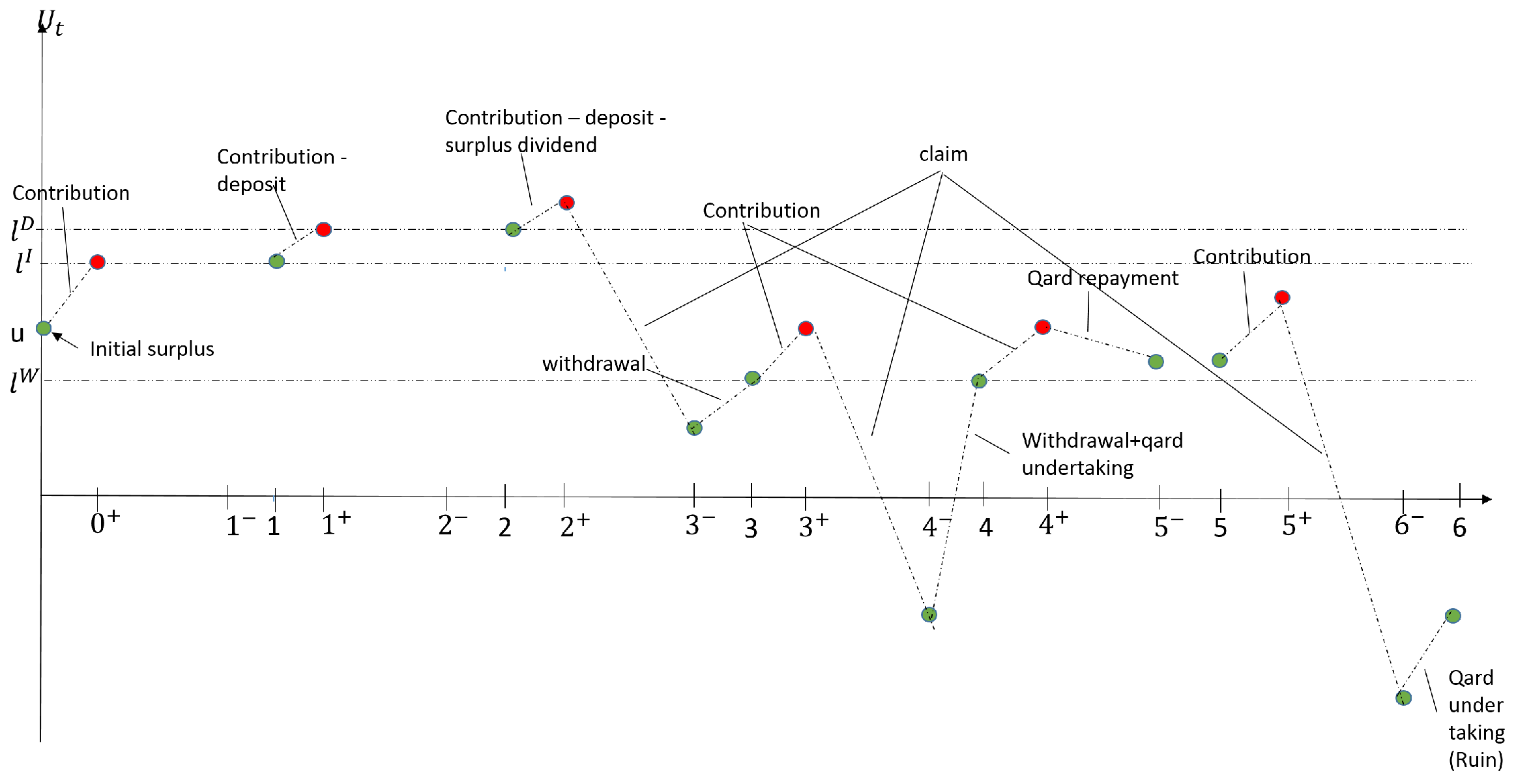
By $U_t,F_t^I,F_t^Q$, and $F_t^L$ we denote the values of surplus level, the investment fund, the qard-hasan fund, and the liability account, respectively, at the end of the time interval $(t-1,t],t\in {\mathbb{Z}}^{+}$ (where ${\mathbb{Z}}^{+}=\{1,2,\dots \}$). We assume that a constant contribution (premium) of $b\in {\mathbb{Z}}^{+}$ is received at $(t-1)+$, while claims are applied at $t-$. We also define $U_{t-},F_{t-}^I,F_{t-}^Q$, and $F_{t-}^L$ as the participants’ surplus fund, investment fund, qard-hasan facility, and liability, respectively, immediately after a claim instance but before a withdrawal, borrowing, qard-hasan undertaking, and qard-hasan repayment instance.

A dividend trigger level $l^D$ is a threshold that determines the dividend payment scenario. If $U_t\ge l^D$, a dividend amount of ${\delta }_t^i,i=\{1,2\}$ from the underwriting surplus will be shared among participants and shareholders. In our model, we propose two options for the dividend distribution. In the first one, denoted by ${\delta }_t^1$, we assume a constant dividend, while in the second, denoted by ${\delta }_t^2$, we use a similar assumption to that adopted by Achlak (2016), namely, that the dividend is equal to $U_t-l^D$. We assume that the percentage of the dividends distributed to the participants and to the shareholders are given by x and $1-x$, respectively, where $x\in (0,1)$.

We define $P_t$ as the contribution received at time t and $D_t^S$ as the total dividend distributed to shareholders at time t. Thus,

$$P_t=\left\{\begin{array}{cc}b,\hfill & \mathrm{if}{U}_t<l^D\hfill \\ b-x{\delta }_t^i,\hfill & \mathrm{if}{U}_t\ge l^D\hfill \end{array}\right.$$

(4)

$$D_t^S=\left\{\begin{array}{cc}0,\hfill & \mathrm{if}{U}_t<l^D\hfill \\ (1-x){\delta }_t^i,\hfill & \mathrm{if}{U}_t\ge l^D,\hfill \end{array}\right.$$

(5)

where ${\delta }_t^1=\delta \le b,\delta \in {\mathbb{Z}}^{+}$ and ${\delta }_t^2=U_t-l^D.$

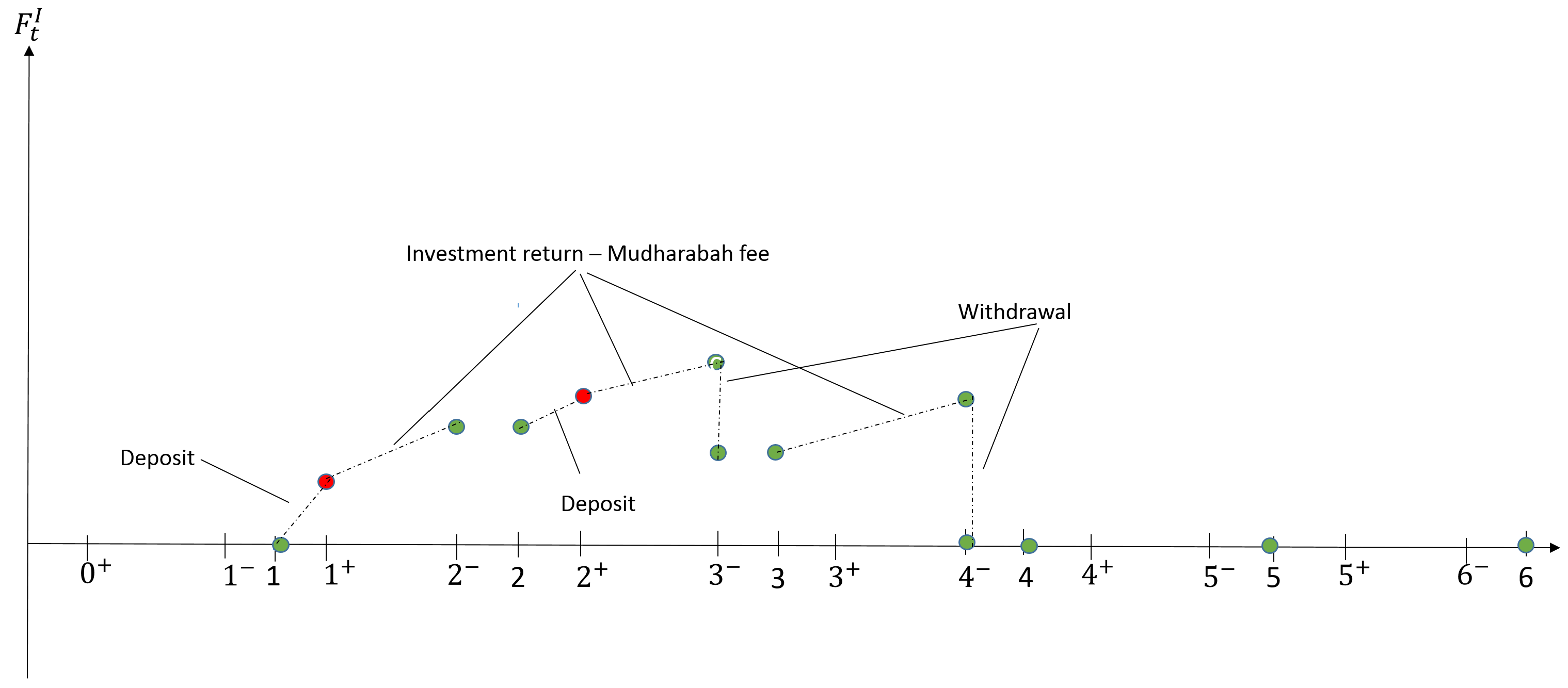
A threshold $l^I$ is a trigger point for investment activities. If $U_t\ge l^I$, a constant amount $d\in {\mathbb{Z}}^{+}$ is re-distributed to the investment fund at time $t+$. We assume that investment activities during each time interval are carried out after all of the outstanding debts and claims are paid out. We denote the deposit amount corresponding to the time interval $(t,t+1]$ as $D_t^I$, thus

$$D_t^I=\left\{\begin{array}{cc}0,\hfill & \mathrm{if}{U}_t<l^I\hfill \\ d,\hfill & \mathrm{if}{U}_t\ge l^I.\hfill \end{array}\right.$$

(6)

Note that from Equations (5) and (6), if $U_t>l^D$, then both $D_t^S$ and $D_t^I$ are paid.

We also assume that the operator, as a fund manager, may invest in the Shariah (permissible) non-risky or risky assets, like sukuk (Islamic bond) or a Shariah stock. In Takaful, the operator acts as a fund manager as well. Hence, they have the right to receive “salary” from the participants’ fund due to this role. A Hybrid-Takaful model applies Mudarabah (profit-sharing) for an investment activity in which the operator receives a dividend payment from investment generated profit. We assume that the fund manager receives $y\in (0,1)$ part of an investment gain.

Threshold $l^W$ represents the minimum level of the acceptable surplus of the participants’ fund. If $U_{t-}$ drops, at some time between $t-1$ and t, below $l^W$ due to claims, we withdraw from $F^I$, or borrow from $F^Q$, to bring the surplus fund up to level $l^W$ at time t. A withdrawal from the investment account $F^I$ is utilized first. We consider undertaking a interest-free loan from qard-hasan facility if the investment fund $F_{t-}^I$ is not sufficient to bring the surplus level back to $l^W$. The maximum qard-hasan that can be drawn down at time t is the maximum value of $F_t^Q$ or the remaining money needed by $U_t$ to reach $l^W$, whichever is smaller. The process will continue as long as the surplus-value is not negative. We assume that the un-drawn down qard-hasan fund will be invested in a risky or non-risky asset. The un-drawn down and investment gains will remain in the qard-hasan account to strengthen its facility. We denote the withdrawals and the qard-hasan undertaking amounts occurring during the time interval $(t-1,t]$ by $W_t^I$ and $W_t^Q$, respectively. The above descriptions imply the following formulae:

$$W_t^I=\left\{\begin{array}{cc}0,\hfill & \mathrm{if}{U}_{t-}\ge l^W\hfill \\ min\{F_{t-}^I,(l^W-U_{t-})\},\hfill & \mathrm{if}{U}_{t-}<l^W\hfill \end{array}\right.$$

(7)

$$W_t^Q=\left\{\begin{array}{cc}0,\hfill & \mathrm{if}{U}_{t-}\ge l^W\hfill \\ min\{F_{t-}^Q,max\{0,(l^W-U_{t-}-F_{t-}^I)\}\},\hfill & \mathrm{if}{U}_{t-}<l^W.\hfill \end{array}\right.$$

(8)

Participants need to repay their total qard-hasan undertaking to the qard-hasan fund $F^Q$ in the future period when their surplus value is greater than $l^W$. We assume that the loan repayment will be paid instantly after the claim is paid out at $t-$. If the surplus after claim payout at $t-$ is greater than $l^W$, then the loan will be repaid at $t-$. The loan repayment amount should not make the surplus-value drop below $l^W$ in any period. Unlike in the conventional counterpart, in the case when participants are not able to repay the qard-hasan, the undertaking qard-hasan will be counted as charity from shareholders to the participant. The participants are not obligated to repay the loan in case of a deficit. So, in our model, the loan repayment will not be the reason for ruin, but it will affect the value of $U_t$ and $F_t^Q$ instead. We define $D_t^Q$ as the qard-hasan repayment corresponding to the time interval $(t-1,t]$. Thus, we have

$$D_t^Q=\left\{\begin{array}{cc}0,\hfill & \mathrm{if}{U}_{t-}\le l^W\hfill \\ min\{F_{t-}^L,(U_{t-}-l^W)\},\hfill & \mathrm{if}{U}_{t-}>l^W.\hfill \end{array}\right.$$

(9)

Finally, the surplus level at time t is the initial level of u plus the total cash inflows from: contributions, withdrawal from investment fund, and loan undertaking from qard-hasan facility, minus the total cash outflows to: deposit investment, qard-hasan repayment, and claim payments. Thus,

$$U_t=u+\sum _{i=0}^{t-1}{P}_i-\sum _{i=0}^{t-1}{D}_i^S-\sum _{i=0}^{t-1}{D}_i^I-\sum _{i=1}^t{D}_i^Q+\sum _{i=1}^t{W}_i^I+\sum _{i=1}^t{W}_i^Q-\sum _{i=1}^{N_t}{X}_i.$$

(10)

We assume that the claim distribution of $N_t$ and $X_t$ has the same structure as in Sparre Andersen models Cheung et al. (2010). We also assume that the times between claims $(i-1)$ and i, $i\in {\mathbb{Z}}^{+}$, are described by independent and identically distributed (iid) positive random variables $\{W_i,i\in {\mathbb{Z}}^{+}\}$ with probability mass function (pmf) $a_k$ and the corresponding survival function $A_k$:

$$a_k=Pr\{W_i=k\},k=1,2,\dots ,n_a,$$

(11)

where $n_a\in {\mathbb{Z}}^{+}$ represents the upper bound for the interclaim times. Thus, for $k\le n_a$, we have

$$A_k=Pr\{W_i>k\}=1-\sum _{j=1}^k{a}_j.$$

(12)

We denote by ${\alpha }_j(k)$ the conditional pmf of $X_i$ given $W_i=k$:

$${\alpha }_j(k)=Pr\{X_i=j|W_i=k\},j\in {\mathbb{Z}}^{+},$$

(13)

and hence the joint pmf of $(W_i,X_i)$ is of the form

$$Pr\{W_i=k,X_i=j\}=a_k{\alpha }_j(k).$$

(14)

We also assume that the pairs $(W_i,X_i)$ are iid.

In order to visualize the cash flow in our proposed Takaful risk model, Figure 2, Figure 3, Figure 4 and Figure 5 present illustrative examples of the evolution of the surplus fund, investment fund, qard-hasan facility fund, and the liability level respectively. Appendix B summarizes the key symbols that are used in the paper. The surplus fund starts from an initial level u, and the maximum capacity of the qard-hasan facility that is provided by shareholders at the initial point is $f_Q$. The investment fund and the liability level are zero at the initial period. In each period, at time $(t-1)+$ there is contribution income deducted by deposit from investment fund and dividend payment if the corresponding trigger points are reached at time t. If surplus drops below the level $l^W$ due to claim payments at $t-$, we withdraw from the investment fund and/or qard-hasan facility. Every qard-hasan undertaking and repayment activities is recorded in the liability fund.

4. Finite-Time Ruin Probability for Hybrid-Takaful

This section describes a method of calculating a finite-time ruin probability associated with the Takaful risk model described by Equation (10). In particular, our goal is to derive the probability of ruin occurring before time $\tau <\infty$, which we denote by $\Psi (v,g_I,g_Q,g_L,\tau )$:

$$\Psi (v,g_I,g_Q,g_L,\tau )=Pr\{T\le \tau |U_0=v,F_0^I=g_I,F_0^Q=g_Q,F_0^L=g_L\},\tau \in {\mathbb{Z}}^{*},$$

(15)

where ${\mathbb{Z}}^{*}=\{0,1,2,..\}$ and T is defined in (1). In practice, $\tau$ represents the planning horizon of the insurance company. Typically, for non-life insurance, the managers set $\tau$ to four or five years (Burnecki et al. 2005).

To calculate the finite-time ruin probability, we follow Cossette et al. (2006) and Kim and Drekic (2016) by calculating the conditional survival probability of the first claim occurrence recursively. We define $\sigma (u,f_I,f_Q,f_L,n,m)$ as the finite-time survival probability until time n given that the initial level of surplus, investment fund, qard-hasan facility, and liability level are $u,f_I,f_Q$ and $f_L$ respectively, and the elapsed time $M_0$ since the most recent claim occurrence is m:

$$\sigma (u,f_I,f_Q,f_L,n,m)=Pr\{T>n|U_0=u,F_0^I=f_I,F_0^Q=f_Q,F_0^L=f_L,M_0=m\}.$$

(16)

Then, the finite-time ruin probability (15) can be represented as:

$$\Psi (v,g_I,g_Q,g_L,\tau )=1-\sigma (v,g_I,g_Q,g_L,\tau ,0).$$

(17)

In Section 4.3 we develop a recursive formula for the finite-time survival probability. For this, we construct some auxiliary variables, namely the maximum value of the fund processes in Section 4.1 and a calling point in Section 4.2.

4.1. The Maximum Value of Funds Process

The surplus fund in Equation (10) is a stochastic function whose value might be decreasing or increasing depending on the claim payments. In this section we construct a formula to calculate the maximum value of the surplus fund ${\widehat{U}}_{(t,u)}$, investment fund ${\widehat{F}}_{(t,u,f_I)}^I$, qard-hasan fund ${\widehat{F}}_{(t,f_Q)}^Q$, and liability level ${\widehat{F}}_{(t,f_L)}^L$ that represent levels of funds under the assumption of no claim, no withdrawal, no qard-hasan undertaking, and no qard-hasan repayment at time t given that the initial levels are $U_0=u,F_0^I=f_I,F_0^Q=f_Q,F_0^L=f_L$. Notice that ${\widehat{U}}_{(t,u)}$ and ${\widehat{F}}_{(t,f_L)}^L$ are non-decreasing functions of t, while ${\widehat{F}}_{(t,u,f_I)}^I$ and ${\widehat{F}}_{(t,f_Q)}^Q$ are non-decreasing functions of t if the investment returns are always positive. In our model, we use two different assumptions of investment returns, the first one is a constant positive rate of return, and the second one is a stochastic return. The first assumption is similar to the one adopted by Kim and Drekic (2016) and Achlak (2016).

To calculate the maximum value of surplus process ${\widehat{U}}_{(t,u)}$ and the maximum value of the investment return ${\widehat{F^I}}_{(t,u,f_I)}$, we need to identify the time points when the surplus level reaches the threshold levels $l^W$ and $l^I$ under the assumption of no claim, no withdrawal, and no qard-hasan undertaking and repayment. Under these assumptions, the surplus fund grows at a constant rate b (i.e., the contribution payment) from time 0 until the surplus level reaches the threshold level $l^I$. From the time point when the surplus level reaches $l^I$ until it reaches $l^D$, the surplus fund grows with a constant rate of $b-d$ due to the deposit payment to the investment fund. Denote by $z_{(u)}^I$ and $z_{(u)}^D$ the time points when the surplus level with the initial value u reaches the trigger points $l^I$ and $l^D$, respectively; i.e.,

$$z_{(u)}^I=\left\{\begin{array}{cc}0,\hfill & \mathrm{if}u\ge l^I\hfill \\ ⎡\frac{l^I-u}{b}⎤\hfill & \mathrm{if}u<l^I\hfill \end{array}\right.$$

(18)

and

$$z_{(u)}^D=\left\{\begin{array}{cc}0,\hfill & \mathrm{if}u\ge l^D\hfill \\ ⎡\frac{l^D-u-b{z}_{(u)}^I}{b-d}+z_{(u)}^I⎤\hfill & \mathrm{if}u<l^D,\hfill \end{array}\right.$$

(19)

where ⎡x⎤ represents the least integer greater than or equal to x.

4.1.1. The Maximum Value of Surplus Fund

Under the assumption of no claim, no withdrawal, no borrowing, and no loan repayment, the surplus process in Equation (10) becomes:

$${\widehat{U}}_{(t,u)}=u+\sum _{i=0}^{t-1}{P}_i-\sum _{i=0}^{t-1}{D}_i^S-\sum _{i=0}^{t-1}{D}_i^I.$$

(20)

By using the definition of premium $P_t$ (Equation (4)), dividend payout to shareholders $D_t^S$ (Equation (5)), deposit $D_t^I$ (Equation (6)), and the time points when the surplus level reaches the threshold level $l^W$ and $l^I$ (i.e., Equations (18) and (19)), it is easy to find the maximum value of the surplus fund ${\widehat{U}}_{(t,u)}$ as

$${\widehat{U}}_{(t,u)}=u+bt-d{(t-z_{(u)}^I)}_{+}-\delta {(t-z_{(u)}^D)}_{+},t\in {\mathbb{Z}}^{+},$$

(21)

when we consider a constant dividend ${\delta }_t^1=\delta \in {\mathbb{Z}}^{+}$, or

$${\widehat{U}}_{(t,u)}=\left\{\begin{array}{cc}u+bt-d{(t-z_{(u)}^I)}_{+}\hfill & \mathrm{if}t\le z_{(u)}^D\hfill \\ l^D+b-d\hfill & \mathrm{if}t>z_{(u)}^D,\hfill \end{array}\right.$$

(22)

when we consider dividend as ${\delta }_t^2=U_t-l^D$ with $x_{+}=max\{x,0\}$.

Equations (21) and (22) can be explained as the total cash inflow and outflow to the surplus fund. Before the time point $t=z_{(u)}^I$, there is only regular cash inflow, which is the constant contribution (tabaru) of b. Between $z_{(u)}^I$ and $z_{(u)}^D$, there is a regular outflow from the surplus process (${\widehat{U}}_{(t,u)}$) to the investment fund (${\widehat{F}}_{(t,u,f_I)}^I$), which is the deposit of d, in addition to the regular contribution payment. When the surplus reaches level $l^D$ at $z_{(u)}^D$, the dividend of ${\delta }_t^i,i=\{1,2\}$, will be distributed to the participants and shareholders. In addition to that, starting from $z_{(u)}^D$, the surplus fund ${\widehat{U}}_{(t,u)}$ will receive the contribution of b minus deposit d afterwards.

4.1.2. The Maximum Value of External Funds with Non-Risky Investment Return

In this section we assume that the operator, as a fund manager, invests the investment fund in the Shariah (permissible) non-risky asset like sukuk (Islamic bond) with a constant rate of return $k_1\ge 0$. We also assume that the un-drawn down qard-hasan fund will be invested at a constant investment gain of $k_2\ge 0$. The un-drawn down qard-hasan and those investment gains will remain in the qard-hasan fund to strengthen the qard-hasan facility. It is noted that there is no interest in the undertaking loan from the qard-hasan account.

The initial value of the investment fund ${\widehat{F}}_{(t,u,f_I)}^I$ will grow from its initial value $f_I$ at the rate of $k_1$ due to investment activities. In addition to this, the investment fund will be increased by deposit d, regularly from $z_{(u)}^I$ until time t. In each period, y percentage of the investment gain will be shared with the operator as the Mudharabah fee. Therefore, the non-recursive form of the investment fund is given by

$${\widehat{F}}_{(t,u,f_I)}^1=f_I{(1+k_1^{\prime })}^t+d_{z_{(u)}^I,t}^{k_1^{\prime }}$$

(23)

where ⎣x⎦ is a floor function representing the greatest integer less than or equal to x, and

$$k_1^{\prime }=(1-y)k_1$$

(24)

denotes the investment gain after deducting the Mudharabah fee. The total future value of deposits made at times $z_{(u)}^{I+}$ up to time $t-1$ with respect to the investment gain $k_1^{\prime }$ will be denoted by $d_{z_{(u)}^I,t}^{k_1^{\prime }}$:

$$d_{z_{(u)}^I,t}^{k_1^{\prime }}=d(1+k_1^{\prime })+d{(1+k_1^{\prime })}^2+\dots +d{(1+k_1^{\prime })}^{(t-z_{(u)}^I)}.$$

The sum on the right-hand side can be calculated explicitly as

$$d_{z_{(u)}^I,t}^{k_1^{\prime }}=\left\{\begin{array}{cc}0,\hfill & \mathrm{if}{z}_{(u)}^I>t\hfill \\ d(1+k_1^{\prime })\frac{{(1+k_1^{\prime })}^{t-z_{(u)}^I}-1}{k_1^{\prime }},\hfill & \mathrm{if}{z}_{(u)}^I\le t.\hfill \end{array}\right.$$

(25)

With the assumption of no qard-hasan undertaking and no qard-hasan repayment, there is no cash inflow or outflow except investment gains accumulated at the rate of $k_2$:

$${\widehat{F}}_{(t,f_Q)}^Q=⎣f_Q{(1+k_2)}^t⎦.$$

(26)

The investment fund and qard-hasan fund may take non-integer values due to interest accumulation. However, we apply the floor function in the Equations (23) and (26) to round down the value as we assume that all funds are in the discrete monetary units. Taking the lower bound value of the investment and qard-hasan funds can be seen as conservative.

The liability level under the assumption of no loan undertaking and repayment will remain the same as the initial liability level:

$${\widehat{F}}_{(t,f_L)}^L=f_L$$

(27)

for $t\in {\mathbb{Z}}^{*}.$

4.1.3. The Maximum Values of External Funds with Risky Investment Return

In this section we assume that the investment returns are not constant. The Takaful operator invests the funds (investment and qard-hasan) in the same risky asset, for example, in the Shariah compliant stock or floating Sukuk (Islamic bond). In our study, we model the asset price in discrete time by a Markov chain that satisfies the recursive form $S_{n+1}=S_n{Y}_{n+1}$, where $\{Y_i\}$ are iid random variables. If the initial price is $S_0$, then expanding the recursion yields

$$S_n=S_0\prod _{i=1}^n{Y}_i.$$

(28)

Therefore, the maximum value of qard-hasan facility (${\widehat{F^Q}}_{(t,f_Q)}$) with the initial value $f_Q$ is:

$${\widehat{F}}_{(f_Q,t)}^Q=f_Q\prod _{i=1}^t{Y}_i.$$

(29)

To calculate the maximum value of the investment fund (${\widehat{F^I}}_{(t,u,f_I)}$), we need to add the deposits and share the y part of Mudharabah fee. If the investment generates a positive return, then we need to share y part of the return with Takaful operator. Notice that the rate of return in the market model (28) is $\frac{S_i-S_{i-1}}{S_{i-1}}=Y_i-1$. Then the real rate of return on the investment fund is: $(1-y)(Y_i-1)=(Y_i-y{Y}_i+y)-1=Y_i^{*}-1$, where we assume that $Y_i>1$. Thus, the rate of return is $Y^{*}-1$ with $Y^{*}$ defined as:

$$Y_i^{*}=\left\{\begin{array}{cc}{Y}_i,\hfill & \mathrm{if}{Y}_i\le 1,\hfill \\ Y_i-y{Y}_i+y,\hfill & \mathrm{if}{Y}_i>1.\hfill \end{array}\right.$$

(30)

Therefore, the maximum value of the investment fund (${\widehat{F^I}}_{(t,u,f_I)}$) with initial value $f_I$ and deposit d is

$${\widehat{F^I}}_{(t,u,f_I)}=f_I\prod _{i=1}^t{Y}_i^{*}+\sum _{i=z_{(u)}^I}^{t-1}d\prod _{j=i+1}^t{Y}_i^{*}.$$

(31)

If we assume that $\{Y_i\}$ has a distribution $P(Y=j^u)=p$, $P(Y=j^d)=1-p$, then the asset price at $n+1$, given the value of $S_n$, is

$$S_{n+1}|S_n=\left\{\begin{array}{cc}{j}^u{S}_n,\hfill & \mathrm{with}\mathrm{probability}p,\hfill \\ j^d{S}_n,\hfill & \mathrm{with}\mathrm{probability}1-p.\hfill \end{array}\right.$$

Under this model, in each time period, the asset price will go up by a constant factor of $j^u$ with probability p, or go down by a constant factor of $j^d$ with probability $1-p$, with $j^u\ge 1\ge j^d\ge 0$. At the time n, there are $2^n$ possible state prices. This model is known in mathematical finance as a binomial market model. In insurance, binomial models have been applied to the problem of pricing of equity linked products (see, for example, Costabile 2018; Costabile et al. 2008).

Under the assumption of the binomial price model, we can calculate the maximum values of the external funds via the following algorithms. We define the maximum value of the investment fund at time t for state price l as

$${\widehat{F}}_{(t,u,f1,l)}^I=⎣F_I(t,u,f_I,l)⎦,l=1,\dots ,2^t,$$

(32)

where $F_I(t,u,f_I,l)$ can be calculated recursively by

$$F_I(t,u,f_I,l)=\left\{\begin{array}{cc}{f}_I,\hfill & \mathrm{if}t=0,\hfill \\ F_I(t-1,u,f_I,⎡l/2⎤)(j^u-y{j}^u+y),\hfill & \mathrm{if}0<t\le z_{(u)}^I,l=\{1,3,5,..,N_l(t)-1\},\hfill \\ F_I(t-1,u,f_I,l/2)j^d,\hfill & \mathrm{if}0<t\le z_{(u)}^I,l=\{2,4,6,..,N_l(t)\},\hfill \\ (F_I(t-1,u,f_I,⎡l/2⎤)+d)(j^u-y{j}^u+y),\hfill & \mathrm{if}t>z_{(u)}^I,l=\{1,3,5,..,N_l(t)-1\},\hfill \\ (F_I(t-1,u,f_I,l/2)+d)j^d,\hfill & \mathrm{if}t>z_{(u)}^I,l=\{2,4,6,..,N_l(t)\}\hfill \end{array}\right.$$

(33)

with $N_l(t)$ representing the number of state price at time t. Before the surplus reaches the dividend trigger level $l^I$ at $z_{(u)}^I$, the investment fund grows at a rate of return of $Y^{*}-1$ (see Equation (30)). Starting from $z_{(u)}^I$, the investment fund receives a deposit d from the surplus fund, and it is also invested at the same rate of return $Y^{*}$. The state price $l\in \{1,3,5,..,N_l(t)-1\}$ represents the upward movements, while the state price $l\in \{2,4,6,..,N_l(t)\}$ represents the downward movements.

The maximum value of qard-hasan fund at time t for state price l as

$$F_{(t,f_Q,l)}^Q=⎣F_Q(t,f_Q,l)⎦,l=1,..,N_l(t),$$

(34)

where $f_Q(t,f_Q,l])$ can be calculated recursively by

$$F_Q(t,f_Q,l)=\left\{\begin{array}{cc}{f}_Q,\hfill & \mathrm{if}t=0,\hfill \\ F_Q(t-1,f_Q,⎡l/2⎤)j^u,\hfill & \mathrm{if}t>0,l=\{1,3,5,..,N_l(t)-1\},\hfill \\ F_Q(t-1,f_Q,l/2)j^d,\hfill & \mathrm{if}t>0,l=\{2,4,6,..,N_l(t)\}.\hfill \end{array}\right.$$

(35)

The investment fund grows at a rate of return $Y-1$ with a constant upward magnitude $j^u$ and downward magnitude $j^d$.

If by $P(t,l)$ we denote the probability of the state price l at time t, then these probabilities can be calculated recursively by

$$P(t,l)=\left\{\begin{array}{cc}1,\hfill & \mathrm{if}t=0,\hfill \\ P(t-1,⎡l/2⎤)p,\hfill & \mathrm{if}t>0,l=\{1,3,5,..,N_l(t)-1\},\hfill \\ P(t-1,l/2)(1-p),\hfill & \mathrm{if}t>0,l=\{2,4,6,..,N_l(t)\}.\hfill \end{array}\right.$$

(36)

In each time period, the probability that the asset price will go up is p, while the probability that the asset will go down is $1-p$.

One example of the most popular binomial market model is the one by Cox et al. (1979). In this model, the magnitude of the upward jump is $j^u=e^{\sqrt{{\sigma }^2}}$, while the magnitude of the downward jump is $j^d=1/j^u$, and the probability of jump-up under the risk-neutral probability measure is $p=\frac{1+r-j^d}{j^u-j^d}$, where ${\sigma }^2$ is the asset’s variance and r is a fixed risk-free return.

4.2. Calling Point

In this subsection we define a calling point, denoted by $c_{(t,m,u,f_L)}$, which represents the earliest time point before time t when the debt from qard-hasan facility needs to be repaid before the first claim occurs. If the elapsed waiting time at time 0 since the most recent claim occurrence is m, and the upper bound for the the interclaim times is $n_a$ (see Equation (11)), then the next claim will occur before time $n_a-m$. Therefore the calling point $c_{(t,m,u,f_L)}$ is bounded by $min\{n_a-m,t\}$. Qard-hasan repayment will be paid if participants have positive liability, and the surplus fund is greater than $l^W$. Note that the surplus and the liability at time t under the assumption of no claim occurrence are ${\widehat{U}}_{(t,u)}$ and ${\widehat{F}}_{(t,f_L)}^L$, respectively. Then

$$c_{t,m,u,f_L}=\left\{\begin{array}{c}min\{n_a-m,t\},\mathrm{if}({\widehat{U}}_{(i,u)}\le l^W\mathrm{or}{\widehat{F}}_{(i,f_L)}^L<0)\forall i\in \{1,2,...,min\{n_a-m,t\}\}\hfill \\ min\{i\in \{1,2,...,min\{n_a-m,t\}\}|{\widehat{U}}_{(i,u)}>l^W\},\mathrm{otherwise}.\hfill \end{array}\right.$$

(37)

In Equation (37), the earliest time point to make a loan repayment is the earliest time the liability level ${\widehat{F}}_{(i,f_L)}^L$ becomes positive and the surplus value ${\widehat{U}}_{(i,u)}$ is greater than $l^W$, for $i=1,2...,min\{n_a-m,t\}$.

4.3. Recursive Formula to Calculate the Finite-Time Survival Probability

The aim of this subsection is to develop an algorithm to calculate the finite-time survival probability (16). Once we find this value, our goal of finding the ruin probability can be achieved by using (17). Under the condition of no external funds scenario, Cossette et al. (2006) propose a recursive algorithm to calculate the finite time survival probabilities as the sum of conditional finite time survival probabilities of the first claim occurring. Let us denote by ${\sigma }^C(u,n)$ and ${\sigma }^C(u,n,k)$, respectively, the finite-time survival probability and the finite time conditional survival probability given that the first claim occurs at time k, with the absence of external funds (i.e., $F_t^I=F_t^Q=F_t^L=0$). Then

$${\sigma }^C(u,n)=\sum _{k=1}^{n_a}{a}_k{\sigma }^C(u,n,k)=\sum _{k=1}^n{a}_k{\sigma }^C(u,n,k)+\sum _{k=n+1}^{n_a}{a}_k.$$

(38)

We should note that ${\sigma }^C(u,n,k)$ in Equation (38) is equal to 1 for $k>n$, because the claim occurrence after time n implies that the process survives until n. Under the absence of investment activity ($d=0$) and no dividend payment (${\delta }_t^i=0$), Cossette et al. (2006) define ${\sigma }^C(u,n,k),k\in \{1,2,..,n\}$ as the accumulation of weighted sum of ${\sigma }^C(u+bk-j,n-k)$, which is the probability of surviving the time interval $(k,n]$ with the level of surplus fund at time k after the claim payment is $u+bk-j$, for all possible values of claim severity j that do not cause ruin at time k. Then we have

$${\sigma }^C(u,n)={\displaystyle \sum _{k=1}^n}{a}_k{\displaystyle \sum _{j=1}^{u+bk}}{\alpha }_j(k){\sigma }^C(u+bk-j,n-k)+A_k.$$

(39)

By following the idea of Kim and Drekic (2016) of expanding the recursive Formula (39) with the existence of external funds, the finite time survival probability (16) can be found using the recursive algorithm as shown in Theorem 1.

Theorem 1.

Let $\sigma (u,f_I,f_Q,f_L,n,m)$ be the finite time survival probability at time n, with the initial values of the surplus fund, investment fund, qard-hasan fund, and liability level are equal to $u,f_I,f_Q$ and $f_L$, respectively, and the elapsed time at time 0 since the most recent claim occurrence is equal to m as defined in Equation (16). Then $\sigma (u,f_I,f_Q,f_L,n,m)$ can be calculated recursively via

$$\begin{array}{c}\sigma (u,f_I,f_Q,f_L,n,m)\hfill \\ \hfill ={\displaystyle \sum _{k=1}^{c_{(n,m,u,f_L)}}}\frac{a_{k+m}}{A_m}{\displaystyle \sum _{l=1}^{N_l(k)}}P(k,l){\displaystyle \sum _{j=1}^{{\widehat{U}}_{(k,u)}+{\widehat{F}}_{(k,u,f_I,l)}^I+{\widehat{F}}_{(k,f_Q,l)}^Q}}{\alpha }_j(k+m)\sigma (u^{*}(l),f_I^{*}(l),f_Q^{*}(l),f_L^{*}(l),n-k,0)\\ \hfill +\frac{A_{c_{(n,m,u,f_L)}+m}}{A_m}{\displaystyle \sum _{l=1}^{N_l(c_{(n,m,u,f_L)})}}P(c_{(n,m,u,f_L)},l)\sigma (u^{\prime },f_I^{\prime }(l),f_Q^{\prime }(l),f_L^{\prime },n-c_{(n,m,u,f_L)},c_{(n,m,u,f_L)}+m),\end{array}$$

(40)

with the boundary condition

$$\sigma (u,f_I,f_Q,f_L,n,m)=\left\{\begin{array}{cc}0,\hfill & ifu\in {\mathbb{Z}}^{-}\mathrm{or}m=n_a,\hfill \\ 1,\hfill & ifu\in {\mathbb{Z}}^{*},n=0,andm=0,1,...,n_a-1,\hfill \end{array}\right.$$

(41)

where $u^{*}(l),f_I^{*}(l),f_Q^{*}(l),f_L^{*}(l)$ are described in Theorem 2 below, while $u^{\prime },f_I^{\prime }(l),f_Q^{\prime }(l),f_L^{\prime }$ are described in Theorem 3. In the case of investment in a non-risky asset, we set $N_l(k)=1$, $P(k,l)=1$, ${\widehat{F}}_{(k,u,f_I,l)}^I={\widehat{F}}_{k,u,f_I}^I$ in Equation (23), and ${\widehat{F}}_{(k,f_Q,l)}^Q={\widehat{F}}_{k,f_Q}^Q$ in Equation (26).

Theorem 2.

The values $u^{*}(l),f_I^{*}(l),f_Q^{*}(l)$, and $f_L^{*}(l)$ in Equation (40) can be calculated using the following equations:

$$u^{*}(l)=min\{max\{{\widehat{U}}_{(k,u)}-j-{\widehat{F}}_{(k,f_L)}^L,l^W\},{\widehat{U}}_{(k,u)}-j+{\widehat{F}}_{(k,u,f_I,l)}^I+{\widehat{F}}_{(k,f_Q,l)}^Q\},$$

(42)

$$f_I^{*}(l)=min\{max\{{\widehat{F}}_{(k,u,f_I,l)}^I-l^W+{\widehat{U}}_{(k,u)}-j,0\},{\widehat{F}}_{(k,u,f_I,l)}^I\},$$

(43)

$$\begin{array}{c}\hfill f_Q^{*}(l)=min\{max\{min\{{\widehat{F}}_{(k,f_Q,l)}^Q+{\widehat{F}}_{(k,f_L)}^L,{\widehat{F}}_{(k,f_Q,l)}^Q+{\widehat{U}}_{(k,u)}-j-l^W\},{\widehat{F}}_{(k,f_Q,l)}^Q\},\\ \hfill max\{{\widehat{F}}_{(k,f_Q,l)}^Q+{\widehat{U}}_{(k,u)}-j-l^W+{\widehat{F}}_{(k,u,f_I,l)}^I,0\}\}\end{array}$$

(44)

$$\begin{array}{c}\hfill f_L^{*}=max\{min\{max\{0,{\widehat{F}}_{(k,f_L)}^L-{\widehat{U}}_{(k,u)}+j+l^W\},{\widehat{F}}_{(k,f_L)}^L\},\\ \hfill min\{{\widehat{F}}_{(k,f_L)}^L+{\widehat{F}}_{(k,f_Q,l)}^Q,{\widehat{F}}_{(k,f_L)}^L+l^W-{\widehat{U}}_{(k,u)}+j-{\widehat{F}}_{(k,u,f_I,l)}^I\}\}.\end{array}$$

(45)

Theorem 3.

The values $u^{\prime },f_I^{\prime }(l),f_Q^{\prime }$(l), and $f_L^{\prime }(l)$ in Equation (40) can be calculated using the following equations:

$$u^{\prime }={\widehat{U}}_{(c_{(n,m,u,f_L)},u)}-min\{{({\widehat{U}}_{(c_{(n,m,u,f_L)},u)}-l^W)}_{+},{\widehat{F}}_{(c_{(n,m,u,f_L)},f_L)}^L\},$$

(46)

$$f_I^{\prime }(l)={\widehat{F}}_{(c_{(n,m,u,f_L)},u,f_I,l)}^I,$$

(47)

$$f_Q^{\prime }(l)={\widehat{F}}_{(c_{(n,m,u,f_L)},f_Q,l)}^Q+min\{{({\widehat{U}}_{(c_{(n,m,u,f_L)},u)}-l^W)}_{+},{\widehat{F}}_{(c_{(n,m,u,f_L)},f_L)}^L\},$$

(48)

$$f_L^{\prime }={\widehat{F}}_{(c_{(n,m,u,f_L)},f_L)}^L-min\{{({\widehat{U}}_{(c_{(n,m,u,f_L)},u)}-l^W)}_{+},{\widehat{F}}_{(c_{(n,m,u,f_L)},f_L)}^L\}.$$

(49)

5. Numerical Results

In this section, we implement the algorithm from Section 4 to calculate the finite-time ruin probabilities based on the proposed Hybrid-Takaful model (i.e., Equation (17)) through recursive Formula (40). The objective is to study the effect some of the parameters may have on ruin probability and to investigate the performance of the proposed Takaful model in comparison with the conventional one. We use Wolfram-Mathematica version 9.0 to do all numerical calculations.

In our simulation study, we apply the set of input parameters as in Kim and Drekic (2016) and Achlak (2016), which will facilitate comparisons between the existing models and the proposed one. We assume that the interclaim time follows a truncated geometric distribution with $n_a=25$:

$$a_k=\left\{\begin{array}{cc}(2/11){(9/11)}^{(}k-1)\hfill & \mathrm{if}k=1,2,\dots ,24,\hfill \\ {(9/11)}^{24}\hfill & \mathrm{if}k=25,\hfill \end{array}\right.$$

while the claim size distribution follows a discretized version of the Pareto distribution with mean 10.5 and variance 120

$${\alpha }_j(k)={\alpha }_j={(1+\frac{j-1}{30})}^{-4}-{(1+\frac{j}{30})}^{-4},j\in {\mathbb{Z}}^{+}.$$

(50)

In all simulations, we set the contribution $b=5$, the initial value for the participants’ fund $v=10$, the initial value of the investment fund $g_I=0$, and the initial value of liability $g_L=0$. All these values are in the currency unit, for example, in million of dollars. We also assume that the rate of return for the investment fund ($k_1$) is 1% per month.

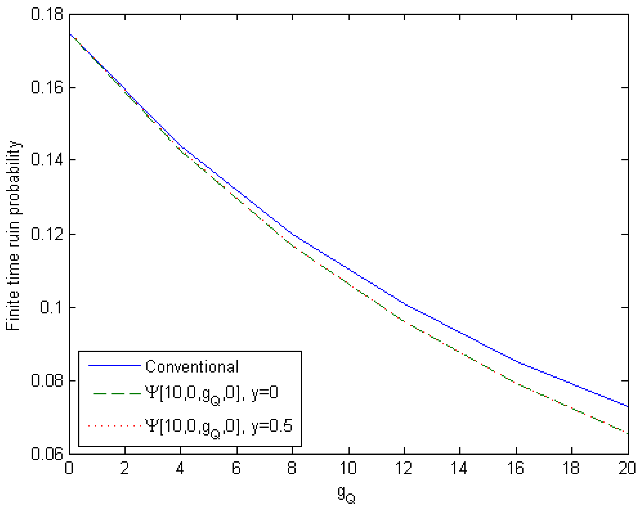
Figure 6 shows ruin probabilities for the time horizon $\tau =25$, and trigger points $l^W=0,l^I=20$, and $l^D=50$. We assume a constant dividend ${\delta }_t^1=\delta =3$, a deposit $d=1$, and an investment rate of return for qard-hasan fund $k_2=0.02$. We calculate ruin time probabilities for several values of the maximum loan capacity $g_Q$. In our Takaful model, we need the percentage of Mudharabah fee (y), while in the conventional model, this fee is zero. We consider two different values of y, namely 0 and 50%.

For the surplus and investment fund, our proposed model has similar features as the conventional counterpart by Kim and Drekic (2016). Hence, under the assumption of no loan facility and no Mudharabah fee, $g_Q=0$ and $y=0$, the ruin probabilities of our proposed Takaful model are the same as in the the conventional one. The difference between our model and Kim and Drekic (2016) model is in the features of the loan activities. In the conventional model, there is an interest rate charged in each loan. In addition to that, the borrower is forced to repay the loan if the loan undertaking (including the interest rate) exceeds the maximum loan capacity. This rule may increase the chance of a ruin occurring. The qard-hasan facility in our proposed Takaful model has two benefits; the loan capacity may positively grow as a result of investing the undrawn-down qard-hasan, and the loan will be repaid if there is enough money in the surplus fund. We may see from Figure 6 that the ruin probabilities of our proposed Takaful model with Mudharabah fee $y=0$ or $y=0.5$ are lower than the conventional counterpart. Moreover, a higher loan capacity produces a greater difference in ruin probabilities between the proposed Takaful model and the conventional one. The two different values of the Mudharabah fee that we have chosen in our implementation do not produce significantly different ruin probabilities.

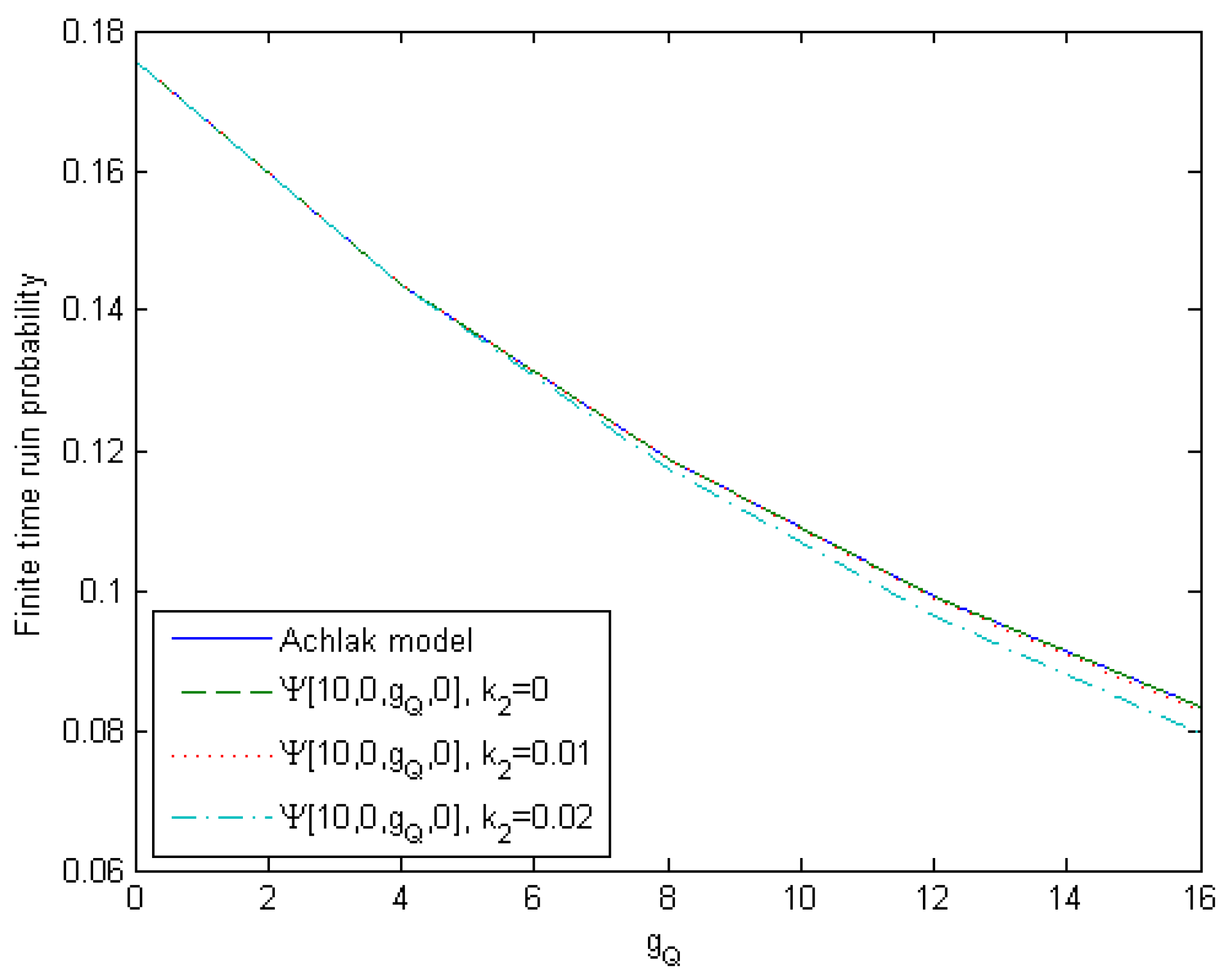
Figure 7 compares the Takaful ruin time probabilities based on the proposed model with probabilities based on the model proposed by Achlak (2016). In the Achlak (2016) model, the qard-hasan fund is not invested, and there is no obligation for the participants to return the qard-hasan undertaking. We apply the same dividend value ${\delta }_t^2=U_t-l^D$ as in Achlak (2016), with several values of the initial qard-hasan fund, $g_Q$. Other input parameters are the same as the input parameters that we use in the previous simulation.

We also set 3 different values of the rate of return for qard-hasan fund ($k_2\in \{0,0.01,0.02\}$). In the case of no qard-hasan facility, we obtain the same ruin probabilities as that based on the Achlak (2016) model for all values of $k_2$. This is because the surplus and investment features in our proposed model are the same as the ones in Achlak (2016). For $g_Q>0$, when the qard-hasan fund is not invested ($k_2=0$), the qard-hasan repayment in our proposed model causes the ruin probability to be slightly higher than the one without loan repayment. This result can be explained by the fact that loan repayment causes a delay in depositing the investment fund. However, if we invest in the qard-hasan fund, the obligation of loan repayment leads to lower ruin probabilities than those without loan repayment. The difference between finite-time ruin probabilities with and without loan repayment becomes more visible when the initial value of the qard-hasan fund ($g_Q$) increases.

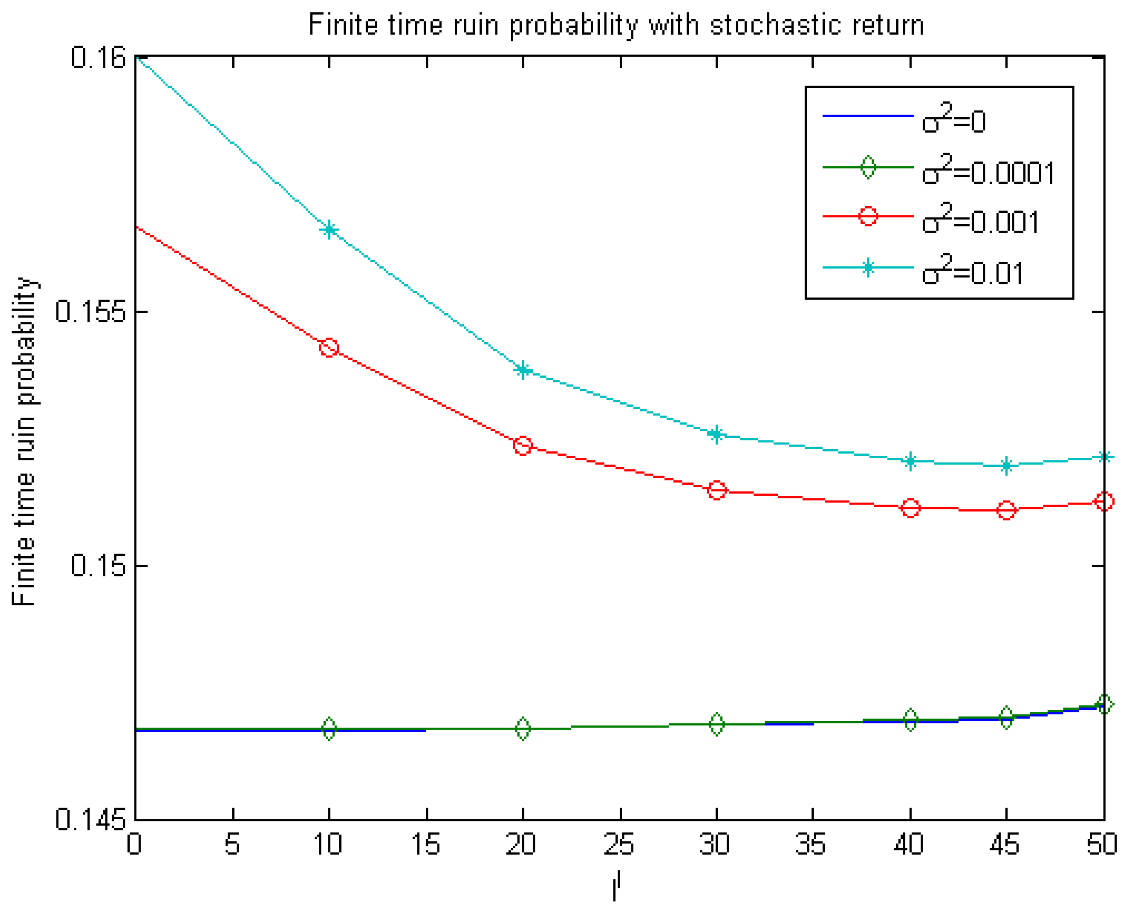
Figure 8 represents finite-time ruin probabilities for the time horizon $\tau =12$ with trigger points $l^W=0$, $0\le l^I\le 50$, $l^D=50$, initial qard-hasan fund $g_Q=10$, Mudharabah fee $y=5\%$, deposit $d=1$, and dividend $\delta =3$. We consider four different assumptions about the asset’s return: the first one is a non-risky asset with the rate of return of $1\%$ per month. The other three are risky assets with the expected rate of return of $1\%$ per month and variances 0.0001, 0.001, and 0.01. In this study we apply the Cox et al. (1979) model as explained in Section 4.1.3. The graph suggests that the finite-time ruin probabilities increase as the variance of the asset is increased. In addition, we may see that the finite-time ruin probabilities for non-risky assets (${\sigma }^2=0$) and risky assets with low variance (${\sigma }^2=0.0001$) increase as we increase the investment trigger level $l^I$. This phenomenon can be explained by the fact that when $l^I$ increases then deposits in investment activities will be delayed. This, in turn, reduces the probability of ruin, since positive returns are earned from investment activities on the external fund only. However, the previous argument does not apply to the case of investing in the risky asset with high volatility, which can be explained by the fact that investing in such assets may produce large negative returns that will reduce the total reserve of Takaful fund. Thus, higher volatility of the asset price will increase the riskiness of the Takaful product, in the sense that higher volatility of the asset’s return produces a higher ruin probability. For both ${\sigma }^2=0.001$ and $0.01$, the optimal level to invest is $l^I=45$ based on the ruin probability criterion.

6. Conclusions

In this paper, we propose a framework of Hybrid-Takaful that incorporates investment activities and qard-hasan facility. Qard-hasan (benevolent loan) facility is the non-interest loan provided by shareholders to Takaful participants in the case of a deficit. We assume that the qard-hasan undertaking will be returned if the participants’ fund gains surplus in the future. We construct a surplus process of the participants’ fund, and then derive a method of calculating finite-time ruin probabilities.

Based on our numerical simulations, we find that the qard-hasan facility improves the performance of the fund as it decreases the finite-time ruin probabilities. This can be explained by the fact that this facility, unlike in the conventional insurance, provides loans at no cost and no mandatory repayment when there is a deficit. In addition, paying off the qard-hasan undertaking not only follows the Shariah rule but also has a positive effect on the business, if we invest the undrawn-down qard-hasan in non-risky assets. By paying off the loan undertaking to the qard-hasan fund, we can guarantee that the fund will grow at the corresponding rate of return. If the fund remains in the surplus account, then the investment return is delayed until the surplus account reaches the investment trigger level.

Our study incorporates the option to invest the investment fund and qard-hasan fund in the same risky asset under the assumption of binomial CRR market model. For future research, we will extend the model to two correlated risky assets for the investment fund and qard-hasan fund. For this case, we may follow the idea of Moon et al. (2008), who constructed the binomial state price for two dependent assets.

References

1. Achlak, Arham. 2016. Discrete-Time Surplus Process for Takaful Insurance with Multipe Threshold Levels. Master’s dissertation, Middle East Technical University, Ankara, Turkey. [Google Scholar]
2. Al Rahahleh, Naseem, M. Ishaq Bhatti, and Faridah Najuna Misman. 2019. Developments in Risk Management in Islamic Finance: A Review. Journal of Risk and Financial Management 12: 37. [Google Scholar] [CrossRef] [Green Version]
3. Bappenas. 2018. The Indonesia Masterplan of Sharia Economy 2019–2024. Jakarta: Deputy of Economy Indonesian Ministry of National Development Planning. [Google Scholar]
4. Bhatti, Maria. 2019. Islamic dispute resolution in the United Kingdom. In Dispute Resolution in Islamic Finance: Alternatives to Litigation? Edited by Adnan Trakic, John Benson and Peraviz K. Ahmed. London: Routledge, chp. 4. pp. 54–67. [Google Scholar]
5. Bhatti, Maria. 2020. Managing Shariah Non-Compliance Risk via Islamic Dispute Resolution. Journal of Risk and Financial Management 13: 2. [Google Scholar] [CrossRef] [Green Version]
6. Bulinskaya, Ekaterina. 2017. New Research Directions in Modern Actuarial Sciences. In International Conference on Modern Problems of Stochastic Analysis and Statistics. Cham: Springer, vol. 208, pp. 349–408. [Google Scholar] [CrossRef]
7. Burnecki, Krzysztof, Paweł Miśta, and Aleksander Weron. 2005. Ruin probabilities in finite and infinite time. In Statistical Tools for Finance and Insurance. Edited by Pavel Cizek, Härdle Wolfgang Karl and Weron Rafał. New York: Springer, chp. 15. pp. 341–74. [Google Scholar]
8. Cheung, Eric CK, David Landriault, Gordon E. Willmot, and Jae-Kyung Woo. 2010. Structural properties of Gerber-Shiu functions in dependent Sparre Andersen models. Insurance: Mathematics and Economics 46: 117–26. [Google Scholar] [CrossRef]
9. Cossette, Helene, David Landriault, and Etienne Marceau. 2006. Ruin probabilities in the discrete time renewal risk model. Insurance: Mathematics and Economics 38: 309–23. [Google Scholar] [CrossRef]
10. Costabile, Massimo. 2018. Computing risk measures of life insurance policies through the Cox Ross Rubinstein model. The Journal of Derivatives 26: 86–94. [Google Scholar] [CrossRef]
11. Costabile, Massimo, Ivar Massabó, and Emilio Russo. 2008. A binomial model for valuing equity-linked policies embedding surrender options. Insurance: Mathematics and Economics 42: 873–86. [Google Scholar] [CrossRef]
12. Cox, John C., Stephen A. Ross, and Mark Rubinstein. 1979. Option pricing: A simplified approach. Journal of Financial Economics 7: 229–63. [Google Scholar] [CrossRef]
13. GIFR. 2019. Global Islamic Finance Report. Technical Report. Cambridge: Cambridge Institute of Islamic Finance. [Google Scholar]
14. Hassan, Kabir, and Michael Mahlknecht. 2011. Islamic Capital Markets: Products and Strategies. West Sussex: John Wiley and Sons. [Google Scholar]
15. Hussain, Mher Mushtaq, and Ahmad Tisman Pasha. 2011. Conceptual and Operational Diferences between General Takaful and Conventional Insurance. Australian Journal of Business and Management Research 1: 23–28. [Google Scholar]
16. IFDR. 2018. Islamic Finance Development Report: Building Momentum. Thomson Reuters. Available online: https://ceif.iba.edu.pk/pdf/Reuters-Islamic-finance-development-report2018.pdf (accessed on 11 January 2020).
17. IFSB. 2010. Islamic Financial Services Board Standard on Solvency Requirements for Takaful (Islamic Insurance) Undertakings. Kuala Lumpur: IFSB Publication. [Google Scholar]
18. Kassim, Zainal Abidin Mohd, Hassan Scott Odierno, and Sabbir Patel. 2013. Hybrid insurance structures: Reciprocals, hybrid mutual insurers, and takaful. In Takaful and Mutual Insurance: Alternative Approaches to Managing Risks. Edited by Serap O. Gönülal. Washingtonm: The World Bank, chp. 5. pp. 67–81. [Google Scholar]
19. Khan, Hayat. 2015. Optimal incentives for takaful (Islamic insurance) operators. Journal of Economic Behavior & Organization 109: 135–44. [Google Scholar] [CrossRef]
20. Khan, Hayat. 2019. A Nontechnical Guide on Optimal Incentives for Islamic Insurance Operators. Journal of Risk and Financial Management 12: 127. [Google Scholar] [CrossRef] [Green Version]
21. Kim, Sung Soo, and Steve Drekic. 2016. Ruin Analysis of a Discrete-Time Dependent Sparre Andersen Model with External Financial Activities and Randomized Dividends. Risks 4: 2. [Google Scholar] [CrossRef] [Green Version]
22. Loisel, Stéphane, and Hans-U. Gerber. 2012. Why ruin theory should be of interest for insurance practitioners and risk managers nowadays? Paper presented at the AFMATH Conference, Bruxelles, Belgium, February 9–10; pp. 17–21. [Google Scholar]
23. Moon, Kyoung-Sook, Won-Jung Kim, and Hongjoong Kim. 2008. Adaptive lattice methods for multi-asset models. Computers & Mathematics with Applications 56: 352–66. [Google Scholar] [CrossRef] [Green Version]
24. Onagun, Abdussalam Ismail. 2011. Solvency of takāful fund: A case of subordinated qard. Islamic Economic Studies 18: 1–16. [Google Scholar]
25. Abd Rahim, Ahmad Khilmy, Mohamad Yazid Isa, Asmadi Mohamed Naim, and Muhammad Zarunnaim Haji Wahab. 2017. Qard Hasan Issue in Mudarabah Takaful Model. Journal of Islamic Economics, Banking and Finance 13: 152–64. [Google Scholar] [CrossRef]
26. Rehman, Aamir A. 2019. Islamic Finance for Social Good. IFN Annual Guide 2019 Islamic Social Finance. Available online: https://www.undp.org/content/undp/en/home/blog/2019/ (accessed on 15 May 2020).
27. Schmidli, Hanspeter. 2017. Risk Theory. Cham: Springer. [Google Scholar]
28. Swartz, Nico P., and Pieter Coetzer. 2010. Takaful: An Islamic insurance instrument. Journal of Development and Agricultural Economics 2: 333–39. [Google Scholar]
29. Tolefat, Abdulrahman Khalil, and Mehmet Asutay. 2013. Takaful Investment Portfolios. Singapore: John Wiley and Sons. [Google Scholar]
30. WTR. 2016. World Takaful Report: Connecting the Dot, Forging the Future. Dubai: Middle East Global Advisors. [Google Scholar]
31. Yan, Shipeng, Fabrizio Ferraro, and Juan Almandoz. 2019. The Rise of Socially Responsible Investment Funds: The Paradoxical Role of the Financial Logic. Administrative Science Quarterly 64: 466–501. [Google Scholar] [CrossRef] [Green Version]
32. Yusof, M. F., W. Z. W. Ismail, and A. K. M. Naaim. 2011. Fundamentals of Takaful, 1st ed. Kuala Lumpur: Islamic Banking and Finance Institute Malaysia. [Google Scholar]
Figure 1. Hybrid-Takaful Model.
Jrfm 13 00211 g001
Figure 2. Example of a realization of the participants’ fund process ( U t ).
Jrfm 13 00211 g002
Figure 3. Example of a realization of the investment fund process ( F t I ).
Jrfm 13 00211 g003
Figure 4. Example of a realization of the qard-hasan fund process ( F t Q ).
Jrfm 13 00211 g004
Figure 5. Example of a realization of the liability account process ( F t L ).
Jrfm 13 00211 g005
Figure 6. Finite time ruin probabilities of the conventional and the proposed Takaful models for several values of the maximum loan capacity 0 g Q 16 .
Jrfm 13 00211 g006
Figure 7. Finite time ruin probabilities with l W = 0 , l I = 20 , l D = 50 , y = 0.5 , δ t = U t l D and k 2 = 0 for Ψ [ 10 , 0 , g Q , 0 , 25 ] 1 , k 2 = 0.01 for Ψ [ 10 , 0 , g Q , 0 , 25 ] 2 , and k 2 = 0.02 for Ψ [ 10 , 0 , g Q , 0 , 25 ] 3 .
Jrfm 13 00211 g007
Figure 8. Finite time ruin probabilities corresponding to the interclaim time distribution (c) with l W = 0 , 0 l I 45 , l D = 50 , y = 0.05 , δ t = 3 , d = 1 , k 1 = 0.01 , k 2 = 0.02 , v = 10 , g I = 0 , g Q = 10 , g L = 0 , and τ = 15 .
Jrfm 13 00211 g008