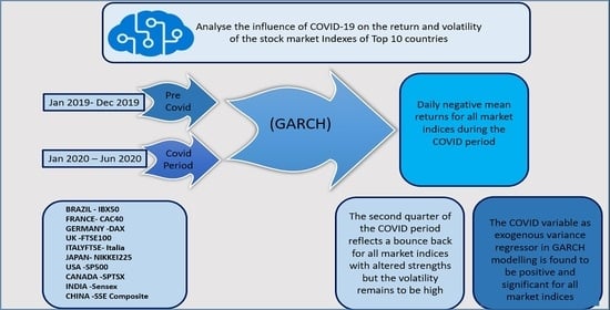
Volatility in International Stock Markets: An Empirical Study during COVID-19

Abstract

Predicting volatility is a must in the finance domain. Estimations of volatility, along with the central tendency, permit us to evaluate the chances of getting a particular result. Financial analysts are frequently challenged with the assignment of diversifying assets in order to form efficient portfolios with a higher risk to reward ratio. The objective of this research is to analyze the influence of COVID-19 on the return and volatility of the stock market indices of the top 10 countries based on GDP using a widely applied econometric model—generalized autoregressive conditional heteroscedasticity (GARCH). For this purpose, the daily returns of market indices from January 2019 to June 2020 were taken into consideration. The results reveal daily negative mean returns for all market indices during the COVID period (January 2020 to June 2020). Though the second quarter of the COVID period reflects a bounce back for all market indices with altered strengths, the volatility remains higher than in normal periods, signaling a bearish tendency in the market. The COVID variable, as an exogenous variance regressor in GARCH modeling, is found to be positive and significant for all market indices. Furthermore, the results confirmed the mean-reverting process for all market indices.

1. Introduction

The contagious COVID-19 disease was first spotted in late 2019 in Wuhan, China and then it was declared as pandemic across the globe and the biggest crisis of this century by the World Health Organization (WHO) in March 2020. The crisis is having a devastating impact that stretches beyond health. The closure/lockdown of countries is leading to a heavier economic price and is now becoming a question of priority between life and livelihood (Bakhshi and Chaudhary 2020). The meagre financial performance of the economy has resulted in a bearish stock market. For any nation, the feel-good factor in the stock market is a key driver that displays the potential return from the capital market in that nation. During an initial crisis period, this feel-good factor quickly turns into a fear factor for shareholders, resulting in a bearish market without much change in the fundamentals of companies (Totir and Dragotă 2011). Hence, analyzing the stock market during the crisis period when the fundamentals of security are diluted by macroeconomic factors is a big challenge (Hoshi and Kashyap 2004) and this challenge is magnificent for any open economy when the financial crisis is due to a pandemic. The nominal GDP of the top 10 countries, i.e., the US, China, Japan, Germany, India, the UK, France, Italy, Brazil, and Canada, adds up to about 66% of the world’s economy and the number of COVID-19 cases in these top 10 countries made up 60% of the total cases as of 15 August 2020. Furthermore, the numbers of COVID-19-positive people are increasing continuously in eight countries in the top 10, i.e., except for China and Japan, and the situation is even worse in America, Brazil and India. Initially, the disease started in China and spilled over to Italy, the UK, France and Germany. As these 10 countries’ economies are illustrative of the world economy and all are affected by COVID-19, this study focuses on impact of COVID-19 on the stock markets of these top 10 countries based on nominal GDP.

The purpose of this paper is to analyze the impact of COVID-19 on the return and volatility of the stock market indices of the top 10 countries based on GDP. These indices are S&P 500—US, Shanghai Composite—China, Nikkie225—Japan, Dax—Germany, BSE Sensex—India, FTSE100—UK, CAC40—France, FTSE Italia All Share—Italy, IBX40—Brazil, and S&PTSX Composite—Canada. Driven by the fear generated by the threat of the virus, this paper represents one of the first efforts to analyze the impact of COVID-19 on the return and volatility of the stock market indices for the top 10 countries based on GDP.

The remaining sections of this paper present a literature review, the methodology of the study, the results, a discussion and the conclusion.

2. Literature Review

The influence of COVID-19 cannot be compared with any previous financial/global crisis or pandemic as the challenges associated with COVID are much greater compared to previous crises. This is mainly due to the fact that we live in a far more integrated world, we have the bottommost historical interest rates, and much greater spillover effects (Fernandes 2020). The current pandemic has the substantial potential to destroy any economy if not managed efficiently (Anjorin 2020; Feinstein et al. 2020) or until there is a vaccine for COVID-19 (Okhuese 2020). The outcome of this pandemic is the slowdown of the economy either due to lockdowns or due to fear resulting in a significantly negative outlook (Onvista 2020). Due to the negative impact of lockdown on many businesses, the total loss can be to the extent of 0.5% of global GDP (Ayittey et al. 2020). Similar estimations have been made by researchers for individual countries like the US (Alfaro et al. 2020), Germany (Michelsen et al. 2020), China (Ruiz and Mario 2020), Saudi Arabia (Albulescu 2020), and many more. The impact of the decrease in the GDP of countries is very much reflected in the financial performance of the stock market. Due to the estimated losses and the fall in stock markets, there is a need for major policy interventions, both fiscal and monetary, and economic aids to protect human health, prevent economic losses and safeguard the financial health of the stock market against COVID-19 (Gourinchas 2020). Apart from these, the International Monetary Fund (IMF) predicted that the COVID-19 pandemic will create the deepest global crisis since the Great Depression (FAZ 2020). Across the world, most of the capital is exchanged through stock markets. Stock market returns are highly influenced by macroeconomic factors (Zahedi and Rounaghi 2015). Hence, the performance of stock markets can impact the domestic economy straightaway. Predictions for stock markets generally tackle the risks of investment in stock markets. Although there are a few challenges in forecasting stock market returns because of false regressions, using different data mining approaches, etc., there is enough literature that proposes that stock market returns possess a foreseeable factor (Campbell and Thompson 2008; Cochrane 2008; Pástor and Stambaugh 2009; Van Binsbergen and Koijen 2010).

Researchers have suggested that the volatility of stock market returns is highly related to uncertainty in the market and hence is the key parameter in most investment decisions/portfolio management decisions. Volatility is the chief risk indicator and an unfailing prediction of stock market volatility is crucial (Green and Figlewski 1999). A greater volatility indicates a significant variation in stock price in the short run. With an increase in volatility, risk increases. A lower volatility indicates that stock prices do not show high variation in the short run and price changes at a stable rate over a certain period of time (Glosten et al. 1993). Higher volatility relates to a greater chance of a bearish market whereas lower volatility relates to greater chances of a bullish market (Ang and Liu 2007). The most commonly used measures of volatility are standard deviation, skewness and kurtosis. The challenge with the primary measure of volatility, standard deviation, is its limitation which is based on the assumption that returns are normally distributed. Skewness works on extremes in the data set rather than concentrating on the average return (Chang et al. 2013). Kurtosis, like skewness, is another measure to be used when the data have extreme values (Mei et al. 2017). The higher moments, i.e., skewness and kurtosis, are also priced in emerging and developed markets. (Fletcher and Kihanda 2005; Teplova and Shutova 2011; and Chaudhary et al. 2020). The Jarque–Bera test is a tool to test goodness-of-fit. If its value is far-off from zero, this indicates that the sample does not possess a normal distribution (Thadewald and Büning 2007). There are some key characteristics of financial time series data that distinguish them from normal time series data and thus differentiate the analysis of financial asset returns from the returns of other classes of assets, i.e., leptokurtic dispersal, volatility clustering, and the effect of leverage. During a financial crisis, the volatility of returns can therefore not be modeled by normal means. Instead, time-varying volatility models are required (Rastogi 2014). The use of the auto regressive conditional heteroscedasticity (ARCH) process to integrate the changing nature of volatility over time was first proposed by Engle (1982), and generalized autoregressive conditional heteroscedasticity (GARCH) models were consequently developed by Bollerslev (1986) to reduce the few shortcomings of ARCH models. The GARCH family of models have been consistently shown to yield the most accurate results and, for this reason, the GARCH system has essentially become the standard method for modeling volatility in financial time series data (Brooks and Rew 2002).

In this work, we analyzed the performance of stock market indices for the top ten major countries across the globe in terms of returns and volatility in the pre-COVID and COVID period by using the GARCH model. The study contributes to the existing literature on international investment markets and it identifies synergies in the markets across the globe. The study also identifies the behavior of different markets in this financial crisis, which is unique, because of its inherent nature. Moreover, it explores the reactions of markets to the crisis and also assesses the trends and behavior of the markets. Thus, this study will help portfolio managers to make well-informed decisions.

3. Data and Methodology

3.1. Data Collection and Market Classification

In this study, the investigation was done by taking daily price data from the Yahoo Finance website on the stock market indices of the top ten countries based on GDP, which includes the United States (S&P 500), China (Shanghai Composite), Japan (Nikkie225), Germany (Dax), India (BSE-Sensex), the United Kingdom (FTSE100), France (CAC40), Italy (FTSE Italia All Share), Brazil (IBX40) and Canada (S&PTSX Composite). These ten countries’ economies constitute 66% of the world GDP and thus can be taken as proxy to represent the overall world economy. The time period taken for the study is from 1 January 2019 to 30 June 2020. The selection of this period was done to incorporate both the pre-COVID period (1 January 2019 to 31 December 2019) and the during COVID period (1 January 2020 to 30 June 2020). The considered period for this study will give a superior comprehension of stock markets’ behavior.

3.2. Estimation Techniques

In this study, the analysis is carried out through various statistical techniques such as Descriptive Statistics, the Unit Root Test, the ARCH effect test and the generalized autoregressive conditional heteroscedasticity (GARCH) (1,1) model (Bhowmik and Wang 2020).

3.2.1. Descriptive Statistics

In this study, Descriptive Statistics include the mean and median as measures of central tendency and standard deviation, and skewness and kurtosis as measures of variability. To confirm normal distribution of returns, the Jarque–Bera test was applied. Time plots of daily returns of market indices have been displayed to give a better insight. A correlation matrix was used to show the correlation coefficient between various market indices. The returns of all the market indices were calculated through the natural log difference approach using the below formula:

$${\mathrm{IR}}_{\mathrm{at}}=\ln (\frac{{\mathrm{P}}_{\mathrm{at}}}{{\mathrm{P}}_{\mathrm{a},\mathrm{t}-1}})$$

(1)

where ${\mathrm{IR}}_{\mathrm{at}}=\mathrm{return}\mathrm{on}\mathrm{index}\mathrm{a}$, ${\mathrm{P}}_{\mathrm{at}}=\mathrm{price}\mathrm{of}\mathrm{index}\mathrm{a}\mathrm{at}\mathrm{the}\mathrm{end}\mathrm{of}\mathrm{the}\mathrm{day}\mathrm{t}$ and ${\mathrm{P}}_{\mathrm{a},\mathrm{t}-1}=\mathrm{price}\mathrm{of}\mathrm{the}\mathrm{index}\mathrm{a}\mathrm{at}\mathrm{the}\mathrm{end}\mathrm{of}\mathrm{the}\mathrm{day}\mathrm{t}-1$.

3.2.2. Unit Root Test

The unit root test is used to check the stationarity of a data series. A time series is said to be stationarity if a shift in time does not cause a change in the shape of the distribution. If the series is found to be stationary, it indicates that mean, variance and auto correlation structure do not change over a period of time. To check this, the Augmented Dickey–Fuller Test was applied in which a null hypothesis was hypothesized as the existence of a unit root (Dickey and Fuller 1981).

${\mathrm{H}}_0$ = There exists a unit root

$$\Delta {\mathrm{y}}_{\mathrm{t}}={\propto }_0+{\mathsf{\theta }\mathrm{y}}_{\mathrm{t}-1}+{\displaystyle \sum }_{\mathrm{i}=1}^{\mathrm{n}}\propto \Delta {\mathrm{y}}_{\mathrm{t}}+{\mathrm{e}}_{\mathrm{t}}$$

(2)

where ‘y’ indicates the time series, ‘t’ is the time period, ‘n’ is the optimum number of lags, ‘α₀’ is called the constant value and ‘e’ is known as the error term.

3.2.3. ARCH Effect Test

The auto regressive conditional heteroscedasticity–Lagrange Multiplier Test (ARCH–LM) was used to check for heteroscedasticity, for residuals and to check the presence of the ARCH/GARCH effect Engle (1982).

To test for ARCH of order p, the following auxiliary regression model was used

$${\mathrm{u}}_{\mathrm{t}}^2={\mathsf{\gamma }}_0+{\mathsf{\gamma }}_1{\mathrm{u}}_{\mathrm{t}-1}^2+{\mathsf{\gamma }}_2{\mathrm{u}}_{\mathrm{t}-2}^2+\dots +{\mathsf{\gamma }}_{\mathrm{p}}{\mathrm{u}}_{\mathrm{t}-\mathrm{p}}^2+{\mathrm{v}}_{\mathrm{t}}$$

(3)

where ‘$\mathrm{u}$’ is called the square residual, which can be measured by the primary regression model; however, in a secondary regression model, ‘p’ lags are incorporated.

The null hypothesis in this test is that there is no ARCH effect:

$${\mathrm{H}}_0={\mathsf{\gamma }}_0={\mathsf{\gamma }}_1={\mathsf{\gamma }}_2={\mathsf{\gamma }}_{\mathrm{p}}=0$$

(4)

3.2.4. GARCH Model

The generalized ARCH (GARCH) is an extension of the ARCH model. A GARCH model might have lesser parameters compared to an ARCH model. The GARCH family of models have been regularly shown to give more precise outcomes and, because of this, the use of the GARCH model has become the standard method for modeling volatility in financial time series data. The GARCH (p, q) model can be enumerated as follows (Brooks and Rew 2002):

Conditional Mean Equation

$${\mathrm{y}}_{\mathrm{t}}=\mathsf{\mu }+\mathrm{t}$$

(5)

Conditional Variance Equation

$${\mathrm{h}}_{\mathrm{t}}^2=\mathsf{\omega }+{\displaystyle \sum }_{\mathrm{i}=1}^{\mathrm{q}}{\mathsf{\alpha }}_{\mathrm{i}}{\mathsf{\epsilon }}_{\mathrm{t}-\mathrm{i}}^2+{\displaystyle \sum }_{\mathrm{i}=1}^{\mathrm{p}}{\mathsf{\beta }}_{\mathrm{i}}{\mathrm{h}}_{\mathrm{t}-\mathrm{i}}^2$$

(6)

where y_t is the conditional mean, h_t is the conditional variance, ω and μ are the constant terms, t is the error term of the mean equation, and q and p are the lag of the residual (error) term and conditional variance terms in the conditional variance equation.

The simplest but often most relevant GARCH process is the GARCH (1,1) model, also known as the generic or ‘plain vanilla’ GARCH model. Karmakar (2005) has recommended the use of GARCH (1,1) to record conditional volatility in stock returns. The GARCH (1,1) model is written as follows, where p = 1 and q = 1, and where Equation (6) gets transformed into Equation (7):

$${\mathrm{h}}_{\mathrm{t}}^2=\mathsf{\omega }+{\mathsf{\alpha }}_1{\mathsf{\epsilon }}_{\mathrm{t}-1}^2+{\mathsf{\beta }}_1{\mathrm{h}}_{\mathrm{t}-1}^2$$

(7)

In Equation (7), α₁ and β₁ are the coefficients of the ARCH and GARCH terms, respectively, where ‘α’ (ARCH effect) estimates the response to shock and ‘β’ (GARCH effect) quantifies the time it takes for any change to die away. Greater α values depict higher sensitivity to new information, while greater β values depict a greater amount of time for the change to die out. (α + β) provide a measure of the persistence of the relevant time series and thus higher values for (α + β) should tend towards one and imply greater persistence in volatility (Rastogi 2014).

3.2.5. GARCH Model with Exogenous Volatility Regressors

It is important to gauge the impact of COVID on the mean return and volatility process. The model has been extended by including a dummy variable for the COVID period to identify the significance of the period.

Conditional Mean Equation

$${\mathrm{y}}_{\mathrm{t}}=\mathsf{\mu }+{\mathsf{\lambda }}_1{\mathrm{COVID}}_{\mathrm{t}}+\mathrm{t}$$

(8)

Conditional Variance Equation

$${\mathrm{h}}_{\mathrm{t}}^2=\mathsf{\omega }+{\mathsf{\alpha }}_1{\mathsf{\epsilon }}_{\mathrm{t}-1}^2+{\mathsf{\beta }}_1{\mathrm{h}}_{\mathrm{t}-1}^2+{\mathsf{\delta }}_1{\mathrm{COVID}}_{\mathrm{t}}$$

(9)

The dummy variable COVID assumes a value of 0 for the pre-coronavirus period (1 January 2019–31 December 2019) and 1 for the current coronavirus period (i.e., 1 January 2020 to 30 June 2020). Therefore, in the conditional mean equation, a negative and statistically significant coefficient for COVID would indicate a correlation between coronavirus and a reduction in the mean returns of the markets, while a positive and statistically significant coefficient for COVID would indicate a correlation between coronavirus and an increase in the mean returns of the market. In the conditional variance equation, a negative and statistically significant coefficient for COVID would indicate a correlation between coronavirus and a reduction in the volatility of the markets, while a positive and statistically significant coefficient for COVID would indicate a correlation between coronavirus and an increase in the volatility of the market.

4. Empirical Results

Table 1. (A–D): Descriptive Statistics.

Particulars	SP500	SSE Composite	NIKKEI225	DAX	SENSEX	FTSE100	CAC40	FTSE Italia	IBX50	SPTSX Composite
	US	CHINA	JAPAN	GERMANY	INDIA	UK	FRANCE	ITALY	BRAZIL	CANADA
(A). 12-month period before crisis (January 2019–December 2019)
Mean	0.0010	0.0008	0.0007	0.0009	0.0005	0.0004	0.001	0.0009	0.0009	0.0007
Median	0.0009	0.0001	0.0005	0.0013	0.0001	0.0007	0.0016	0.001	0.0015	0.0007
Maximum	0.0338	0.0545	0.0258	0.0331	0.0519	0.0223	0.0269	0.0308	0.0286	0.0149
Minimum	−0.0302	−0.0575	−0.0305	−0.0316	−0.0208	−0.0328	−0.0364	−0.028	−0.0386	−0.0188
Std. Dev.	0.0078	0.0111	0.0085	0.0088	0.0084	0.0074	0.0084	0.0089	0.0112	0.0046
Skewness	−0.6364	−0.177	−0.1006	−0.353	1.2011	−0.4429	−0.7383	−0.435	−0.537	−0.4928
Kurtosis	6.272	8.4057	4.4235	4.9843	9.0003	5.1677	5.5685	4.2787	3.9284	4.3354
Jarque–Bera	130.45	310.59	21.87	46.95	442.12	58.03	92.89	25.31	21.33	29.15
Probability	0	0	0	0	0	0	0	0	0	0
Observations	254	254	254	254	254	254	254	254	254	254
(B). 6-month period during crisis (January 2020–June 2020)
Mean	−0.0003	−0.0002	−0.0005	−0.0006	−0.0013	−0.0016	−0.0015	−0.0015	−0.0016	−0.0008
Median	0.0018	0.0002	0.0000	0.0006	0.0000	0.0007	0.0008	0.0025	0.0000	0.0021
Maximum	0.0897	0.0310	0.0773	0.1041	0.0859	0.0867	0.0806	0.0800	0.1371	0.1129
Minimum	−0.1277	−0.0804	−0.0627	−0.1305	−0.1410	−0.1151	−0.1310	−0.1791	−0.1625	−0.1318
Std. Dev.	0.0290	0.0132	0.0203	0.0265	0.0270	0.0235	0.0261	0.0280	0.0387	0.0287
Skewness	−0.6235	−2.0292	0.2865	−0.7791	−1.2375	−0.9446	−1.1542	−2.4367	−1.0127	−1.0016
Kurtosis	7.2982	13.3265	5.6055	8.7433	9.6166	8.1969	8.0873	16.7166	8.3742	10.3186
Jarque–Bera	105.15	646.32	37.36	185.92	262.00	160.53	163.85	1112.45	173.17	302.26
Probability	0	0	0	0	0	0	0	0	0	0
Observations	126	126	126	126	126	126	126	126	126	126
Particulars	SP500	SSE Composite	NIKKEI225	DAX	SENSEX	FTSE100	CAC40	FTSE Italia	IBX50	SPTSX Composite
	US	CHINA	JAPAN	GERMANY	INDIA	UK	FRANCE	ITALY	BRAZIL	CANADA
(C). First quarter during crisis (January 2020–March 2020)
Mean	−0.0035	−0.0016	−0.0035	−0.0045	−0.0053	−0.0045	−0.0048	−0.0050	−0.0074	−0.0038
Median	0.0000	0.0000	−0.0007	−0.0003	−0.0031	0.0000	−0.0002	0.0011	−0.0028	0.0014
Maximum	0.0897	0.0310	0.0773	0.1041	0.0675	0.0867	0.0806	0.0800	0.1371	0.1129
Minimum	−0.1277	−0.0804	−0.0627	−0.1305	−0.1410	−0.1151	−0.1310	−0.1791	−0.1625	−0.1318
Std. Dev.	0.0356	0.0171	0.0228	0.0294	0.0310	0.0272	0.0299	0.0342	0.0488	0.0369
Skewness	−0.4411	−1.6899	0.6256	−0.9262	−1.5319	−0.9302	−1.2645	−2.3461	−0.7253	−0.7052
Kurtosis	5.7551	8.7859	6.1385	9.7816	8.6145	8.1518	8.0128	13.6953	5.9901	7.1198
Jarque–Bera	22.32	119.73	30.44	131.79	109.09	80.01	84.06	363.75	29.45	50.57
Probability	0	0	0	0	0	0	0	0	0	0
Observations	64	64	64	64	64	64	64	64	64	64
(D). Second quarter during crisis (April 2020–June 2020)
Mean	0.0029	0.0013	0.0026	0.0035	0.0027	0.0014	0.0019	0.0021	0.0045	0.0024
Median	0.0045	0.0009	0.0000	0.0034	0.0031	0.0029	0.0035	0.0035	0.0044	0.0032
Maximum	0.0680	0.0219	0.0477	0.0561	0.0859	0.0420	0.0503	0.0363	0.0637	0.0493
Minimum	−0.0608	−0.0191	−0.0461	−0.0457	−0.0612	−0.0407	−0.0482	−0.0478	−0.0575	−0.0423
Std. Dev.	0.0199	0.0072	0.0170	0.0225	0.0215	0.0188	0.0212	0.0193	0.0230	0.0162
Skewness	−0.2735	0.3682	−0.1089	−0.0788	0.3333	−0.3842	−0.2874	−0.5957	0.0332	−0.3855
Kurtosis	5.0503	4.2192	3.7746	2.9594	6.2074	2.7024	3.0523	2.9953	2.9517	4.2579
Jarque–Bera	11.63	5.24	1.67	0.07	27.72	1.75	0.86	3.67	0.02	5.62
Probability	0.003	0.073	0.433	0.966	0.000	0.416	0.650	0.160	0.991	0.060
Observations	62	62	62	62	62	62	62	62	62	62

presents a summary of the Descriptive Statistics of daily returns for all indices of the top 10 countries by GDP. The entire period of study from January 2019 to June 2020 was divided into two, the pre-COVID-19 period (1 January 2019–31 December 2019) (Table 1 Part (A)) and the COVID-19 period (1 January 2020–30 June 2020) (Table 1 Part (B)). Furthermore, the COVID-19 period was subdivided into two quarters, as presented in part (C) and part (D) of Table 1.

The daily returns of all indices during the COVID-19 period (January 2020–June 2020) show negative mean returns while the pre-COVID-19 period (January 2019–December 2019) has positive daily mean returns. Furthermore, the first quarter of the COVID-19 crisis depicts negative mean returns for all indices and the second quarter of the crisis shows positive mean returns for all indices, showing the negative market reaction to be strong in the early days of the crisis. It is observed that the minimum value of all indices during the crisis period (January 2020–June 2020) was in the month of March 2020. Only the SSE Composite index of China has a minimum value (−8.04%) on 3 February 2020. The biggest one-day plunge is seen in the FTSE Italia All Share Index of Italy (−17.91%) accompanied by the IBX50 Index of Brazil (−16.25%) on 12th March 2020 and in Sensex of India (−14.10%) on 23rd March 2020. The primary measure of risk, i.e., the standard deviation, is quite large for all indices during the COVID-19 period compared to the pre-COVID-19 period. Though the mean daily returns of second quarter of COVID-19 crisis period are positive and show a significant bounce back compared to the first quarter of COVID-19 crisis period, at the same time, all indices show large values of standard deviation compared to the pre-COVID-19 period. In general, all indices are showing higher negative skewness during the COVID-19 crisis period compared to the pre-COVID-19 crisis period. Comparing pre-COVID-19 and during the COVID-19 crisis period, all indices show a higher kurtosis value, indicating a leptokurtic distribution of returns. It is also observed that the second quarter of the COVID-19 crisis period show lower negative skewness and lower kurtosis values of return distribution compared to the first quarter of the COVID-19 crisis period. The Jarque–Bera test confirms the returns be abnormal in both the pre-COVID-19 period and during the COVID-19 period. Furthermore, some indices in the second quarter of the COVID-19 crisis show normality return, but, at the same time, all indices in the same period show an increased standard deviation compared to normal periods.

Table 2. Highlights of periodic returns.

Indices	Periodic Returns (%)
	January–December 2019	July–December 2019	January–June 2020	January–March 2020	April–June 2020
	(12 Months before Crisis)	(6 Months before Crisis)	(6 Months—During Crisis)	(First 3 Months (1st Quarter) during Crisis)	(Next 3 Months (2nd Quarter) during Crisis)
SP500 (US)	28.71	9.82	1.25	−20.00	26.56
SSE Composite (CHINA)	23.72	2.39	8.52	−9.83	20.35
NIKKEI225 (JAPAN)	18.20	11.19	−8.23	−20.04	14.76
DAX (GERMANY)	25.22	6.86	−7.06	−25.01	23.93
SENSEX (INDIA)	14.94	4.72	−8.84	−28.57	27.62
FTSE100 (UK)	12.00	1.57	−21.81	−24.80	3.98
CAC40 (FRANCE)	27.48	7.93	−19.98	−26.46	8.82
FTSE Italia All Share (ITALY)	27.02	10.66	−18.49	−27.54	12.49
IBX50 (BRAZIL)	24.74	13.17	−11.06	−37.60	42.53
SPTSX Composite (CANADA)	18.93	4.16	−5.24	−21.59	20.86

contains the highlights of periodic returns for semi-annual periods, one during the crisis (January–June 2020) and the other before the crisis period (July–December 2019), controlling for equal window lengths for the period. Furthermore, the periodic returns of the first and second quarter, of the crisis period, and the annual return of 2019 are also displayed in the table separately.

The table reveals that the indices of the UK (−21.81%), France (−19.98%) and Italy (−18.49%) did the poorest in relation to periodic returns from January to June 2020. The markets of China and the US are the only markets showing positive returns for the period of January to June 2020. Comparing the periodic returns of the second quarter with the first quarter of 2020, it is significantly evident that all the economic indices have bounced back with altered strengths. Overall, the British and French indices had the weakest rebound relatively, while Brazil, India and the US market indices exhibited the strongest strength in their rebound.

Figure 1 shows the daily returns of all the indices over the period from January 2019 to June 2020. The graphs in Figure 1 provide an insight into the high volatility during the current coronavirus period with all ten countries’ market indices taken into consideration. Furthermore, all the graphs seem to exhibit volatility clustering, so volatility in the current period will affect future periods of volatility, and all return series seem to be mean reverting, which signifies stationarity.

Table 3. Correlation Matrix of Market Indices.

(A): Correlation Matrix of Market Indices-Period (January 2019–31 December 2019)
	BRAZIL IBX50	FRANCE CAC40	GERMANY DAX	UK FTSE100	ITALY FTSE Italia	JAPAN NIKKEI225	USA SP500	CANADA SPTSX	INDIA Sensex	CHINA SSE Composite
BRAZIL IBX50	1.000	0.330	0.305	0.294	0.263	0.010	0.470	0.363	0.040	0.010
FRANCE CAC40	0.330	1.000	0.909	0.779	0.840	0.187	0.730	0.655	0.132	0.248
GERMANY DAX	0.305	0.909	1.000	0.704	0.822	0.189	0.691	0.607	0.118	0.280
UK FTSE100	0.294	0.779	0.704	1.000	0.606	0.202	0.628	0.556	0.143	0.229
ITALYFTSE Italia	0.263	0.840	0.822	0.606	1.000	0.115	0.671	0.610	0.056	0.279
JAPAN NIKKEI225	0.010	0.187	0.189	0.202	0.115	1.000	0.133	0.145	0.165	0.365
USA SP500	0.470	0.730	0.691	0.628	0.671	0.133	1.000	0.735	0.108	0.181
CANADA SPTSX	0.363	0.655	0.607	0.556	0.610	0.145	0.735	1.000	0.104	0.156
INDIA Sensex	0.040	0.132	0.118	0.143	0.056	0.165	0.108	0.104	1.000	0.167
CHINA SSE Composite	0.010	0.248	0.280	0.229	0.279	0.365	0.181	0.156	0.167	1.000
(B): Correlation Matrix of Market Indices-Period (January 2020–30 June 2020)
	BRAZIL IBX50	FRANCE CAC40	GERMANY DAX	UK FTSE100	ITALY FTSE Italia	JAPAN NIKKEI225	USA SP500	CANADA SPTSX	INDIA Sensex	CHINA SSE Composite
BRAZIL IBX50	1.00	0.73	0.69	0.72	0.69	0.33	0.82	0.85	0.53	0.34
FRANCE CAC40	0.73	1.00	0.97	0.95	0.91	0.51	0.74	0.81	0.63	0.39
GERMANY DAX	0.69	0.97	1.00	0.94	0.91	0.53	0.73	0.80	0.57	0.37
UK FTSE100	0.72	0.95	0.94	1.00	0.89	0.48	0.75	0.84	0.62	0.39
ITALY FTSE Italia	0.69	0.91	0.91	0.89	1.00	0.42	0.72	0.79	0.56	0.29
JAPAN NIKKEI225	0.33	0.51	0.53	0.48	0.42	1.00	0.33	0.40	0.35	0.49
USA SP500	0.82	0.74	0.73	0.75	0.72	0.33	1.00	0.89	0.45	0.30
CANADA SPTSX	0.85	0.81	0.80	0.84	0.79	0.40	0.89	1.00	0.56	0.38
INDIA Sensex	0.53	0.63	0.57	0.62	0.56	0.35	0.45	0.56	1.00	0.53
CHINA SSE Composite	0.34	0.39	0.37	0.39	0.29	0.49	0.30	0.38	0.53	1.00

A,B present the correlation between all indices for the period January 2019–December 2019 and from January 2020 to June 2020, respectively.

As observed from the correlations in Table 3, a positive correlation across all markets is seen. As the world is coming closer and more integrated, the financial capital flows across different economies and thus markets across the globe tend to depend heavenly on each other. This economic integration has led to portfolio managers diversifying across the globe, which has also led to the spreading of risk from one economy to others. Furthermore, it can be seen, when comparing Table 3A to Table 3B, that positive correlations across the markets have increased in the crisis period, indicating the stickiness and dependencies across the markets. This manifestation, that the stock markets across the globe become much more cohesive due to any turbulence in the economy, is best called the ‘contagion effect’ (Roll 1989). An increase in the degree of cohesiveness during and after a crisis compared to the cohesiveness before a crisis was reported by Huyghebaert and Wang (2010) and Akter and Nobi (2018).

In this paper, the GARCH (1,1) model for the analysis of financial time series data of all ten country market indices was investigated. The necessary conditions of stationarity and the ARCH effect test were employed. The Augmented Dickey–Fuller (ADF) test was used in this paper to test for a unit root and the ARCH–LM test was used to check for heteroscedasticity and for residuals.

Table 4. Results of Augmented Dickey–Fuller test and the ARCH–LM test.

Particulars	SP500	SSE Composite	NIKKEI225	DAX	SENSEX	FTSE100	CAC40	FTSE Italia	IBX50	SPTSX Composite
	US	CHINA	JAPAN	GERMANY	INDIA	UK	FRANCE	Italy	BRAZIL	CANADA
ADF in Level T-Statistics	−5.12 *	−19.98 *	−17.89 *	−19.15 *	−7.81 *	−6.14 *	−6.07 *	−8.74 *	−24.94 *	−5.67 *
ARCH Effects Obs *R-squared	97.02 *	6.14 **	100.03 *	3.08 ***	11.15 *	7.23 **	2.95 ***	6.61 **	137.23 *	68.10 *

* Significant at 1% level; ** significant at 5% level; *** significant at 10% level.

presents the results of the Augmented Dickey–Fuller test and the ARCH–LM test. As Table 4 shows, all the indices in level form have a higher test statistic than critical value; thus, the null hypothesis of the presence of a unit root is rejected and, furthermore, it is concluded that the indices are stationary in their level form at the one percent level. The probability values of LM statistics are also found to be significant, thus rejecting the null hypothesis of no ARCH effect. This confirms the presence of the ARCH effect in the residuals of the time series model of the returns. Thus, the pre-conditions for using the plain vanilla GARCH (1,1) model were satisfied.

The results of plain vanilla GARCH (1,1) for all economic indices are presented in

Table 5. Results of generalized autoregressive conditional heteroscedasticity (GARCH) (1,1).

Particulars	SP500	SSE Composite	Nikkei 225	DAX	SENSEX	FTSE100	CAC40	FTSE Italia All Share	IBX50	SPTSX Composite
	US	CHINA	JAPAN	GERMANY	INDIA	UK	FRANCE	Italy	BRAZIL	CANADA
μ	0.001421 (3.6670) *	0.000597 (1.8898) ***	0.000612 (1.9138) ***	0.001209 (2.2218) **	0.000735 (1.6411) ***	0.000434 (1.9809) **	0.001277 (2.5728) *	0.001173 (2.0104) **	0.001295 (1.7518) ***	0.000816 (3.1722) *
ω	3.56 × 10−6 (2.7448) *	5.65 × 10−6 (3.5623) *	6.50 × 10−6 (2.4750) **	5.95 × 10−6 (3.4837) *	4.34 × 10−6 (2.3893) **	4.38 × 10−6 (2.6213) *	6.59 × 10−6 (4.0498) *	7.37 × 10−6 (3.3056) *	1.21 × 10−5 (3.6355) *	1.69 × 10−6 (3.1080) *
α (ARCH Effect)	0.33913 (6.8665) *	0.054928 (3.1125) *	0.104624 (4.3028) *	0.219208 (6.0794) *	0.181486 (5.6950) *	0.248892 (4.9897) *	0.291955 (5.7757) *	0.238317 (6.3225) *	0.143088 (6.4513) *	0.375565 (8.0774) *
β (GARCH Effect)	0.650143 (18.8833) *	0.90837 (39.6550) *	0.8499 (22.6152) *	0.773193 (22.2517) *	0.810802 (23.2662) *	0.749362 (15.9746) *	0.701376 (15.3047) *	0.755434 (18.205) *	0.822506 (32.1667) *	0.622711 (16.9583) *
α + β	0.989273	0.963298	0.954594	0.992401	0.992288	0.998254	0.993331	0.993751	0.965594	0.998276
Log likelihood	1210.105	1158.017	1167.572	1141.244	1169.975	1204.38	1168.252	1134.892	1048.493	1362.702
Schwarz criterion	−6.306446	−6.0323	−6.08259	−5.944018	−6.09524	−6.276312	−6.08617	−5.91059	−5.455854	−7.10959

Note Figures in ( ) indicate the value of Z-statistics. * Significant at 1% level; ** significant at 5% level; *** significant at 10% level.

. The conditional mean equation coefficient for all indices are positive and statistically significant. In the variance equation, the coefficient of the constant variance term and the ARCH and GARCH parameters are positive and statistically significant for all the indices. The coefficients in the conditional variance equation, i.e., α (ARCH effect) and β (GARCH effect), both relate to news. Specifically, α represents recent news, and its value here is statistically significant, which implies that recent news has impacted stock market volatility. β represents old news, and the fact that its value is also statistically significant indicates that old news has also impacted market volatility. Furthermore, large GARCH coefficients signify that shocks to conditional variance are taking a long time to die away and that volatility is thus ‘persistent’. Table 5 reveals that the sum of the ARCH and the GARCH coefficients (α + β) is close to one. If α + β is close to unity, then a ‘shock’ at time t will remain for a long time to come. In other words, a high value for α + β implies a ‘long memory’, and any shock may lead to a permanent change in the future values of h_t, indicating that conditional variance is persistent. At the same time, the results show a mean-reverting process, as the sum of the coefficients of alpha and beta is less than one. Furthermore, the absolute value, α + β, controls the speed of mean reversion. It is evident from the results that the SPTSX Composite (Canada) and FTSE 100 (UK) have the slowest mean reversion, implying a volatility half-life of about 402 and 397 days, respectively, whereas Nikkei 225 (Japan) and SSE Composite (China) have the fastest mean reversion, implying a volatility half-life of about 15 and 19 days, respectively. Based on the results of the GARCH model, the null hypothesis of no change in volatility can be rejected. Instead, the change in volatility has been shown to be significant.

Table 6. Results of GARCH (1,1) with COVID variable.

Particulars	SP500	SSE Composite	NIKKEI225	DAX	SENSEX	FTSE100	CAC40	FTSE Italia All Share	IBX50	SPTSX Composite
	US	CHINA	JAPAN	GERMANY	INDIA	UK	FRANCE	Italy	BRAZIL	CANADA
Conditional Mean Equation
μ	0.001358 (3.5688) *	0.000661 (1.6108) ***	0.000742 (1.6707) ***	0.001077 (1.8806) **	0.000842 (1.8185) ***	0.000523 (1.6348) ***	0.001226 (2.1979) **	0.001020 (1.6587) **	0.001166 (1.6676) ***	0.000670 (2.6169) *
λ (COVID)	−1.08 × 10−5 (−0.0068)	−0.000490 (−0.2773)	−0.000362 (−0.2085)	8.89 × 10−5 (0.0462)	−0.000893 (−0.5862)	−0.000913 (−0.5622)	−0.000754 (−0.4362)	0.000479 (0.2328)	0.000230 (0.0942)	0.000965 (1.0261)
Conditional Variance Equation
ω	3.40 × 10−6 (2.4772) **	3.82 × 10−6 (2.5679) **	2.70 × 10−5 (3.0993) *	5.73 × 10−6 (3.3089) *	4.43 × 10−6 (2.3452) **	4.61 × 10−6 (2.6982) *	6.14 × 10−6 (3.5652) *	7.22 × 10−6 (2.4350) **	1.69 × 10−5 (2.5337) **	1.46 × 10−6 (2.7331) *
α (ARCH Effect)	0.268420 (4.9082) *	0.061352 (3.7319) *	0.1444 (3.0515) *	0.151716 (5.2980) *	0.164587 (5.3907) *	0.198332 (4.2870) *	0.213614 (5.2521) *	0.140363 (4.0843) *	0.149000 (4.2739) *	0.372955 (7.0550) *
β (GARCH Effect)	0.705961 (14.7775) *	0.905009 (48.2772) *	0.506521 (3.6505) *	0.791617 (21.6699) *	0.803235 (20.7108) *	0.757320 (13.0385) *	0.737072 (14.6827) *	0.789942 (13.6004) *	0.743219 (10.4432) *	0.625084 (15.4048) *
δ (COVID)	1.77 × 10−5 (3.0597) *	5.70 × 10−6 (4.5694) *	8.33 × 10−5 (2.3764) **	2.57 × 10−5 (2.8049) *	1.15 × 10−5 (2.1761) **	1.33 × 10−5 (2.0323) **	1.95 × 10−5 (2.8251) *	2.98 × 10−5 (2.61102) *	5.55 × 10−5 (2.7173) *	1.98 × 10−6 (1.2939)
α + β	0.974381	0.966361	0.650921	0.943333	0.967822	0.955652	0.950686	0.930305	0.892219	0.998039
Log likelihood	1215.082	1161.873	1177.034	1146.832	1173.180	1207.690	1172.123	1139.949	1058.405	1364.704
Schwarz criterion	−6.301378	−6.021327	−6.101124	−5.942166	−6.080841	−6.262469	−6.075275	−5.905938	−5.476761	−7.088860

Note Figures in ( ) indicate the value of Z-statistics. * Significant at 1% level; ** significant at 5% level; *** significant at 10% level.

presents the results of the GARCH (1,1) model, which adds the coronavirus variable to the conditional mean and conditional variance equation. The results reveal a significant positive impact of the virus on the conditional variance for all the indices (except the SPTSX Composite Index of Canada where Z-statistics are not significant but the value is still greater than one), indicating that COVID-19 increased market volatility in all these indices. These results confirm those of Ibrahim Yousef (2020) who also found that COVID-19 is positively and significantly related to equity return volatility in the context of the US market. Furthermore, it is also seen that the coronavirus variable has no impact on the mean returns.

5. Discussion and Conclusions

The current empirical study attempts to analyze the impact of COVID-19 on the performance of the top 10 stock indices of the global economy, as measured by GDP. Daily data from January 2019 to June 2020 were considered in this study. The Descriptive Statistics reveal daily negative mean returns in the COVID period (January to June 2020). It is evident from the data that the second quarter of the crisis shows daily positive mean returns for all indices, showing a bounce back, but these returns have a higher standard deviation compared to normal periods. The daily return data exhibit negative skewness and higher kurtosis during the crisis period. Furthermore, the correlation matrix shows an increase in the degree of cohesiveness between all market indices during the COVID period.

The question that arises here is: how can all of the world indices rally despite the catastrophic dip in March? Despite a rise in COVID-19 cases, the decline in the GDP growth rate and the decline in the gross fixed capital formation as a percentage of GDP, worldwide markets have seen a sharp recovery. Given the inherent uncertainty in the current environment, however, it is difficult to predict the long-term economic impact of COVID-19, especially since there is no comparable historical benchmark on which to base such predictions. The fact that the market is a self-correcting system and that participants in the ecosystem can prophesize its fluctuations with remarkable precision may provide probable reasons for the rally that is shown by all the world indices in the second quarter (April–June 2020), despite the somber economic projections everywhere. Another explanation is that all of this is simply a byproduct of irrational exuberance (Schiller 2015). According to Robert Schiller, this is the psychosomatic base of a speculative bubble. A speculative bubble is a condition in which news of price upsurges translate into irrational stockholder eagerness. It spreads just like a virus. In the process, each individual amplifies the story, justifies the price increase, and ropes in more participants. These people might be drawn to the euphoria partly by envy of others’ successes and partly through gamblers’ excitement. While these explanations might be convincing to some, it is also prudent to note that very few economists expect to see a sharp bounce back. This means that the whole hypothesis might be suspect. This study supports the suspicion about the above hypothesis, as the second quarter positive daily mean returns are accompanied by higher volatilities and higher volatilities relate to a greater chance of a bearish market, whereas lower volatility relates to greater chances of a bullish market. The same finding was confirmed by Ang and Liu (2007). In summary, it is simply a bubble waiting to explode.

The results of the GARCH (1,1) model expose that the COVID-19 coefficient in the conditional variance equation has a substantial positive influence on conditional variance for all the indices, which indicates that the virus has increased the volatility in these indices. It can be further stated from the research output that all ten markets witness a mean-reverting procedure as the sum of the ARCH and GARCH coefficient is lower than one. Ahmed et al. (2018), Mishra (2017) and Tripathy (2017) also found similar results. As the received outcome shows a mean reversion procedure in all ten stock markets, the stock returns of all the ten markets return back to the previous mean values after a certain period of time. The mean reversion occurrence offers a chance for investors to predict the future price of the security, bearing in mind its past values. Further scope for this research entails considering the more vigorous techniques and asymmetric volatility models like threshold ARCH (TARCH), which include signs implying the invention of volatilities, which can impact the variation in stock returns, and to exploring stock market integration.