Portfolio Theory in Solving the Problem Structural Choice

Abstract

The purpose of the article is to reveal the problem (and to determine the possibility of solving the structural choice problem) as one of the areas in modern portfolio theory development. The article also argues that portfolio analysis is a method of structural analysis for various economic units. The research methodology is defined by the portfolio theory, optimization models implemented by the numerical gradient projection method, the empirical static method of analysis and simulation cases when the models are implemented. The research supported by the above- mentioned methodology aimed to reach the goal results in substantiating the structural choice. This choice differs from the classical portfolio choice as it is necessary to find how the investments are allocated for the portfolio units, and the same should be done for the characteristics points, where it is a challenge to apply the efficient set theorem, because different structures for the allocation of the resources, investments give the same or nearly the same combination of the expected return and total portfolio risk. Economic sectors characterized by the profitability and business risk are seen to be the portfolio units in terms of the macroeconomic approach from the portfolio theory developed by Tobin. Total income maximization model and total portfolio risk minimization demonstrate both the structural choice problem, including at the characteristic points, and choice dependence on the expansion of the resource allocated to the portfolio, and on the number of portfolio units. The analysis and model simulations enhance the efficient set theorem with the criteria for structural choice—income and risk correlation on the effective distribution curve, among other factors. A portfolio with two real sectors of the Russian economy illustrates that profitability and risk ratio determines the resource allocation between them under the income maximization model, so one sector grabs a more substantial resource. Thus, being a tool to support the structural choice, portfolio analysis gives structural diagnostics for the resource distribution, investments allocation by portfolio units.

1. Introduction. Portfolio Theory: Past and Present

Originated from the classical works by H. Markowitz, J. Tobin, and W. Sharpe (Markowitz 1952, 1959, 1991; Markowitz and Dijk 2008; Tobin 1955; Sharpe 1970; Sharpe et al. 1998), modern portfolio theory has gone a long way in its development, and has become an independent scientific domain, which gives both theoretical and very useful practical results.

Portfolio theory development resulted in delivering special academic courses, in publishing textbooks (Sharpe et al. 1998; Satchell 2016), which indicate the importance of this scientific area. If we analyze the history of portfolio theory development in the second half of the twentieth century, it is possible to divide this theory into two sections (in addition to the normative and positive theory (Markowitz 1991) with its own field of application and emerging tasks1.

The first task is to study the portfolio choice problems originated from H. Markowitz and W. Sharpe (Sharpe 1970; Markowitz and Dijk 2008; Grant and Satchell 2020) regarding both financial assets and their combinations with others assets (Byers et al. 2015). This task also covers various ways to improve quantitative assessments of risk and return, to conduct statistical research aimed at confirming the correlation between relevant portfolio parameters (Li and Mei 2014; Cuchiero 2019; Fu and Blazenko 2017; Fahmy 2020), and to improve optimization algorithms (Esfahani et al. 2016). What is more, the diversification of securities and other financial assets portfolio are examined (Lhabitant 2017) to build portfolios with regard to portfolio profitability and risk correlation, investors’ disposition to risks, the application of optimization methods as tools for solving portfolio tasks with financial assets (Romeo 2020).

The second task is to analyze the portfolio choice at the macroeconomic level, originated from J. Tobin (Tobin 1955; Kumhof 2018; van Bilsen and Laeven 2020; Puntsag 2020), in the view of various aspects of macroeconomic development or portfolio choice in certain types of activities (Alvarez et al. 2017; Zhang et al. 2018; Moser et al. 2017; Carmona et al. 2020). This level of analysis allows us to study the investors’ choice between physical and monetary capital, and a much wider choice among more portfolio units and different behavior patterns of the choice agents. Here, portfolio theory clearly expands its scope as a structural analysis method and even structural change management method (Brainard and Tobin 1992).

The latter version of the portfolio theory, which develops the tradition of portfolio analysis by J. Tobin, can be significantly expanded for the analysis of monetary issues—the demand for money (Serletis 2001), investment and debt ratio (Nkeki 2018) during a financial crisis, or sectoral economic structure—the investments allocation for the actual units (sectors), which is the ultimate purpose of the article.

Both tasks involve the optimization modeling aimed to maximize the function of the total expected return and risk. However, the optimization problem can be represented as a structural choice problem, in other words, obtaining a vector of investments allocation, resources distribution across portfolio units with the highest income and the lowest risk. It is necessary to note that financial portfolios, as well as portfolios with the real units make these goals ambiguous. This rises the structural choice problem at the level of the target optimization functions, not to mention the fact that it will probably be necessary to adjust the obtained solutions to the optimization models. At the same time, if we are talking about conditional optimization, it is necessary to optimize the functions under the identical conditions. Otherwise, it will be necessary to interpret the discrepancy arising from the optimization of conflicting goals (income and risk) and even with significantly different restrictions.

The classical portfolio theory is based on the efficient set theorem, which does not clarify all the nuances in structural choice (Shinzato 2018; Sukharev 2019), which are important in real life. It is reasonable to follow the aggregate parameters of the total expected income and risk in portfolio choice. However, real life practice shows that different structures of investment allocation among portfolio units, whatever they may be, consisting of financial or real assets, give the same combination of income and risk, or a different combination of these parameters. General parameters can be helpful in case of the financial assets, while this scenario does not work for portfolio describing the choice at the macro level. This will be shown in this study.

The article considers the methodological aspects of a structural choice under the portfolio theory with a model approach. We simulate the distribution of the total resource among portfolio units and show how to choose the result determined by income maximization model and portfolio risk minimization. To conclude the study, we show the profitability and risk ration for the sectors of the Russian economy (a case study of the author’s country of residence). We illustrate the optimization of the defined resource amount among the sectors under the actual parameters of their profitability on the portfolio—type optimization model with the gradient projection method as an optimization method (Ravindran et al. 1983; Shinzato 2018; Sukharev 2019, 2020b).

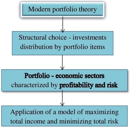
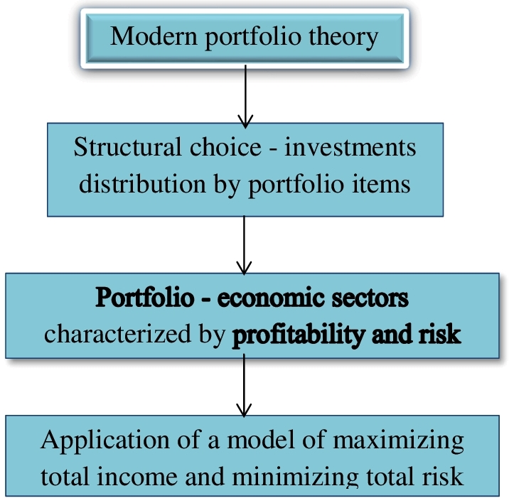
2. Research Methodology. Portfolio Theory Development

The portfolio theory can be applied to various units, not only financial ones, but also to real economic sectors, a group of which can be considered as a portfolio. Resources and investments are distributed in this portfolio, and the portfolio units are characterized by some dynamically changing value of profitability or return per unit of the invested resource and risk. The portfolio gives a certain structure for the distribution of investments by units that give a certain profitability and the risk of selling the whole portfolio. Optimization models of portfolio theory can be used to make decisions about the resources and investments distribution among portfolio items under various criteria—income maximization and risk minimization arising from portfolio units distribution. According to H. Markowitz’s efficient set theorem (Markowitz 1952, 1959), there may also be a problem of choice from a certain set of portfolios. It has already been noted that it allows choosing a certain appropriate portfolio from a set of portfolios, but the choice is limited by the criteria of either the highest income at a certain level of risk or the least risk for a certain level of income. At the level of portfolio optimization models, portfolio theory can apply them to various units in a portfolio as a quite powerful method of structural analysis. In this case, making a structural choice defined by all combinations of the specified criteria is a promising area to study. This takes the problem beyond the standard portfolio equilibrium described by J. Tobin in 1955, when he considered the choice between the stock of physical capital and money as forms of wealth that build a portfolio with the equilibrium defined by equal rates of return for all assets (Tobin 1955). According to this approach, the owner of wealth makes a choice if the least variance of the return rate does not differ the rates of income. When the rates of return are different, there is a need to diversify the portfolio in order to reduce the variance of the return rate. However, such a portfolio choice procedure does not work for the situation where the risk may also turn out to be the same, and this situation can be triggered by different investment distribution structures (Sukharev 2019, 2020a). This point is characteristic, and we can say that it is not typical for portfolio choice problem. However, structural problems in the development of the real economy can bring the situations when return and risks rates differ. More income can correlate with a greater risk, while a lower income—with less risk. There are situations when a higher income corresponds to a lower risk, and a lower income—to a greater risk. 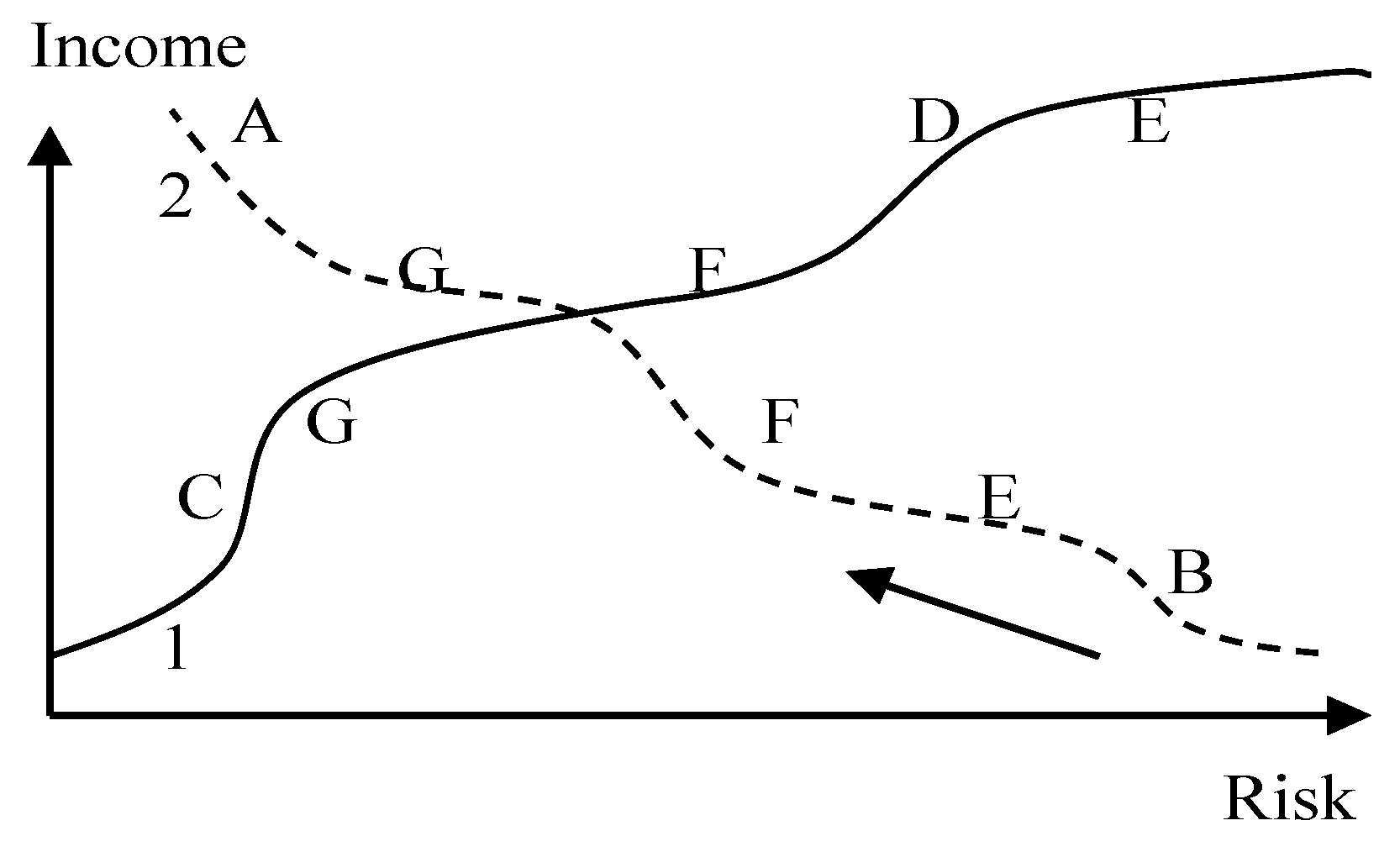Different ratios of risk and income make the choice of the distribution structure ambiguous (Figure 1). There are several economic sectors. Figure 1 shows the combination of the business risk and the profitability.

The Figure illustrates that some sectors in the economy are located along the CD line, that is, more income corresponds to a greater risk, other sectors are located along the AB line, where more income corresponds to a lower risk, and a lower income corresponds to a greater risk.

Moreover, the sectoral structure of the compared economies in different countries may correspond to the AB line or the CD line. This will mean a fundamental difference in the structural structure and functioning of the economy. A line CD denotes a structural arrangement of economic units, sectors, when greater income responds to more risk, less income—to less risk. Investments are made in activities or units with a higher risk and a higher income, which corresponds to the d-point. The units with a lower income and, therefore, lower risk, are also funded, which corresponds to the C point. This ratio does not mean that a lot is invested with a greater risk, and, even more, risk increases investments. However, the latter situation is theoretically possible, provided that the risk for other units increases at a higher rate, which may reduce the investor’s initiative. In reality, the investment will (likely) highly be distributed among the options in the area of C and D points, respectively. For the CD line, investors will make a choice between a high income and a rather significant risk to get it, or less income with the risk of earning it, then a choice arises regarding the location of the economic structure of sectors along the AB line, which is predetermined by the risk and income ratio. This is the area of A point in Figure 1. The sectors in this area will be significantly funded, since the expected return is higher there, and the risk is significantly lower than other options along this line. However, the types of activities located closer to point B will be deprived of investments, or receive them in a disproportionately smaller amount. In this case, the arrow shows a resources movement gradient between economic sectors located along the AB line from B point to A point. The choice on the CD line is determined by the perception of the income and risk rate, the investor’s inclination to risk and is ambiguous. With other things being equal, this situation does not create an investment and resource movement gradient to any part of the CD curve, but it corresponds to a more even distribution and use of resources. The AB line corresponds to a zone of resource scarcity in the economy and requires structural and institutional changes to rectify the situation. The problem of structural choice is that the risk and income ratio in the area of C and D points can be obtained from the income maximization model and distribution risk minimization model for investments and resources. Along with that, the distribution structures will differ for each model, but they will give the same risk and income combination. Then there arises the problem to choose the investment distribution structure both between C and D points, and in the vicinity of these points, if the income and risk ratio is received from different resources distributions. The assessment of the income and risk growth rate is seen to be one of the solutions for such characteristic points if different distribution structures provide different combinations of the income and risk growth rate. In this case, the distribution structure that gives the highest growth rate at the lowest risk growth rate in the vicinity of the particular characteristic point may become the results of structural choice. If income and risk growth rate cannot select the structure of the investments distribution, then one should resort to an expert assessment of the distribution under the qualitative criteria that must be separately introduced, based on the development objectives and investor preferences. As far as the distribution structures are subject to different optimization criteria, there arises the problem to choose between development options focused on the highest income or the lowest risk.

The characteristic points, similar to the Walrasian equilibrium, where demand is equal to supply, achieve equilibrium of investor behavior models, since the investor cannot choose a criterion from a previously used standard set, which requires additional criteria for making a choice.

There are three sectors E, F, G, which are located along AB and CD lines as shown in Figure 1. In addition, the structural situation changes from line 2 to line 1, that is, with approximately the same risk, the sector income E, F increase, sector G decreases. However, the economic structure is lined up along line 1, more income in the sectors corresponds to a greater risk. Therefore, curve 2 rotates and locates at the place similar to curve 1 (Figure 1).

As for sectors, we can write down the general ratio with the profitability (d) and risk (r) for each line:

(1)

we have: d_E > d_F > d_G; r_E > r_F > r_G along line 1

In other words, there is an identity in the ratio of risk and return parameters.

(2)

we have: d_E < d_F < d_G; r_E > r_F > r_G along line 2

This income and risk ratio provides the condition for the investments distribution from E sector along line 2 towards F and G sectors.

Investments movement along line 1 from G to F and to E requires an excess of the ratio of income F to G to risks, that is: d_F/d_G > r_F/r_G.

Each sector may have its own risk and return dynamics. The risk can decrease with an increase in income, then increase, or grow together with income, and then slightly decrease. An increase in risk is also possible with growth, but then a decrease in income, or in the opposite direction. There may be different options, and they are determined by the conditions of the functioning of the sector considered as a portfolio unit. The best option is associated with an increase in income and an overall risk decrease.

The analysis shows that the location of units—economic sectors along line 2 creates a problem of resource movement and sector development. It can be assumed that the structural choice of line 2 is not acceptable and requires a change in the situation, bringing it closer to line 1. It is clearly required to reduce the risk for certain sectors and to increase income. That is why the solution is to reverse line 2 to line 1.

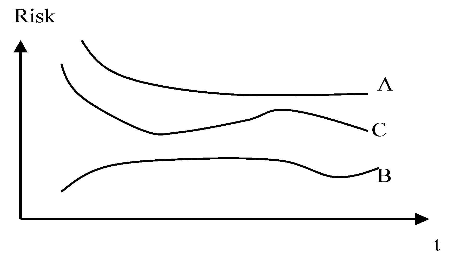
Such a move involves identifying several restructuring options, changing the ratio between the units of the analyzed portfolio with economic sectors. Sectors can move to the center, which is the intersection of lines 1 and 2, or sectors can move and increase the income with a preserved risk, or decrease the risk with a preserved income.

Figure 2 shows the possible dynamics of risk measured by the standard deviation of profit for various activities. The risk can be decreased for one type of activity, can grow in another sector (A is manufacturing, B is transactional activities, C is raw materials sector).

The portfolio can be represented by economic sectors as units with the value of their dynamically changing profitability and risk, investments allocation among the sectors. The gross product is the sectors’ gross value added; the amount of investment is the total amount of investment in the economy. In this case, the structural problem is to determine the investment distribution vector in these three sectors (generally speaking, n-types of activity can be identified similarly), which give the highest income and the lowest value of the total distribution risk. This is the structural choice problem. In some sector, the risk may increase, and then decrease. In another sector, it may decrease throughout the time interval. The resource (investment) allocation by sectors driven by the task to maximize the expected income or to minimize the total risk, affects the value of the sector’s profitability. In this case, the optimization problem becomes more complicated, since the value of the return per unit of the invested resource can change over time, it leads to dynamic optimization. It will be necessary to estimate the demand and production function depending on investments with regard to costs recalculation and to find new profitability of the unit.

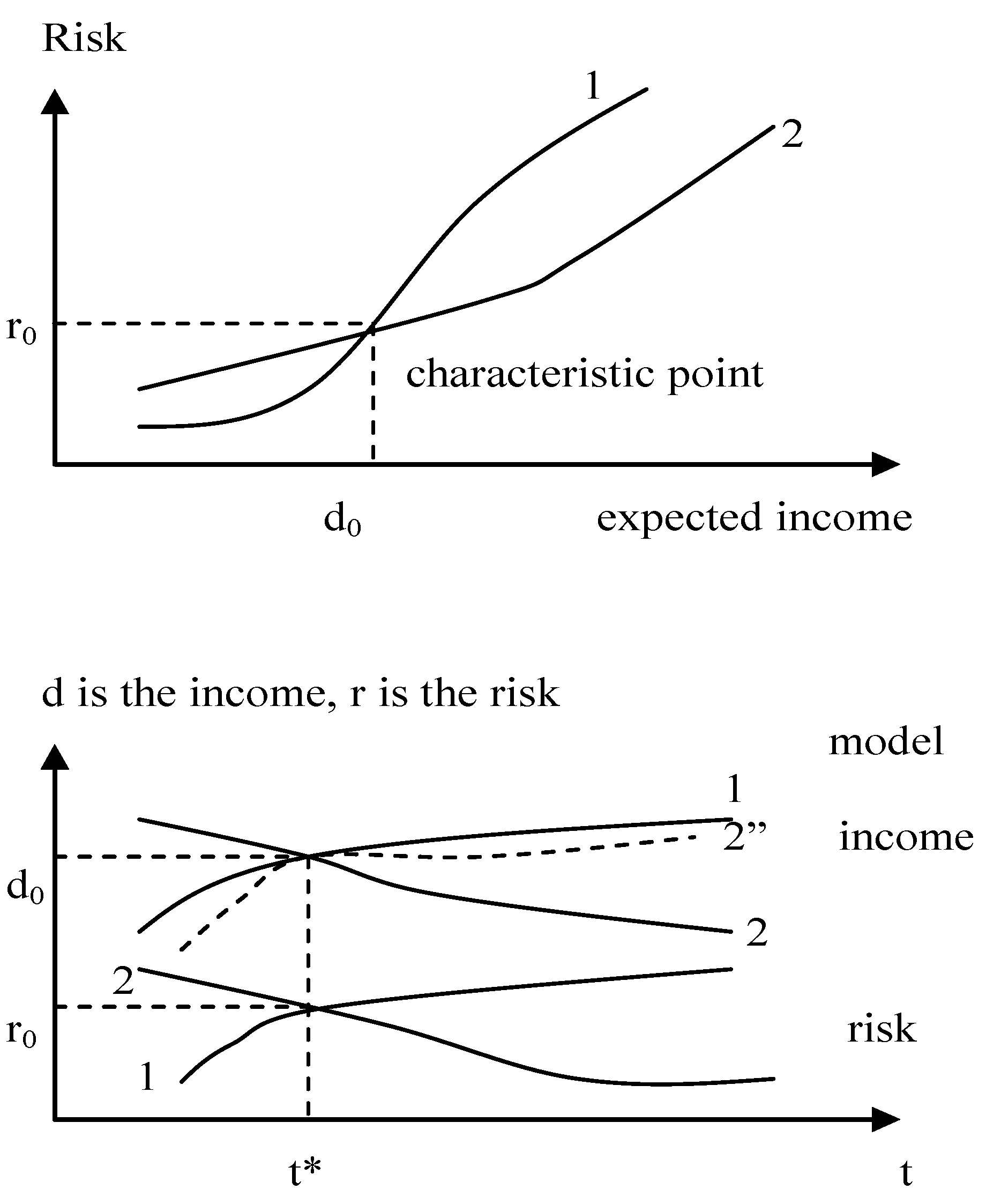
Figure 3 shows a general graph of possible changes in the expected income and risk of a portfolio under the income maximization model (1) and risk minimization model (2). According to the two models, income grows with risk. The first model shows that a higher risk corresponds to a higher income compared with the second model, where the same income gives lower risk (Figure 3, above). At the point of intersection, the ratio of income and risk arises (r₀, d₀) for two models—a characteristic point. This combination of income and risk is given by different investment distribution structures across portfolio items (sectors), which makes the structural choice ambiguous. Figure 3, below, shows time-dependent situations. The income maximization model (1) gives an increase in income and risk, while the risk minimization model gives a decrease in risk and income, however, it may happen so that the income slightly increases—line 2 (a dashed line in Figure 3, below). At t*, different distribution structures for the first and the second model give a coinciding combination of risk r₀ and income d₀.

The most reasonable choice of a portfolio structure under the efficient set theorem is up to point d₀ to the left of it along line 1, after point d₀ to the right of it—along line 2 (Figure 3, above). Thus, the options with the lowest risk are selected for a given income. However, the structural choice problem to the left or to the right of the specified income point d₀ remains important, since it is determined by the investor’s attitude to risk, investor’s aspirations regarding the amount of income.

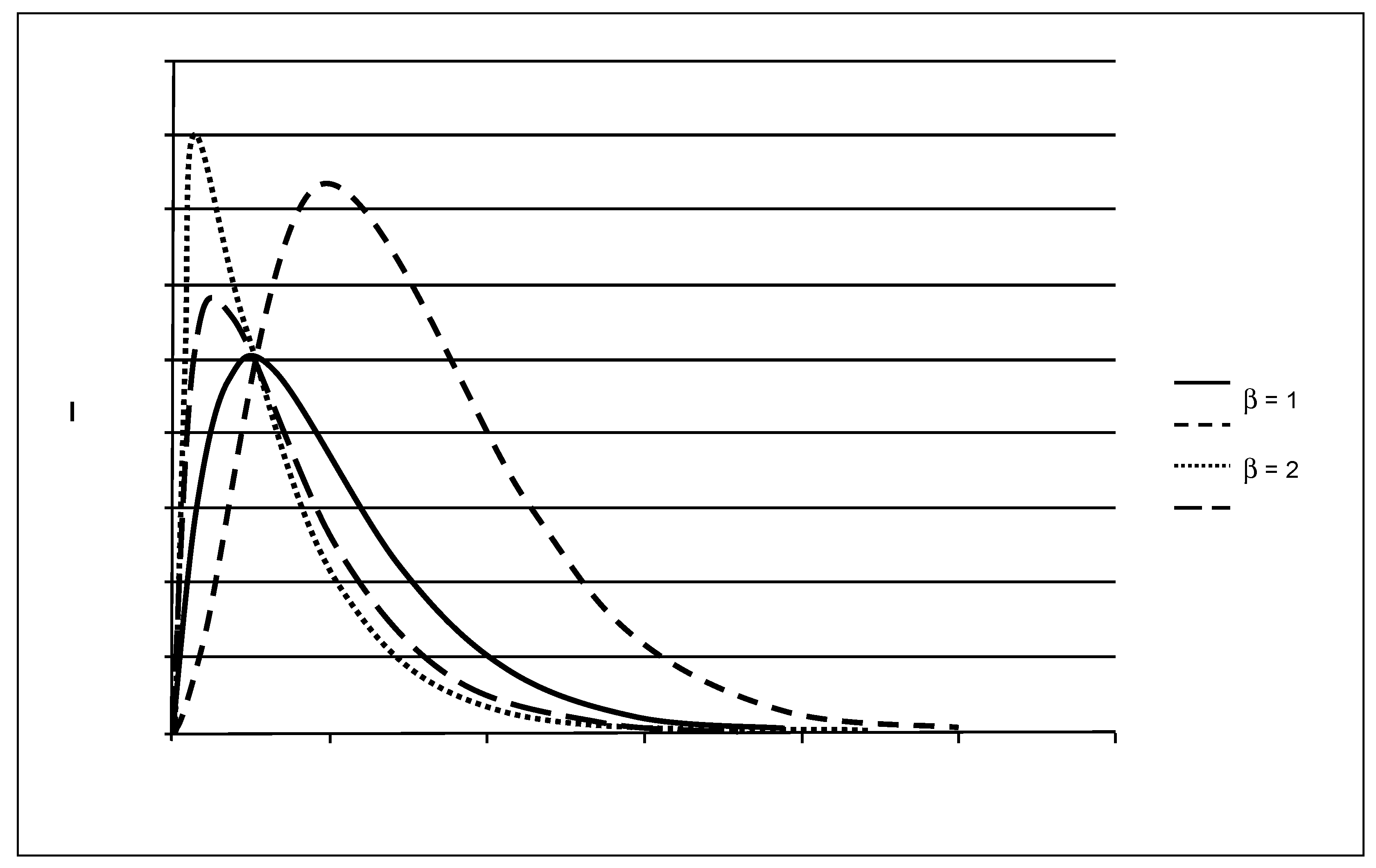
The quality of the resource (investment) will definitely impact the emerging ratio of return and risk in the sectors of the economy, as well as the initial condition of the portfolio units. The investment distribution structure is chosen with regard to the growth rate of income and risk both at characteristic points and outside them. An investment decision, whether it concerns a structure or one single unit, is risk dependent. To demonstrate this relationship, which in each case must be selected separately (for each portfolio), we will use one of the options for linking investment and risk (introduced by law). Functional analysis and a more in-depth selection of such a link, which should be carried out for characteristic units, is outside the scope of this study, but the demonstration of one possible dependency will be useful to understand the complex connections between the investments and the their risks.

To illustrate the statement, use the following model of the relationship between investments (I) in a unit (sector) and risk (r), where β is the parameter characterizing the investments sensitivity to risk. We express the model in the following formula: I = r^βe^1−r. We assume that the risk is not zero r > 0. The investment function for different β values from risk is given in Figure 4. If the investment substitution effect by risks is detected, then β < 1. Figure 4 reflects the risk dependent change in the investment function for different β values.

Figure 4 gives to the following conclusions. If the risk is low, then the smaller the β value is, the greater the investment is. With an increase in β in the low risk zone, the amount of investment (according to the introduced investment function) decreases. If the risk is higher than a certain value, the higher the β value is, the higher the investment value is.

With a small β value, investments rapidly increase with risk, and then rapidly decrease; with a further increase in risk, investments gradually decrease. After the point of intersection of the curves, for each level of risk, the value of investment is greater for a larger β.

Assuming that income can be proportional to the investment, then the risk return function repeats the investment function. In this case, the most developed economic sectors (portfolio units) will have a relatively low investment risk compared to less developed sectors, where the investment risk is higher, the amount of investment is lower, since their income (all other things being equal) is lower.

Risk aversion in this regard is higher for less developed sectors, as income is lower and the total investment will be clearly lower. Its value compared to the developed sectors is more significant. Consequently, the risk of resource loss is more unpleasant than for the developed sectors. Thus, the less well-to-do sector turns out to be discriminated, since it always has projects of lower quality (in terms of profitability and scope of activity), unlike the developed sector. This is reflected in Figure 4, where with the risk below a certain value (corresponding to the intersection point), we have a large amount of investment made by the most developed sectors of the economy, and a greater risk (to the right of the intersection point in Figure 4) gives a smaller amount of investment with a higher risk. This situation is typical for lower income, that is, for less developed sectors. They cannot provide a high amount of investment, since their income is limited. In the developed sectors, such a pattern is observed up to the maximum value of investment, and after that, the value of investment decreases with an increase in risk. We can also tolerate an increased risk aversion.

Investments I₁, I₂, …I_n can be distributed over sectors with the number n, and this distribution defines the structure choice problem. The expected income will be y₁, y₂, …y_n, respectively, expected losses are b₁, b₂, …b_n, the risk estimated here by the probability of losses is r₁,r₂, …r_n. Then the efficiency of each portfolio item will be E_i = (y_i − b_i)/I_i = y_i (1 − r_i)/I_i. The investment function I = r^βe^1−r, efficiency growth dE_i/dt > 0 serve to be the requirements for the income growth rate of each portfolio item, and this rate must exceed the risk growth rate measured by the following coefficient: β + r_i²/(1 − r_i). Or the income growth rate must exceed the risk growth rate weighted by the value r_i/(1 − r_i) plus the investment growth rate aimed at this unit. These comparisons indicate that the income growth rate and risk growth rate can be compared at a characteristic point in order to decide on an appropriate distribution structure, that is, to make a structural choice.

This analysis gives us two logical conclusions.

Firstly, the sector (portfolio object) that has restrictions at the level of income has difficulties in investing in large projects (there are restrictions at the credit and financial markets) and in making structural choices. Secondly, if the level of technological development in the sector is not high, then an option with the real technological capabilities will be selected, which will become an additional criterion for making a decision regarding the investments allocation, although in some cases a scenario associated with the expansion of these opportunities is possible. It depends on the units included in the portfolio and will determine the portfolio choice when investing.

The distribution of resources and investments among portfolio items and economic sectors can be analyzed by optimization models and methods of their numerical implementation, for example, gradient ones (Ravindran et al. 1983). Model for maximizing the total expected portfolio return and minimizing the total risk is presented below.

$$Z={\sum }_{j=1}^N{d}_j{x}_j\to max, \mathrm{with} \mathrm{restrictions}:x_j \ge 0; {\sum }_{j=1}^N{x}_j\le C$$

(1)

where:

• Z is the total expected portfolio return;
• x_j is the value of the invested resource, investment in a portfolio object, invested, for example, in the j-th sector or a type of activity;
• $d_j=\frac{1}{T}{\sum }_{t=1}^T{h}_j$ is the average return, profitability for the j-th portfolio item (sector);
• h_j is the return or profitability, the amount of income for the j-th object of the portfolio (sector) per unit of the invested resource, investment;
• T is the total time period;
• C is the volume of the invested resource, investment;
• N is the total number of portfolio items (sectors).

To minimize the aggregate portfolio risk, we use the following model:

$$R= x^{T}Qx \to \min , \mathrm{with} \mathrm{restrictions}: {\sum }_{j=1}^N{x}_j\le C, x_j \ge 0, d^{T}x \ge D$$

(2)

where Q = [ⱱ_ij²] is the covariance matrix for N portfolio units (sectors), D is the minimum average expected return, R is the total risk assessment, the value of covariance ⱱ_ij² = $\frac{1}{T}{\sum }_{t=1}^T\left(h_i\left(t\right)-d_i\right)\left(h_j\left(t\right)-d_j\right)$.

The gradient projection method is used as an optimization method for the above models in the simulations applied below (Ravindran et al. 1983; Sukharev 2019). This numerical method requires algorithmization for the optimization process of these models, the main step of which is to determine the step of descent to the surface of constraints of a nonlinear objective function that embodies the total portfolio risk.

The objective risk function R = x^TQx is as follows:

$$R = [\left(x1, x2,\dots xn\right) + \alpha \left(s^1, s^2, \dots sn\right)]Q[\left\{\begin{array}{c}{x}_1\\ x_2\\ ·\\ x_n\end{array}\right\}+\alpha \left\{\begin{array}{c}{s}^1\\ s^2\\ ·\\ s^n\end{array}\right\}]$$

(3)

where:

$$R = \left[x^{T}Q + \alpha s^{T}Q\right]\left[x + \alpha s\right] = x^{T}Qx + \alpha \left[s^{T}Qx + x^{T}Qs\right] + {\alpha }^2{s}^{T}Qs.$$

The descent step was determined by $dR/d\alpha = s^{T}Qx + x^{T}Qs + 2\alpha s^{T}Qs и d^{2}R/d{\alpha }^2 = 2s^{T}Qs$, where α is the descent step, s^j is the direction of descent (Ravindran et al. 1983). To find an extremum, the author equated the first derivative and the sign of the second derivative of the cumulative risk function over the descent step to zero. The author used an independently developed numerical optimization program.

These optimization models seem to show the problem of structural choice described above in general terms. Each optimization model is a kind of a criterion for investments allocation structure by portfolio units, regardless of the units within the portfolio. Further in the article is considered the problem of structural choice as a very promising area of research in portfolio theory.

3. Structural Choice as a Promising Task Search for Optimal Solutions in Portfolio Theory

To solve the problem of structural choice is to find the most acceptable distribution of the resource (investment) among the portfolio units, which is not reduced to any one criterion only—maximum income or minimum risk. At the same time, portfolio units are considered to be both financial assets and units of the real economy—sectors, industries, regions, etc. We apply expected income—risk approach to choose, but this should be a non-trivial approach due to a number of circumstances, which will be discussed below. Structural choice differs from portfolio choice, as the most acceptable resource distribution among portfolio units rather than a type of a portfolio is chosen, that is, a structural problem is solved. The article deals with this problem in the following calculations.

Under the income maximization model, the investments are allocated by economic sectors. Let this distribution give the expected income, which is equal to D_m. The actual distribution of investments differs from the structure in the model and gives an expected return equal to—D_f. Supposing that the expected returns are equal to D_m = D_f, but there is a difference in the structure of investment distribution. Thus, the portfolio structures are different, but they give the same return. In this case, the number of units does not change and is equal to n. Then we can write that different distribution structures i = {i1, i2, …in} and j = {j1, j2,… jn}, give income D_m =D_f, which generally does not coincide—the model and the actual structures.

Given that the structures are different, the degree of structural imperfection can be assessed, when the income in the model is higher than the actual income D_m > D_f. Here, the following coefficient is proposed:

$$S=\frac{1}{N}\sum _{j=1}^N\left|j_j-i_j\right|$$

(4)

where:

• S is the coefficient reflecting the degree of structural imperfection;
• j_j is the value of the actual resource in the portfolio unit, sector j;
• i_j is the amount of the resource in the model in sector j;
• N is the number of portfolio units, sectors.

A geometric mean weighted over N portfolio units serves to be an indicator of the structural imperfection of the portfolio (when the actual portfolio and the portfolio by the optimization model are compared). Since the absolute difference is important in this indicator, the expression in the formula (4) is taken to be a module. Such a comparison is important for identifying the deviation of the actual resource allocation by portfolio units (sectors) and the resulting model structural distribution, according to the optimization procedure. If the incomes for the model distribution and the actual distribution are nearly the same, this does not mean that the total distribution risk will be the same. If the returns are equal, the difference in risk will show how much the model solution deviates from the actual distribution.

Generally, the quantity D_m should be higher than D_f. However, it is not at all necessary for investments allocation to be guided only by the result of one or another optimization model.

If x_j is the value of the resource in the j-th unit of the portfolio, this value is in some way connected with the money supply and its change in the economy, making up the share a_jM₂, entering this sector per unit of time. Then the portfolio problem can be written as follows:

$$d_j=\frac{1}{T}{\sum }_{t=1}^T{h}_j; x_j = a_j M_2; Z\left(t\right)=M_2\left(t\right){\sum }_{j=1}^N[\frac{1}{T}{\sum }_{i=1}^T{h}_i\left(t\right)]a_j\to max$$

(5)

Thus, the portfolio optimization problem includes macroeconomic parameters and the choice between money and physical capital, which was considered to be a portfolio choice in the first works on portfolio theory. Portfolio units as sectors generate income by transforming some part of the money supply. They use cash to create a product or service with some average return d_j.

The structural problem under the portfolio theory in the given interpretation can be reduced to the definition of the vector a = {a₁, a₂, a₃, …a_N}, when the total income will be the maximum or equal to the expected income. The difference between the current distribution of money by the types of activities in the portfolio units from the model distribution indicates the need for structural changes that affect the ratio of the profitability and the risk sectors.

Let us consider the problem of portfolio optimization in the following example, where certain sectors of the economy are taken to be the units, which are given by the value of return per unit of the invested resource (

Table 1. Portfolio of five economic sectors.

Economic Sector—Portfolio Item	Profitability (Return per Unit of the Invested Resource) over Three Equal Time Intervals
1	1.0	0.7	1.2
2	0.6	0.3	–0.5
3	0.2	0.8	1.1
4	0.4	0.6	0.8
5	0.2	0.7	1.3

Source: compiled by the author.

). The resource is 100 units. In the second example, the resource is increased to 110 units. To start with, 20 resource units are allocated for each of the five sectors. The optimization goal corresponds to model (1) and (2), that is, maximizing the total income of such a portfolio and minimizing the total risk. The initial distribution for the case with an increased 110 unit resource per portfolio is accepted for the first four sectors in Table 1, 20 units each and 30 units for the fifth sector.

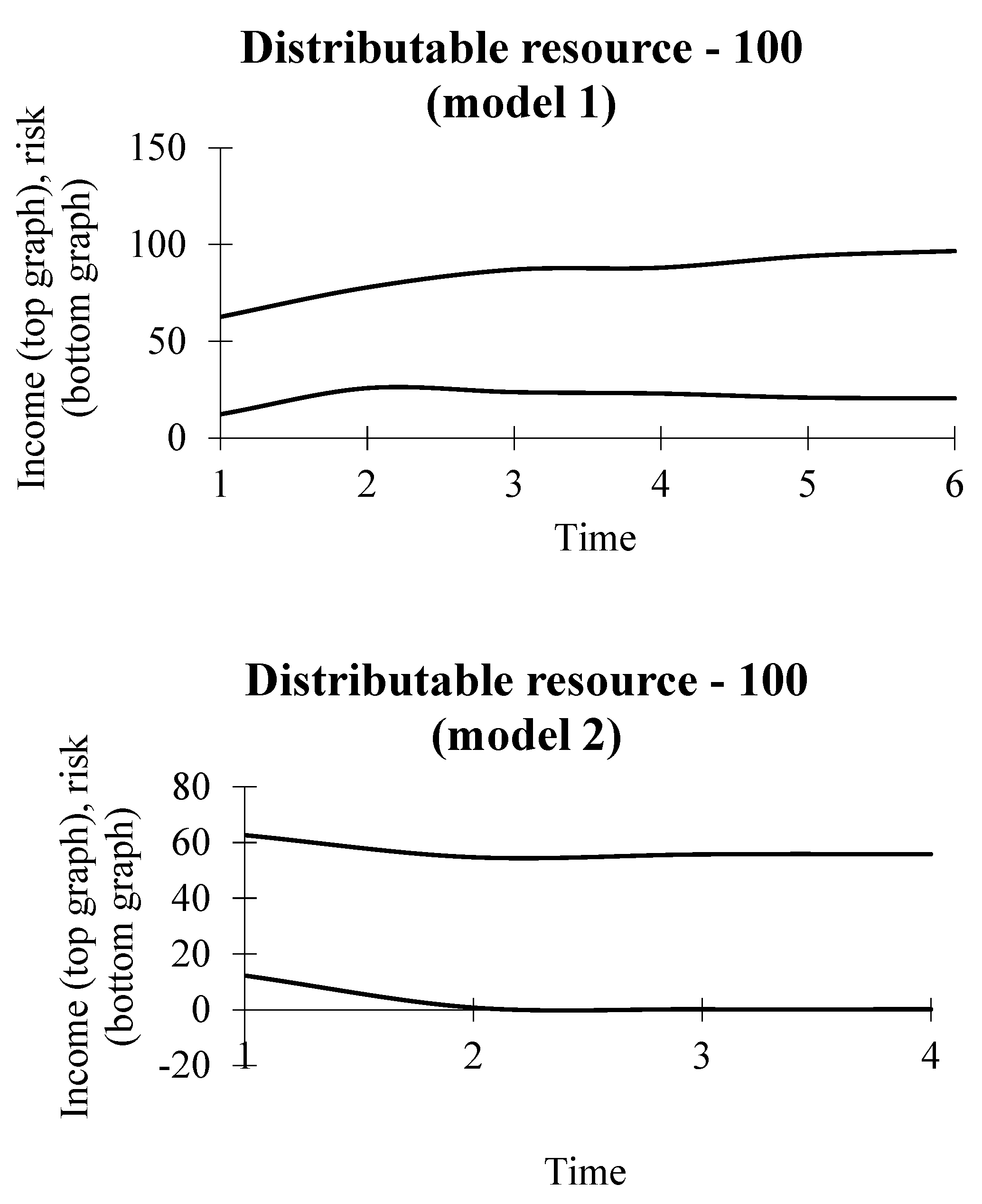
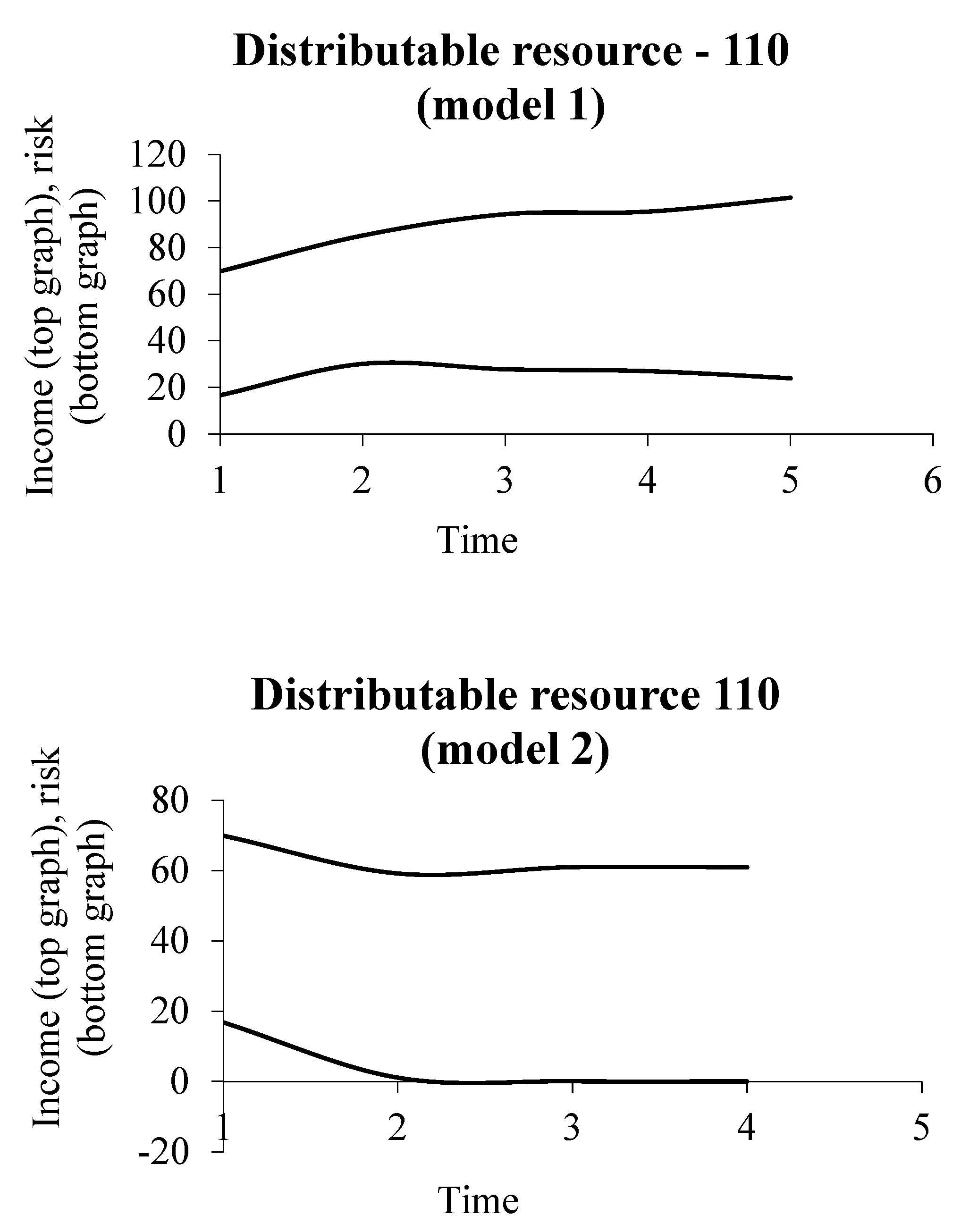
Figure 5 and Figure 6 show time dependent changes in the total income and risk of the portfolio with a resource of 100, 110 units, respectively (identical to the number of iterations of the optimization algorithm).

As can be seen from Table 1, by the third time interval, the first, third and fifth portfolio units give a return above one, that is, more than one is returned from a unit of the invested resource.

The unprofitability of the second unit will determine the distribution of investments across the portfolio, since the resource allocated to this unit will be distributed among the others. Then such a process will cover the fourth unit with a consistently low profitability. The first sector with such optimization should receive the largest resource and respond with the maximum income. Figure 5 shows that the risk is not maximized. First, it increases, then decreases and reaches the plateau. This optimization assumed that the interval profitability preserves the same dynamics as in Table 1, and the growth of the allocated resource does not lead to its change in comparison with the data in the tables. In other words, over a certain time interval, we assume that the resource change does not greatly affect the profitability2.

Figure 5, above, shows that income increases under the total portfolio income maximization model, the risk also increases, then decreases with no further income growth. It should be noted that with respect to the starting point of the even distribution of the resource, investments by sectors, the risk increases under the portfolio income maximization model, but its upward dynamics is replaced by downward dynamics (for the data specified in Table 1).

According to the risk minimization model (Figure 5, below), the risk decreases significantly with the total income. Risk minimization can lead to the fact that income does not compensate for the invested resource, an investment of 100 units. In this regard, the adequate investments allocation structure in the portfolio will follow the first model for the site, when the risk systematically decreases, but the income increases, covering the initial value of the resource. According to the risk minimization model, the smallest 0.15 risk will be with the next investment distribution {23.3; 33.34; 12.68; 18.8; 11,7} with respect to the original distribution {20; 20; 20; 20; 20}. In this case, with income maximization, the expected return is approximately 55.8 units instead of 94.0, that is, less by 40 units. At the same time, unlike the first model, the second one provides a particular resource for each type of activity, not covering the initial value of the investment. Thus, a decision requires understanding whether to increase the costs of resource allocation and to support all portfolio units, or generate costs that are not visible for the model by eliminating the resource supply to a number of units, provided current income matches investments, thereby compensating for losses from distribution investment.

With an increase in the resource to 110 units, the graphs in Figure 6, above and on the right for models 1 and 2, respectively, will shift upward. The nature of their change remains the same.

Thus, the expansion of the resource into the portfolio does not change, with the same general parameters for the portfolio units, the dynamics of its income and risk, affecting only their value upward.

Each time interval will determine the expected income and risk ratio by the structure of the resources, investments distribution. This defines the structural choice, which becomes more complicated if the number of portfolio items changes at least by one.

The article considers this situation below, and also show the structural choice in case of empirical and model (under the income maximization model) analysis of two sectors in the Russian economy (manufacturing and transactional and raw materials)3.

4. Results and Discussion

We will discuss some of most important findings from the study. The study specifies the problem of structural choice under the general approach of portfolio theory. Figure 7 and Figure 8 illustrate structural choice. The data were received from computer simulations under to the total expected portfolio return and the total risk maximization models.

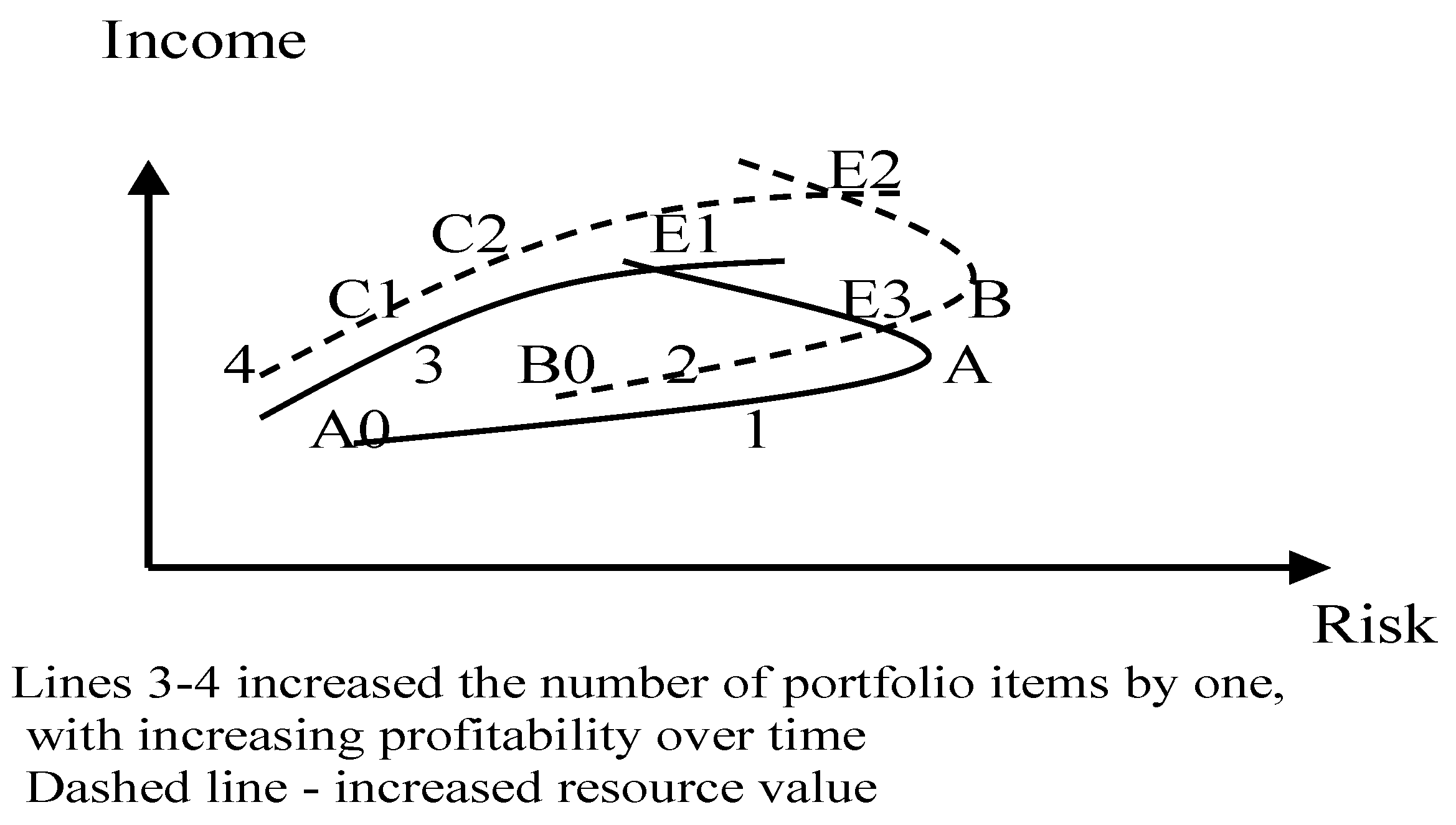
The author’s research (Sukharev 2019) on optimization models (formulas (1) and (2)) shows the changes in the income and risk ratio in a portfolio with one extra unit, when the profitability increases over a period of time together with the resource allocated to portfolio items. 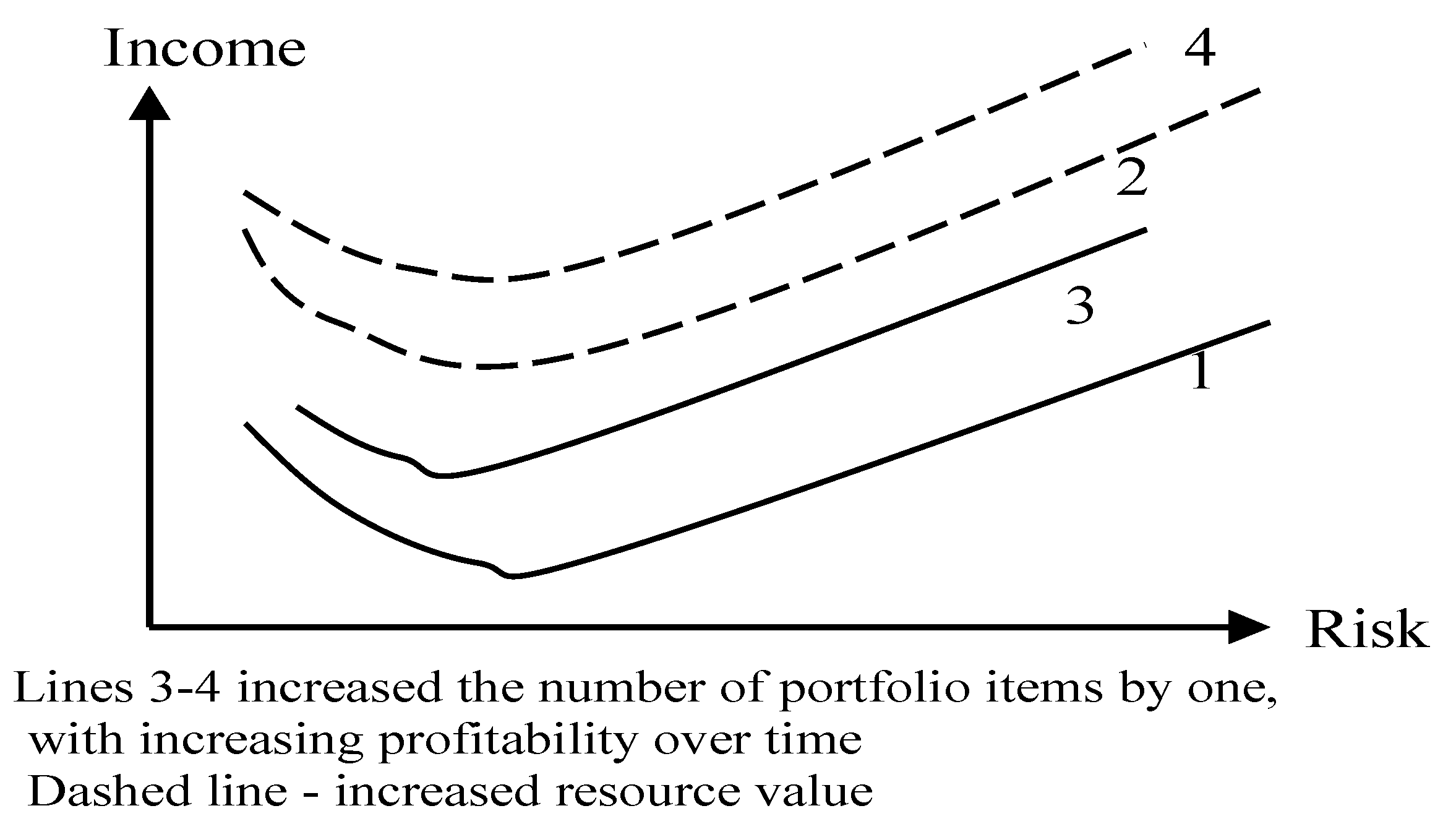The overall result will be shown here in schematic figures, reflecting the implementation of the model returns maximization (Figure 7), and risk portfolio minimization (Figure 8).

Figure 7 shows the results of optimization under the expected portfolio income maximization model (given the returns of portfolio units specified in Table 1) for the number of units n-lines 1–2 and the number of units (n + 1)-lines 3–4 (n = 5), the dashed line shows the situation with an increase in the resources allocated to the portfolio, investments, which are distributed among the portfolio units.

Several characteristic points are determined by an increase by one in the number of portfolio items rather than by the portfolio investment expansion due to the intersection of decisions obtained on the basis of not applying the model income maximization and portfolio risk minimization, as noted earlier, but due to intersecting portfolio solutions under one model—total income maximization. Point E3 is obtained on a portfolio of n-units with increasing resource (dashed line). At this point, different investment distribution structures for the same number of portfolio items give the same ratio of total return to portfolio risk. Thus, the resource for the portfolio increases, and the problem of structural choice retains its importance. According to the efficient set theorem, if total income becomes the criterion for a decision, then the line B0E3 is a choice with respect to the line A0A, since the same risk will give higher income along this line. Beyond point E3, the situation is not obvious—the same is true for points A and B, where the increase in income and risk should be compared to make a final decision. The B0E3 line gives the best decisions, and when the total risk for a given value is the criterion for their adoption, the return for this line is less risky than for the A0A line. When the resource is not increased by the portfolio, the line AE1 is a solution with respect to the line A0A of the general curve A0AE3E1 by the criterion of income, since the same risk in the upper branch gives more income. However, a comparative criterion should be chosen for different risks and different amounts of income.

Thus, the problem of structural choice is determined by the following factors: (1) simultaneous application of optimization criteria; (2) the number of portfolio items; (3) the amount of the allocated resource—an increase or decrease per portfolio. These three factors provide a combination of options for characteristic points where the structural choice is uncertain.

It should be noted that there is a structural choice for both points A and B and for any combination of points on each of the resulting curves 1–4. However, in this case, the situation is more or less solvable, since the income and risk at each point d_A, r_A, d_B, r_B do not match. In this regard, an additional criterion for making a decision can be introduced—the case when the income exceeds the risk significantly can be recognized as the most preferable for a structural choice.

Then the decision-making rule is d_A/r_A > d_B/r_B, provided this condition is fulfilled, the distribution structure of point A is accepted, otherwise it is point B.

The characteristic points E1 and E2 (Figure 7) arise from the solutions in a portfolio with a different number of units (dashed line—the number of units is increased by one). Point E2 corresponds both to an increase in the number of portfolio items and to an increase in the resource distributed among the portfolio items. Consequently, an increase in the number of portfolio units by one, as it is the case, gives the point E1 of equal total return and risk given by different portfolios and, accordingly, by the investment distribution structures over the portfolio. In this case, the decision can be made based on the preference for the number of units—the need to introduce an extra unit. If such an input is required, then it will be possible to choose a structure for point E1, but that corresponds to the solution along line 3. If the input of a unit is not necessary, then a distribution structure is chosen along line 1 at point E1. Point E2 gives portfolio structures for a small (line 2) and an increased by one (line 4) number of portfolio unit and an increased amount of investments distributed over the portfolio. Therefore, a different number of portfolio units and different resource distribution among them give the same combination of total return and portfolio risk. Moreover, both lines 2 and 4 reflect an increase in the resource per portfolio. Therefore, point E2 is higher than point E1 in terms of both income and risk. The structure can be chosen under the criterion of the presence of a unit, whether an extra object is needed or not. However, the choice between the structures E1 and E2 involves assessing the ratio of income to risk in order to understand which (for which point) structures are better under this criterion. To decide on a point, a criterion related to the need to expand portfolio items by one is required to make a final decision, already being at the right point. Comparing the sections E3E1 and the corresponding section on the segment BE2 obtained by vertical and horizontal lines drawn along the points E3E1, we can clearly see the conclusion. For the same risk, under to the efficient set theorem, the income for the area BE2 is higher, while the same income gives higher risk for this area than for E3E1. Thus, the criterion (the minimum risk or the highest income) is site dependent. This situation also shows a large uncertainty of choice, which is resolved by the ratio of income and risk for each site, although the site contains many points, but the extreme left points are acceptable for them, since they give the highest income with the lowest risk. Therefore, a number of necessary additional criteria can be added to the set efficiency theorem, thereby extending the theorem due to the examples in question and proposed solutions. It is necessary to compare the amount of income and risk in case of ambiguity of the structural choice outside the characteristic point, and also impose the condition of the highest income with the least risk. At a number of characteristic points, an additional condition will be either the number of portfolio unit, or the allocated amount of the resource, as much as required and possible to increase it. In addition, this potential increase will likely need to be weighed against the expected return and risk from portfolio disposal.

According to the efficient set theorem, the solution is line 4 with a larger dedicated resource and a larger number of portfolio units. However, the structure choice, unlike the standard portfolio choice, must answer which structure of point, C1, C2, or E2 to choose on line 4.

It should be noted that one additional portfolio item, with increasing profitability, fundamentally changed the optimization result and the dynamics of total income and risk (Figure 7, lines 3 and 4). If a smaller number of specified units give a branch of growth in the expected income and risk and a branch of income growth with a decrease in risk (lines 1 and 2), then for lines 3 and 4, the growth of income is accompanied only by an increase in risk. Thus, according to the income maximization model, various modes of income and risk dynamics are possible, depending on the combination of units and their returns. There are options when the solutions do not intersect in the considered range of dynamics (Sukharev 2019). In this case, we can compare the distance in terms of income and risk and also look at the excess of income over risk in order to make the final decision on the investment distribution structure.

As can be seen from Figure 8, the problem of risk minimization gives solutions with a decrease in income for a short interval, and then an increase in income is accompanied by an increase in risk. The smallest risk for each curve 1–4 is the left point on the chart. The lines do not show the smallest or the highest income. This raises the problem of choice between two models—income maximization, which gives the distribution of investments across the portfolio (one structure), and total risk minimization (second structure). On the ascending branches of each line, structural choice requires additional criteria, which are described in relation to Figure 7. Here they also apply. However, an increase in the resource and portfolio items requires taking into account this circumstance, although the increase in the portfolio item, as can be seen, determines the shift of the curve in Figure 8 less.

Figure 8 shows the optimal solutions for the expected return and risk of a portfolio with the same number of units as in Figure 7, but with the risk minimization model. We see identical dynamics along lines 1–4 (Figure 8); therefore, an extra unit with increasing profitability did not greatly affect the risk and its change. With the same risk, the income is higher for line 4, where the number of portfolio units and the resource (investment) allocated to the portfolio are increased. It is interesting to note that for the example under consideration, line 2 passed above line 3, that is, according to the efficient set theorem, the same risk by the criterion of income gives the best choice. This arrangement of the lines indicates the importance for the risk minimization model to increase the resource or the number of portfolio items by one (for a given value of increasing profitability). As we can see from Figure 8, line 3, where the resource is not increased, and the portfolio unit is increased by one, passes below line 2, where the portfolio resource is increased with the same number of units, as for line 1. Therefore, in this case, an increase in the volume of allocated on the resource portfolio has a determinative value and defines the structural choice according to the risk minimization model. The higher the resource is, the lower the risk for a given amount of expected income is.

It should also be noted that for a portfolio model that minimizes risk, an increase in the resource allocated to a portfolio in a situation where one unit is added to the portfolio reduces the risk gap for a portfolio with a smaller number of units by one (Sukharev 2019). With less resources allocated to the portfolio, the overall portfolio risk is higher (Figure 8). Such a result will be useful, in particular, when explaining, for example, the development of lagging countries that experience constraints on financial resources for development and a high risk of introducing innovations.

The article shows the relationship between the sectors in the Russian economy4, highlighting the manufacturing sector and the non-manufacturing sector (including transactional and raw materials activities, this sector includes transactional and raw materials—the industries are listed above in the footnote) as two portfolio items. The profitability, the risk of functioning of these sectors5 (see the results of the calculation in Figure 9 and Figure 10) assessment is shown below.

Table 2. Profit by sectors in the Russian economy, measured in 2004 rubles, million rubles6.

Sector/Years	Manufacturing	Transactional and Raw Materials
2005	994,292	2,317,654
2006	1,370,218	3,662,440
2007	1,522,453	3,217,974
2008	1,249,687	2 244,969
2009	1,052,505	2,457,857
2010	1,190,884	2,863,943
2011	1,322,514	3,248,036
2012	1,365,490	3,127,968
2013	1,270,381	3,089,964
2014	1,115,537	3,189,663
2015	1,175,053	3,435,389
2016	958,765	3,603,093
2017	1,274,235	2,865,890
2018	1,460,051	4,139,781
2019	1,666,296	3,778,306

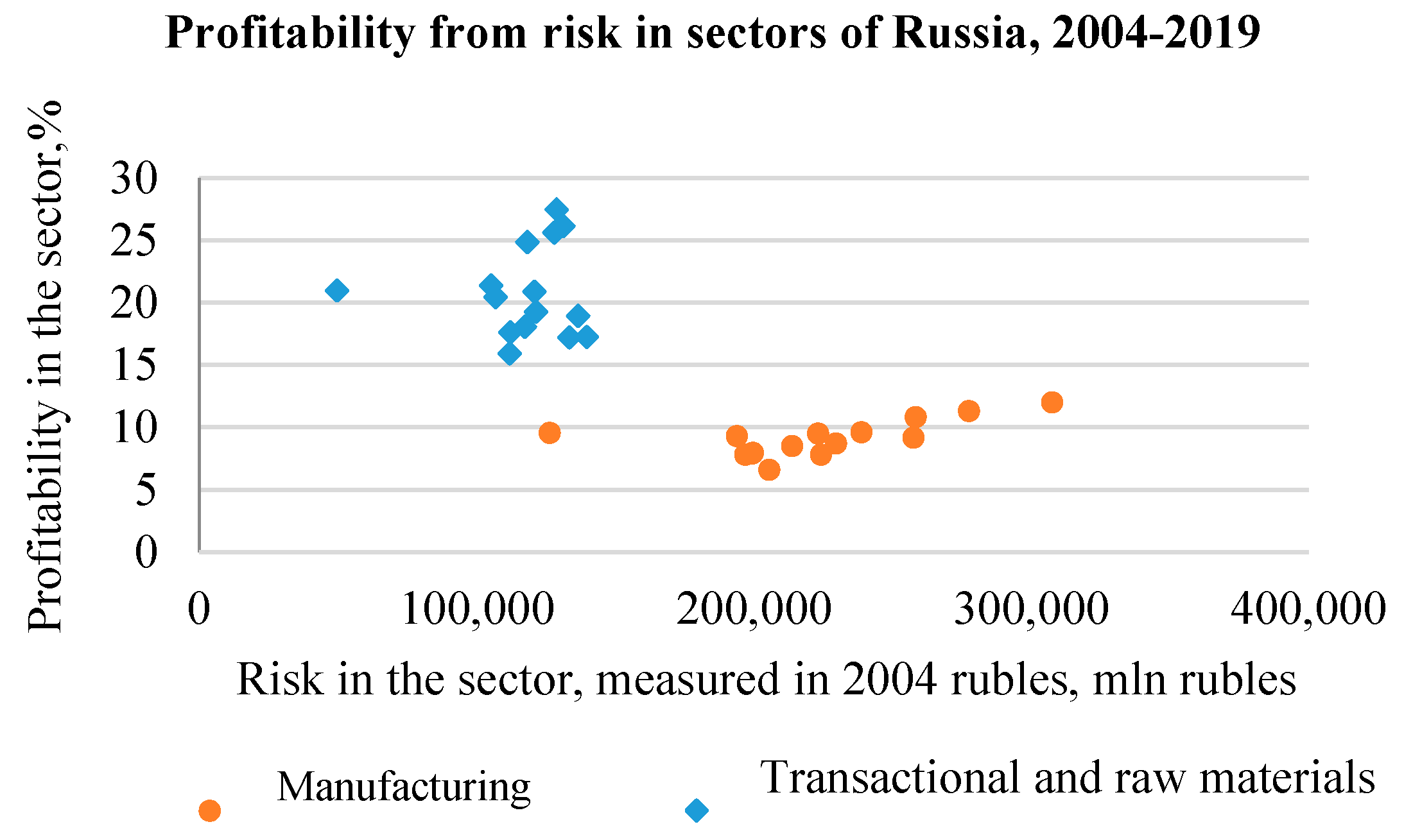
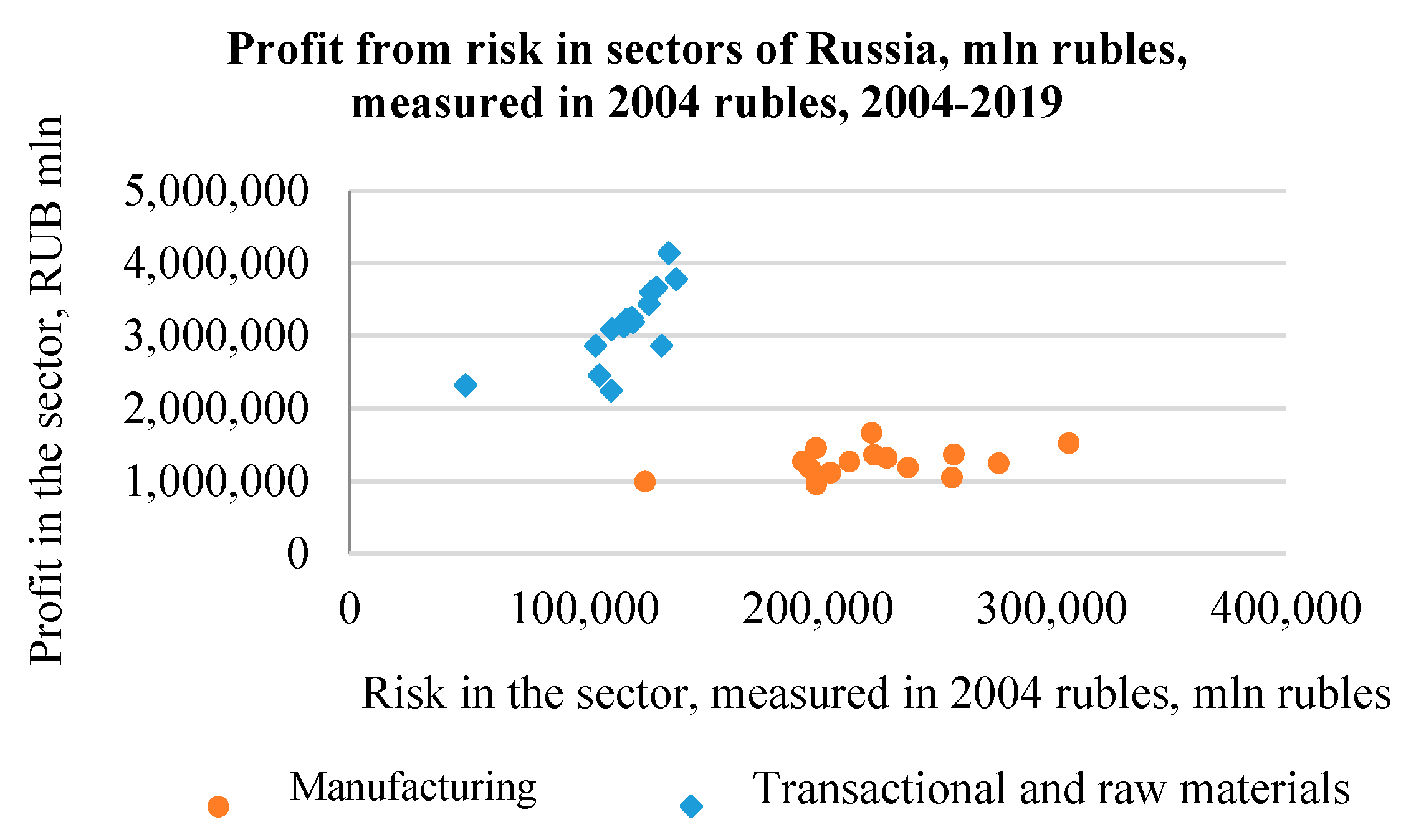
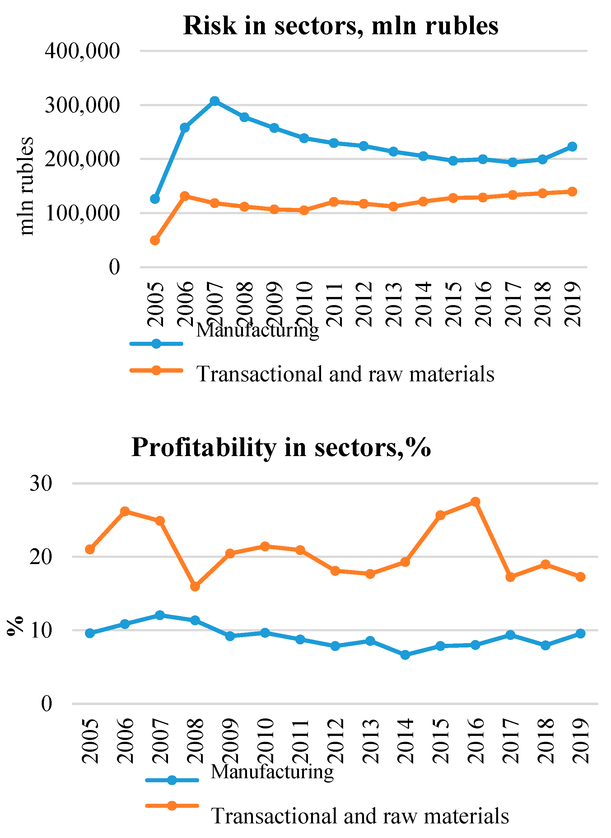
Source: compiled by the author based on Rosstat data https://www.gks.ru/compendium/document/50801.

shows profit data for the sectors in the Russian economy. The calculation was performed as follows: the amount of profit and balanced financial result, the cost of the selected sector were calculated, then the profitability was calculated, and the risk was assessed by the standard deviation of profit.

Figure 9 shows that the location of the two basic sectors in the Russian economy, considered as portfolio items, corresponds to Figure 1, the dashed line, with the manufacturing sector located at the bottom, and the transactional sector at the top. The first corresponds to high risk and low profitability (profitability), the second-to-low risk and high profitability (profitability). A similar relationship is also true for profit and risk (Figure 9, below), and an increase in risk is not accompanied by a significant increase in profit in manufacturing. An increase in profit in transactional and raw materials are accompanied by an increase in risk (the relationship is indicative of the location of the points at the top left of the graph in Figure 9, below).

Figure 10 shows that the risk decreased in manufacturing, increased in the transactional and raw materials sectors, but the ratio of risk between sectors and profitability was inverse. The profitability of manufacturing is on average 2 times lower, and the risk is much higher. Arrangement of sectors as portfolio units in Figure 1 and its dashed line creates a gradient of investment movement in favor of the sector—a unit with higher profitability and relatively low risk. Figure 11 shows the result of optimization according to the model (1) for total income maximization—the distribution of one hundred conventional units of the resource, according to the profitability of the sectors in Figure 10. Thus, real data are taken, and the model gives the structure of the distribution of the resource among sectors based on obtaining the maximum expected profit.

It follows from Figure 11 that the higher the profit is expected, the smaller the resource will be received by the manufacturing sector, and the larger the resource will be received by the transactional and raw materials sectors as portfolio units. Each rate of return (value of profit) in Figure 11 has its own distribution structure.

According to the income maximization model, the aggregate risk of such a portfolio of two sectors increases on average. The choice of resource allocation depends on the tasks facing the development of the sectors and the planned rate of return and the ratio of the expected profit and the total risk provided by the chosen structure of resource allocation and investments.

Thus, the efficient set theorem, which is the fundamental link in the portfolio theory as applied to real situations (when the portfolio units are real economic objects rather than securities or financial assets) involves the application of an extended set of criteria for structural choice and decision making. This is especially true for situations associated with the characteristic points, the number of which can be very significant. Even if the lines describing the distribution patterns do not intersect, nevertheless, the smallest distance between them simulates the characteristic point, which requires its similar resolution.

5. Conclusions

Summing up the result, it is necessary to formulate the main conclusions about the prospects for the portfolio analysis applied to both various structural problems and financial issues.

Firstly, the modern portfolio theory in its development as a separate scientific domain has deservedly acquired an independent status of a powerful tool for structural analysis and decision-making concerning the choice of investment and resource structure.

Secondly, the return and risk ratio at the initial point of the portfolio problem optimization impacts the dynamics of the investment distribution structure among portfolio units, and the implementation of a structural choice requires a comparison of income and risk for the unit. At a characteristic point, a choice will be criteria dependent, which will generate a spectrum of possible solutions and the problem of choice.

A promising area of future research is the branching of the possibilities of applying dynamic conditional optimization, with the study of various conditions impact on the target optimization functions—income to be maximized and risk to be minimized. The results already obtained from optimization models, it is possible some additional criteria or expert assessments should give a compromised option of distribution structures (although this method is not a panacea at the characteristic point, but it may have some value in practice).

Presumably, the great achievement of J. Tobin’s work was that he considered the choice between the forms of wealth (money and physical capital) and showed the possible application of portfolio theory to various units in macroeconomic analysis. In this sense, the models used here can be applied to research portfolio and broader structural choices at any level of economic organization, including the macroeconomic level, the sectoral resources distribution, and investments. Moreover, the feature of the proposed here solution is that implemented matching algorithm model maximizes income and minimizes portfolio risk by clarifying the situation in characteristic points for the structural choice.

Thus, portfolio theory should be applied to find a solution to the choice of investment distribution structures at the characteristic point, as well as to other options for the ratio of risk and expected return when comparing various portfolio structures. Moreover, the portfolios choice, composed of their real non-financial units, is associated with the fact that, together with the criterion of profitability and risk, the criterion of economic growth, described by a set of portfolio units, is fulfilled. Consequently, the author argues that the portfolio theory gives a powerful impetus to the structural analysis development by combining the classical approach of J. Tobin and H. Markowitz (Tobin 1955; Markowitz 1959) and its modern interpretation by their followers, which gives a tangible prospect of such an extended application of portfolio theory, especially in the solution of structural choice problem.