A Machine Learning Integrated Portfolio Rebalance Framework with Risk-Aversion Adjustment

Abstract

We propose a portfolio rebalance framework that integrates machine learning models into the mean-risk portfolios in multi-period settings with risk-aversion adjustment. In each period, the risk-aversion coefficient is adjusted automatically according to market trend movements predicted by machine learning models. We employ Gini’s Mean Difference (GMD) to specify the risk of a portfolio and use a set of technical indicators generated from a market index (e.g., S&P 500 index) to feed the machine learning models to predict market movements. Using a rolling-horizon approach, we conduct a series of computational tests with real financial data to evaluate the performance of the machine learning integrated portfolio rebalance framework. The empirical results show that the XGBoost model provides the best prediction of market movement, while the proposed portfolio rebalance strategy generates portfolios with superior out-of-sample performances in terms of average returns, time-series cumulative returns, and annualized returns compared to the benchmarks.

1. Introduction

The purpose of financial portfolio optimization is to allocate the capital weights among a set of assets in an optimal manner such that the investor’s utility is maximized. The earliest study in the portfolio optimization field dates back to the 1950’s with the mean-variance model proposed by Markowitz (1952), which seeks the optimal trade-off between the reward and risk measures represented by the mean and the variance of the portfolio returns. Though the mean-variance model is widely used in practice, it has two main well-known limitations. The solution of the mean-variance model is consistent with the principle of utility maximization only if the asset returns are normally distributed or the utility function is quadratic, where the normality and quadraticity are not usually satisfied in the real financial world. To mitigate the shortcomings of the variance, many other risk measures have been investigated, which include but are not limited to the semi-variance (Markowitz 1959; Markowitz et al. 1993), semi-deviation Ogryczak and Ruszczyński (1999, 2001), mean absolute difference (Konno and Yamazaki 1991), Value-at-Risk (Duffie and Pan 1997; Gaivoronski and Pflug 2004), Conditional-Value-at-Risk (CVaR) (Rockafellar and Uryasev 2000), Entropic Value-at-Risk (EVaR) (Ahmadi-Javid 2012), and Gini’s Mean Difference (Shalit and Yitzhaki 1984; Yitzhaki 1982). We refer to Fabozzi et al. (2010) for a detailed review of risk measures. Each of the risk measures employed in the portfolio optimization framework constitutes a family of mean-risk models.

The efficient solutions of the bi-objective mean-risk portfolios can typically be achieved by solving one of the three optimization models: (1) maximizing the expected return subject to an upper-bounded budget level on the risk measure; (2) minimizing the risk measure while requiring the mean return to exceed an acceptable threshold value; (3) maximizing the risk-adjusted mean return, which takes the form of mean return less the risk measure multiplied by a risk-aversion coefficient selected by the investor. This risk-aversion coefficient represents the preference or risk attitude of the investor toward the market environment, which is a reflection of the market trend. If the market is in a bearish trend, the investor is supposed to be more risk-averse and adjust the portfolio to reduce risk, which can be achieved by solving the model with a large risk-aversion coefficient value. In contrast, if the market is in a bullish trend, the investor should be less risk-averse and adjust the portfolio with more attention to gain return, which leads to a smaller value of the risk-aversion coefficient. In real-world financial industries with a multi-period investment horizon, to accommodate the volatile market environment, the portfolio is constructed within a dynamic rebalance strategy to obtain high overall returns while keeping the risk under control (Geweke and Amisano 2010). If the market trends can be well captured and predicted, the investors can rebalance their portfolios by simply adjusting the risk-aversion coefficient. The adjustment of the risk-aversion coefficient in response to the (predicted) market trend thus plays a critical role in this portfolio rebalance strategy. We propose to address this adjustment via machine learning models utilizing the technical indicators.

Machine learning algorithms are widely used to forecast the direction of stock markets. For instance, Ni et al. (2011) build a predictive model that combines the fractal feature selection method and support vector machine to predict the daily price moving direction of an index. Hu et al. (2018) integrated the sine-cosine algorithm and the basis of back propagation neural networks to predict the directions of the S&P 500 and Dow Jones Industrial Average Indices. García et al. (2018b) used a hybrid fuzzy neural network to predict the next day direction of the German DAX-30 stock index. Cervelló-Royo and Guijarro (2020) compared the accuracy of four different machine learning techniques (Random Forest, Deep Learning, Gradient Boosting Machines, and Generalized Linear Models) for the 10-days ahead trend of NASDAQ index prediction.

The technical indicators are computed based on historical data (e.g., past price and volume patterns) of one specific asset to derive useful information that is believed to persist into the future. Schwager (1993, 1995) finds that technical analysis is used by many top traders and fund managers through his interviews and conversations. Covel (2004, 2009) advocates for the use of technical analysis exclusively by analyzing various practical and successful case studies in hedge fund companies. The technical indicators are devised to assist the trading actions by sending trading signals (i.e., buy or sell signals) to the analysts for the classical all-or-nothing trading strategy. The profitability of asset trading rules based on technical analysis, such as filter rules Fama and Blume (1966), moving averages Brock et al. (1992); Kwon and Kish (2002), momentum Ahn et al. (2003); Conrad and Kaul (1998), and automated pattern recognition Lo et al. (2000) have been well studied in the literature. The power of the technical analysis was later extended to the asset allocation and portfolio optimization problems. By assuming a log-utility function of the investor, Zhu et al. (2009) considers an asset allocation model with two assets (i.e., one risky and one risk-free) by incorporating the trading signals generated by technical indicators on the specification and adjustment of the risk tolerance coefficient in the utility function. Their numerical results display the superior performance of the proposed approach compared to the all-or-nothing rule as a benchmark. Gorgulho et al. (2011) investigate the financial portfolio management strategies by taking advantage of technical indicators such as moving averages and relative strength indicator, and demonstrate its profitability over the classical buy-and-hold and purely random strategies. Ji et al. (2017a) employ the moving averages to detect persisting market trend movements and to generate buy-hold-sell signals that assist investors in adjusting their portfolio allocations.

The studies above utilize historical information and technical indicators to detect and describe the market trend up to date. However, no prediction of the market trend into the future has been embedded into the portfolio optimization model or the portfolio rebalance strategy. In the era of big data, machine learning and artificial intelligence techniques, such as neural network, linear and logistic regression models, and random forest, have been widely and deeply applied in the financial industry for price forecasting, market pattern recognition, and movement prediction. An excellent survey paper by Thawornwong and Enke (2004) reviews different neural network approaches used in 45 journal articles for stock returns forecasting. Chen et al. (2008) propose a dynamic proportion portfolio insurance (DPPI) strategy based on the popular constant proportion portfolio insurance (CPPI) strategy. The constant multiplier in CPPI is generally regarded as the risk multiplier. Since the market changes constantly, we think that the risk multiplier should change according to market conditions. This research identifies risk variables related to market conditions. Ko and Lin (2008) introduce a resource allocation neural network model to optimize the investment weight of a portfolio. This model will dynamically adjust the investment weight as a basis of $100\%$ of the sum of all of the asset weights in the portfolio. The experimental results demonstrate the feasibility of optimal investment weights and the superiority of ROI of the buy-and-hold trading strategy compared with the benchmark Taiwan Stock Exchange (TSE). Freitas et al. (2009) present a new prediction-based portfolio optimization model that can capture short-term investment opportunities, which utilizes the neural network to predict stock returns and derive a risk measure based on the prediction errors. Chen et al. (2010) describe a decision-making model of dynamic portfolio optimization for adapting to the change in stock prices based on an evolutionary computation method known as genetic network programming (GNP). The proposed model, making use of the information from technical indices and candlestick chart, is trained to generate portfolio investment advice. Within the framework of Bayesian analysis, Zhou et al. (2014) construct portfolios with out-of-sample return forecasting based on the latent threshold dynamic models by considering the dependencies among the sparse factors.

In a more recent study, Ji et al. (2019) propose a multi-period dynamic portfolio optimization framework that allows the investor to adjust his or her risk attitude (i.e., risk-aversion coefficient) by fusing the market trend movement information predicted by machine learning models using a set of technical indicators as the input features. The proposed framework consists of two steps: first, a set of technical indicators (e.g., moving averages, momentum, relative strength index) generated from a market index (e.g., S&P 500) will feed the machine learning classification models (e.g., logistic regression, support vector machines) to predict the market movement (e.g., going up or down). Secondly, by adjusting the risk-aversion coefficient according to the predicted market movement, the investor will solve a mean-risk portfolio optimization model to obtain the portfolio weights and carry the portfolio into the next period. They employ Gini’s Mean Difference as the risk measure in the portfolio optimization. Our paper is an extension of the work by Ji et al. (2019), with significant improvements from the following three perspectives:

• More flexible selection of the risk-aversion coefficient. In Ji et al. (2019), they assume that the risk-aversion coefficient is selected from a finite and ordered set that is pre-determined by the investor. The selection of the risk-aversion coefficient is limited within this prescribed set and is only allowed to change according to its adjacent values. In this study, we modify the objective function of the mean-risk optimization model into a normalized version, so that the predicted probability of market movement from the machine learning models can be directly incorporated as an input of the risk-aversion coefficient, which alleviates the complication of specifying a prescribed set.
• More technical indicators are used to train the machine learning models.Ji et al. (2019) employ 9 different technical indicators to feed the machine learning classification models, while we will consider an extensive set of 14 technical indicators with a total of 37 features or predictors generated by the different parametric settings of those indicators.
• More comprehensive empirical tests are conducted to derive numerical insights. Using the rolling-horizon approach, Ji et al. (2019) conduct numerical tests with a horizon of 156 periods (3 years), with 104 periods in each rolling-window for in-sample training and portfolio optimization, and 52 periods (1 year) for out-of-sample performance evaluation. In this study, we carry out the empirical tests with a longer horizon of 1252 periods (24 years from 1995 to 2018), with 260 periods (5 years) in each rolling-window and 992 periods (19 years) for the out-of-sample performance evaluations.

The remainder of this paper is organized as follows. Section 2 introduces the Mean-Gini model using Gini’s Mean Difference as the risk measure, the employed technical indicators and machine learning classification models. The machine learning integrated portfolio rebalance framework is established in Section 3. The results of empirical studies are reported in Section 4. Section 5 concludes the paper.

2. Preliminaries

To be self-contained, we will revisit the three key parts to establish the machine learning integrated portfolio rebalance framework. Section 2.1 reviews the Gini’s Mean Difference (GMD) and Mean-Gini portfolio model. Section 2.2 illustrates the 14 technical indicators employed in our study. Section 2.3 briefly introduces two machine learning approaches, that is, logistic regression (LR) and extreme gradient boosting (XGBoost).

2.1. Gini’s Mean Difference and Mean-Gini Model

We first revisit the Mean-Gini portfolio optimization model, which employs a portfolio’s mean return as the reward measure and Gini’s Mean Difference (GMD) as the risk measure. Yitzhaki (1982) firstly proposed adopting Gini’s Mean Difference as a risk measure in portfolio analysis. Numerous studies have been contributed to the literature following the stem; see Yitzhaki (1983); Shalit and Yitzhaki (1984); Ringuest et al. (2004); Ji et al. (2017b); Ji et al. (2018); Shalit and Greenberg (2013); Sehgal and Mehra (2017) for examples. We are motivated to use GMD for three main merits: (i) GMD is demonstrated to be consistent with second-order stochastic dominance and is a coherent measure of risk (see Artzner et al. 1999); (ii) in contrast to variance, GMD does not require the normality assumption of asset returns nor the quadratic utility function of the investor; and (iii) GMD provides diversity of the constructed portfolios, which is in agreement with the Basel II Accord recommendations (Basel Committee on Banking Supervision 2004).

Let us first introduce some notations before stepping into the mathematical definitions. We denote by J the total number of periods of historical data, and let I be the total number of candidate assets/stocks to be considered to construct portfolios. Our decision variable, $w_i,i=1,\dots ,I$, represents the capital weights (i.e., percentage of the capital) invested in asset i. Let $r_{ij}$ denote the historical return of asset i in period j, $i=1,\dots ,I$ and $j=1,\dots ,J$. The mean return of asset i is denoted by ${\mu }_i$.

With the above notations, we thus can compute the portfolio return $R_j$ in period $j,j=1,\dots ,J$, and the mean return of the portfolio R as follows:

$$\begin{array}{c}\hfill R_j=\sum _{i=1}^I{r}_{ij}{w}_i\end{array}$$

(1)

$$\begin{array}{c}\hfill R=\sum _{i=1}^I{\mu }_i{w}_i.\end{array}$$

(2)

The Gini’s Mean Difference (GMD) is defined as one half of the mean absolute difference between all pairs of realizations of the portfolio return Yitzhaki (1982). We let the Gini’s Mean Difference be denoted by G, and it can be formally formulated as follows:

$$\begin{array}{c}\hfill G=\frac{1}{J(J-1)}\sum _{j=1}^{J-1}\sum _{j^{\prime }>j}^J|R_j-R_{j^{\prime }}|=\frac{1}{J(J-1)}\sum _{j=1}^{J-1}\sum _{j^{\prime }>j}^J|\sum _{i=1}^I{w}_i(r_{ij}-r_{i{j}^{\prime }})|.\end{array}$$

(3)

Employing the mean return (R) as the reward measure and the GMD (G) as the risk measure, the Mean-Gini model can be formulated in the form of maximizing the risk-adjusted mean return.

$$\begin{array}{cc}\hfill max& R-\alpha G\hfill \end{array}$$

(4)

$$\begin{array}{cc}\hfill \mathrm{s}.\mathrm{t}.& R=\sum _{i=1}^I{\mu }_i{w}_i,\hfill \end{array}$$

(5)

$$\begin{array}{cc}\hfill & G=\frac{1}{J(J-1)}\sum _{j=1}^J\sum _{j^{\prime }\ne j}^J{R}_{j{j}^{\prime }},\hfill \end{array}$$

(6)

$$\begin{array}{ccc}\hfill & R_{j{j}^{\prime }}\ge R_j-R_{j^{\prime }},\hfill & \hfill j,j^{\prime }=1,\dots ,J;j\ne j^{\prime }\end{array}$$

(7)

$$\begin{array}{ccc}\hfill & R_{j{j}^{\prime }}\ge 0,\hfill & \hfill j,j^{\prime }=1,\dots ,J;j\ne j^{\prime }\end{array}$$

(8)

$$\begin{array}{cc}\hfill & \sum _{i=1}^I{w}_i=1,\hfill \end{array}$$

(9)

$$\begin{array}{ccc}\hfill & w_i\ge 0,\hfill & \hfill i=1,\dots ,N.\end{array}$$

(10)

In the objective function (4), $\alpha \ge 0$ is a user-defined risk-aversion coefficient representing the attitude of the investor toward the risk. Constraints (6) to (8) linearize the GMD expression (3) by introducing auxiliary non-negative variables $R_{j{j}^{\prime }}$ that represent the positive difference between the pair of portfolio realizations, that is, $R_{j{j}^{\prime }}=max\{R_j-R_{j^{\prime }},0\},j,j^{\prime }=1,\dots ,J;j\ne j^{\prime }$. Constraint (9) enforces all available capital to be invested in the portfolio. Constraint (10) prevents short selling.

In the above Mean-Gini model, the risk-aversion coefficient $\alpha$ is a predefined parameter input, seeking a trade-off between two objectives (maximizing the expected return R and minimizing the risk G), by imposing a penalty on the risk. By solving the above model with various $\alpha$ value, one can trace out the Mean-Gini efficient frontier of the portfolios. In a multi-period setting with portfolio rebalance strategy, the risk-aversion coefficient should be adjusted according to the risk attitude of the investor which is heavily steered by the market trend movements. That is, when the market is going up, the investor is less risk-averse (or even risk-seeking), thus looking for higher returns by setting a small value on the coefficient $\alpha$; whereas if the market is going down, then the investor becomes more risk-averse, thus aiming to reduce risk by adjusting the coefficient $\alpha$ to a large value.

The selection of the risk-aversion coefficient $\alpha$ is arbitrary. To provide an unbiased assessment, it is critical to ensure that this coefficient has a similar impact on the mean return and GMD objectives. We thus transform the original objective function (4) into a normalized version. The normalized Mean-Gini (NMG) model reads:

$$\begin{array}{cc}\hfill \mathbf{NMG}:max& \lambda \frac{R-R_{min}}{R_{max}-R_{min}}-(1-\lambda )\frac{G-G_{min}}{G_{max}-G_{min}}\hfill \\ \hfill s.t.& \left(5\right)-\left(10\right),\hfill \end{array}$$

(11)

where R and G represents the expected return and Gini’s Mean Difference of the constructed portfolio, respectively. $G_{min}$ denotes the minimal GMD, which can be obtained by minimizing GMD as a single objective without constraints imposed on expected return. $R_{min}$ denotes the minimal expected return corresponding to the portfolio with $G_{min}$. $R_{max}$ and $G_{max}$ represent the maximal expected return and GMD when solving the model with the single objective of maximizing the expected return with no restrictions on the risk measure GMD. After the min-max normalization, the two terms $\frac{R-R_{min}}{R_{max}-R_{min}}$ and $\frac{G-G_{min}}{G_{max}-G_{min}}$ will range from 0 to 1. In addition, we use the weighted coefficient $\lambda$ and $1-\lambda$ associated with the return and risk objectives, respectively, where $\lambda \in [0,1]$ is a user-defined parameter representing the probability of the market going up. When $\lambda =1$, that is, the probability of the market going up is 1, then the NMG model reduces to the form of maximizing the expected return solely, which reflects the risk-seeking attitude of the investor during an upward trend. When $\lambda =0$, that is, the probability of the market going down is 1, then the NMG model is equivalent to minimizing the risk measure GMD, which captures the risk-averse preference during a downward trend. By adopting the risk-aversion coefficient $\lambda$ with a probability interpretation, it allows us to integrate this (predicted) probability obtained by machine learning classification models for predicting the movement of the market.

2.2. Technical Indicators

We use a set of technical indicators generated from a market index as the predictors or features in order to build the machine learning classification models for market movement. A market index, such as Standard & Poor’s 500 (S&P500) and Dow Jones Industrial Average (DJIA), is generally developed to measure the weighted value of a section of the stock market, thus intuitively a reliable indicator representing the market trend. The task of the machine learning models is to predict the movement (i.e., up or down) of the market via a set of technical indicators that are related to the past values and volume pattern of a market index. There are hundreds of technical indicators available with various definitions to capture different information. We refer the interested readers to Colby (2002) for more comprehensive descriptions for the technical indicators. Here, we only introduce briefly the 14 popular and widely used indicators adopted in the machine learning models within our study, including Simple Moving Average (SMA), Weighted Moving Average (WMA), Exponential Moving Average (EMA), Moving Average Convergence/Divergence (MACD), Relative Strength Index (RSI), Average Directional Movement Index (ADX), Commodity Channel Index (CCI), Stochastic Momentum Index (SMI), Ease of Movement (EMV), Money Flow Index (MFI), Chaikin Money Flow (CMF), Volume-weighed Average Price (VWAP), Bollinger Bands (BBands), Parabolic Stop-and-Reverse (SAR).

The above 14 technical indicators are widely used both in the academia and the finance industry. Each of them is equipped with different parameters. To keep the paper succinct as well as self-contained, we provide a brief description of each technical indicator in Appendix A with

Table A1. Computing Equations of Technical Indicators.

Technical Indicators	Equation
SMA	$\frac{1}{n}{\displaystyle \sum _{i=0}^{n-1}}{P}_{M-i}$
WMA	$\frac{{\displaystyle \sum _{i=0}^{n-1}}(n-i)P_{M-i}}{{\displaystyle \sum _{i=0}^{n-1}}n-i}$
EMA	${\displaystyle \sum _{i=0}^{n-1}}\left[\alpha {(1-\alpha )}^i{P}_{M-i}\right]$, $\alpha =2/(n+1)$
MACD	$DIF=EMA(close,n_1)-EMA(close,n_2)$
	$MACD=EMA(DIF,n_3)$
RSI	$100-\left[\frac{100}{1+\frac{EMA(U,n)}{EMA(D,n)}}\right]$, U & D: upward and downward movements
ADX	$+DI=100\times SMA(+DM,n)$, $+DM$: positive directional movement
	$-DI=100\times SMA(-DM,n)$, $-DM$: negative directional movement
	$DX=\left|\frac{[+DI]-[-DI]}{[+DI]+[-DI]}\right|$
	$ADX=SMA(DX,n)$
CCI	$\frac{1}{0.015}·\frac{P_M-SMA\left(P_M\right)}{MD\left(P_M\right)}$, $MD$: mean absolute deviation
SMI	$c=max\{P_M^{high},\dots ,P_{M-(n-1)}^{high}\}+min\{P_M^{low},\dots ,P_{M-(n-1)}^{low})\}$
	$cm=P^{close}-\frac{1}{2}·c$
	$c{m}_1=cm·n_1·EM{A}_{n_1}$, $n_1$: number of periods for initial smoothing
	$c{m}_2=c{m}_1·n_1·EM{A}_{n_1}$
	$hl=max\{P_M^{high},\dots ,P_{M-(n-1)}^{high}\}-min\{P_M^{low},\dots ,P_{M-(n-1)}^{low})\}$
	$h{l}_1=hl·n_2·EM{A}_{n_2}$, $n_2$: number of periods for double smoothing
	$h{l}_2=h{l}_1·n_2·EM{A}_{n_2}$
	$SMI=100\times \left(\frac{c{m}_2}{h{l}_2/2}\right)$
EMV	$MidpointMove=\frac{P^{high}-P^{low}}{2}-\frac{P_{-1}^{high}-P_{-1}^{low}}{2}$
	$BoxRatio=\frac{Volume/10000}{P^{high}-P^{low}}$
	$EMV=\frac{MidpointMove}{BoxRatio}$
MFI	$P=\frac{P^{high}+P^{low}+P^{close}}{3}$
	$RawMoneyFlow=P\times Volume$
	$MoneyFlowRatio=\frac{n-periodPositiveMoneyFlow}{n-periodNegativeMoneyFlow}$
	$MFI=100-\frac{100}{1+MoneyFlowRatio}$
CMF	$MoneyFlowMultiplier=\frac{(P^{close}-P^{low})-(P^{high}-P^{close})}{P^{high}-P^{close}}$
	$MoneyFlowVolume=MoneyFlowMultiplier\times Volume$
	$CMF=\frac{{\sum }_1^{n}MoneyFlowVolume}{{\sum }_1^{n}Volume}$
VWAP	$\frac{{\displaystyle \sum _{i=0}^{n-1}}volum{e}_{M-i}\times P_{M-i}}{{\displaystyle \sum _{i=0}^{n-1}}volum{e}_{M-i}}$
BBands	$P=\frac{P^{high}+P^{low}+P^{close}}{3}$
	$MidBand=SMA\left(P\right)$
	$UpperBand=MidBand+F\times \sigma \left(P\right)$, $\sigma \left(P\right)$: standard deviation of P
	$LowerBand=MidBand-F\times \sigma \left(P\right)$
SAR	$RSAR=PriorSAR+PriorAF\times (PriorEP-PriorSAR)$, $AF$: Acceleration Factor
	$FSAR=PriorSAR-PriorAF\times (PriorSAR-PriorEP)$, $EP$: Extreme Points

summarizing the equations to compute them. Using different parameter settings, we create a total of 37 versions of different indicators, which are adopted as predictors (or called features) to train the classification models, with the target to predict the movement (i.e., up or down) of the market trend in the near future in a probabilistic manner.

Table 1. Technical Indicators Parameter Setting.

Indicators Name	Parameter Value
SMA[3]	Number of periods to average over: 3,5,10
WMA[3]	Number of periods to average over: 3,5,10
EMA[3]	Number of periods to average over: 3,5,10
MACD[2]	Number of periods for fast moving average,
	Number of periods for slow moving average,
	Number of periods for signal moving average,
	(2, 3, 3), (3, 4, 5)
SMI[3]	Number of periods to use,
	Number of periods for initial smoothing,
	Number of periods for double smoothing,
	(3, 3, 3), (5, 5, 5), (10, 10, 10)
ADX[3]	Number of periods to use for DX calculation: 3, 5, 10
RSI[3]	Number of periods for moving averages: 3, 5, 10
CCI	Number of periods for moving average: 20
EMV[3]	Number of periods for moving average: 3, 5, 10
BBands[3]	Number of periods for moving average: 3, 5, 10
SAR	Acceleration factor: 0.02
	Maximum acceleration factor: 0.2
MFI[3]	Number of periods to use: 3, 5, 10
CMF[3]	Number of periods to use: 3, 5, 10
VWAP[3]	Number of periods to average over: 3,5,10

lists the indicators and the parameter settings used to predict the direction of market. In the first column, the number in the ‘[ ]’ after the acronym of the indicator shows the number of versions of that indicator being used. For example, SMA[3] means that we compute 3 different versions of SMA with 3 different numbers of periods to compute the averages, which are 3, 5 and 10 as shown in the second column of the table.

2.3. Machine Learning Classification Models

In this subsection, we will describe two machine learning approaches for classification tasks: logistic regression (LR) and the extreme gradient boosting (XGBoost). We shall briefly present the mathematical formulation of the models, but skip the technical solution details, since that discussion is outside the scope of this paper.

We let the target variable Y be defined as a binary variable vector indicating whether the market index goes up (i.e., $y_t=1$) or goes down (i.e., $y_t=0$) in time period t. The technical indicators computed from the market index data are regarded as the predictor vector x.

2.3.1. Logistic Regression

The logistic regression model can be expressed via different forms. Considering m predictors in a data set, we can write the logistic regression model in the probit format as:

$$\begin{array}{c}\hfill p\left(X\right)=\frac{e^{{\beta }_0+{\sum }_{i=1}^m{\beta }_i{x}_i}}{1+e^{{\beta }_0+{\sum }_{i=1}^m{\beta }_i{x}_i}},\end{array}$$

(12)

where $p\left(X\right)=\mathrm{Pr}(Y=1|x_1,\dots ,x_m)$ represents the probability that market index goes up. This probability $p\left(X\right)$ can be used as a direct input value for the risk-aversion coefficient $\lambda$ in the NMG model (11).

Based on probit function, we can get the following equation

$$\begin{array}{c}\hfill \frac{p\left(X\right)}{1-p\left(X\right)}=e^{{\beta }_0+{\sum }_{i=1}^m{\beta }_i{x}_i},\end{array}$$

(13)

where the $\frac{p\left(X\right)}{1-p\left(X\right)}$ is called odds. The value of odds ranges from 0 to ∞. These odds indicate the likelihood that the market goes up over that of market goes down. By taking the logarithm on both sides of the odds equation, we can get the following function in the logit format.

$$\begin{array}{c}\hfill log\left(\frac{p\left(X\right)}{1-p\left(X\right)}\right)={\beta }_0+\sum _{i=1}^m{\beta }_i{x}_i.\end{array}$$

(14)

2.3.2. Extreme Gradient Boosting (XGBoost)

Gradient boosting machine (GBM) is a statistical framework that casts boosting as a numerical optimization problem where the objective is to minimize the loss of the model by adding weak learners using a gradient descent-like procedure. XGBoost improves upon the based GBM framework through system optimization and algorithmic enhancements. XGBoost is widely used for solving machine learning problems and data mining challenges, and it has displayed excellent performance in various applications (Chen and Guestrin 2016). Considering a data set with n observations and m predictors, a tree model uses K additive functions to build a model.

$$\begin{array}{c}\hfill {\widehat{y}}_i=\sum _{k=1}^K{f}_k\left(x_i\right),f_k\in \mathcal{F},\end{array}$$

(15)

where $\mathcal{F}=\{f\left(x\right)=w_{q\left(x\right)}(q:{\mathbb{R}}^m\to T,w\in {\mathbb{R}}^T)\}$ is the tree space. T is the number of leaves. Every $f_k$ has an independent tree formation q and leaf weight w. The following regularized objective function is used to learn in the model.

$$\begin{array}{c}\hfill min\sum _{i=1}^{n}l(y_i,{\widehat{y}}_i)+\sum _k\Omega \left(f_k\right),\end{array}$$

(16)

where

$$\begin{array}{c}\hfill \Omega \left(f\right)=\gamma T+\frac{1}{2}\lambda ∥w∥.\end{array}$$

The regularization term $\Omega$ is used to penalize the model’s complexity and to avoid over-fitting. The logistic loss is computed as:

$$\begin{array}{c}\hfill l(y_i,{\widehat{y}}_i)=y_{i}ln(1+e^{-{\widehat{y}}_i})+(1-y_i)ln(1+e^{{\widehat{y}}_i}).\end{array}$$

(17)

Unlike logistic regression with a clear and explicit equation to calculate the probability and interpret the relationship between the target variable and predictors, the results of XGBoost are generated from a collective set of classification trees.

3. Machine Learning Integrated Portfolio Rebalance Framework

After specifying the Mean-Gini model, technical indicators and the machine learning models, we are now ready to establish the machine learning integrated portfolio rebalance framework. Figure 1 depicts the overview of the portfolio rebalance framework.

The proposed framework encompasses two phases. In the predictive modeling, the historical information (including open, low, high, close prices and volume) of a market index such as S&P 500 will be collected and used to generate the technical indicators, which will be treated as the predictors or features to the machine learning models (e.g., logistic regression, XGBoost) to predict the market movement trend. The predicted probabilities of market going up will then be utilized to represent or adjust the risk-aversion coefficient $\lambda$, which is an input parameter of the portfolio optimization modeling phase. In the portfolio optimization models, we collect the historical prices of assets or stocks in the market (e.g., S&P 500), and compute the returns. After solving the portfolio optimization models with the risk-aversion adjustment, we apply the obtained portfolio weights into the future market.

In a multi-period setting with a finite horizon, to build the predictive models and conduct the out-of-sample performance tests of the generated portfolios, we adopt a rolling horizon procedure similar to DeMiguel et al. (2009) and proceed with our portfolio rebalance approach as follows:

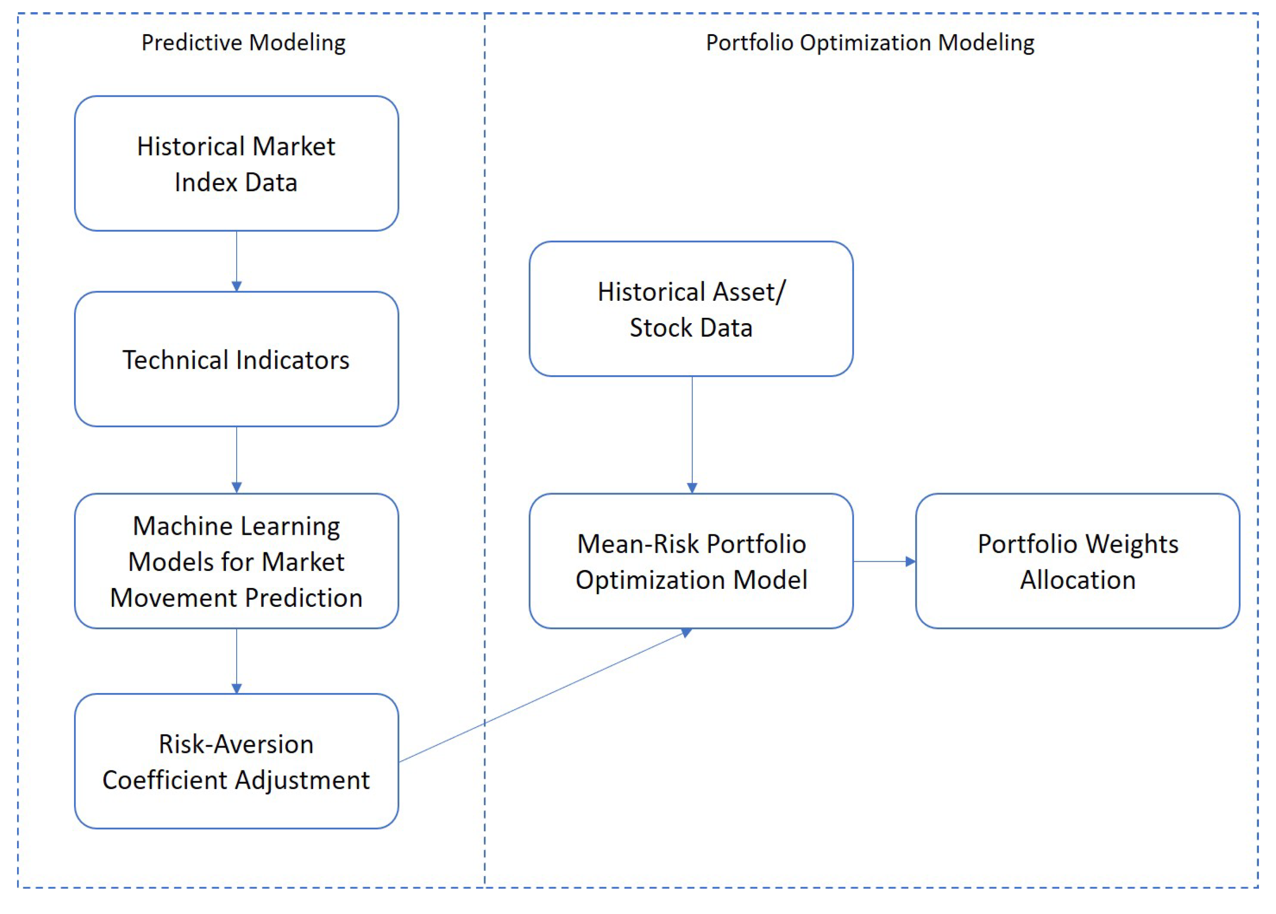
• A specific market is selected (e.g., S&P 500), historical information of the market index and a set of assets that belong to that market are collected. A window of $\tau$ periods are used as in-sample periods to build the machine learning models in a cross-validation manner and to construct the NMG portfolios. In our tests, $\tau$ is selected to be 260 that covers weekly returns over 5 years.
• Within the in-sample periods up to time period t, the 14 technical indicators (i.e., SMA, WMA, EMA, MACD, RSI, ADX, CCI, SMI, EMV, MFI, CMF, VWAP, BBands and SAR) are computed from the index value and are fed to the two machine learning models (i.e., LR, XGBoost) to obtain the market movement with predicted probabilities ${\lambda }_{t+1}$. The tuning parameters of machine learning models are selected via cross-validation. Using the new or updated risk-aversion coefficient, we solve the NMG model to obtain portfolio weights within the training window.
• We carry out the rolling horizon procedure each time by adding the data of the next week (period) in the out-of-sample periods and dropping the data of the earliest week from the in-sample periods. The technical indicators, machine learning models results, and portfolio optimization models are updated on a weekly basis.
• We repeat this procedure until the end of the selected dataset, which generates $T-\tau$ portfolios. The weight of asset i in time period t is denoted by $w_{it}$, for $t=\tau ,\dots ,T-1$. Holding the portfolio weights $w_{it}$ for one week gives the out-of-sample return at time $t+1:R_{t+1}={\sum }_{i=1}^I{w}_{it}{r}_{i,t+1}$, where $r_{i,t+1}$ denotes the return of asset i in out-of-sample period $t+1$. We then evaluate the out-of-sample portfolio performance and compare them to other benchmarks.

We emphasize that our proposed framework is a general framework that can be easily extended to employ various types of technical indicators, machine learning classification models with predicted probabilities, and mean-risk portfolio optimization models, not limited to the ones presented in the current paper. We refer interested readers to Colby (2002); Cervelló-Royo and Guijarro (2020) and Fabozzi et al. (2010) for more choices of technical indicators, machine learning algorithms, and mean-risk portfolio models.

4. Computational Tests

In this section, we carry out a series of tests with empirical data to evaluate the portfolio performance generated by the machine learning integrated Mean-Gini portfolio rebalance framework. Section 4.1 introduces the data sets and experimental design. Section 4.2 describes the metrics to evaluate portfolio performances. Section 4.3 provides the results of machine learning models and derives insights regarding the out-of-sample performance of the risk-aversion adjusted portfolios.

4.1. Data and Experimental Design

Our experiments were conducted with data from Standard & Poor’s 500 (S&P500) stock market, which is a stock market index based on the capitalization of the 500 representative US companies. The entire dataset were downloaded via R programming language using the getSymbols function within the quantmod package. We collected the data of S&P 500 index, 25 risky assets, and 1 risk-free asset (13 Week Treasury Bill) from 01/09/1995 to 12/31/2018 with 1252 weekly returns. These 26 assets constitute the asset candidates pool to construct the portfolios. The tickers and companies of the 26 assets are listed in

Table 2. List of Assets.

S&P 500 Sectors	Ticker	Company Name
Communication Services	DIS	The Walt Disney Company
	VZ	Verizon Communications Inc.
Consumer Discretionary	HD	The Home Depot, Inc.
	MCD	McDonald’s Corporation
	NKE	NIKE, Inc.
Consumer Staples	KO	The Coca-Cola Company
	PG	The Procter Gamble Company
	SYY	Sysco Corporation
	WMT	Walmart Inc.
Energy	CVX	Chevron Corporation
	XOM	Exxon Mobil Corporation
Financials	AXP	American Express Company
	JPM	JPMorgan Chase Co.
Health Care	JNJ	Johnson Johnson
	MRK	Merck Co., Inc.
	PFE	Pfizer Inc.
	WBA	Walgreens Boots Alliance, Inc.
Industrials	BA	The Boeing Company
	CAT	Caterpillar Inc.
	MMM	3M Company
	UTX	Raytheon Technologies Corporation
Information Technology	AAPL	Apple Inc.
	CSCO	Cisco Systems, Inc.
	IBM	International Business Machines Corporation
	INTC	Intel Corporation
-	IRX	13-Week Treasury Bill

. The adjusted close prices were used to compute the technical indicators. We selected the 25 risky assets in Table 2 with three factors—(i) The selected assets have no missing values within the studied time horizon; (ii) The selected assets are not high volatile assets, with volatility lower than 0.5; (iii) The selected assets are diversified to reflect the market index. The selected 25 assets cover 9 out of 11 S&P 500 sectors. The selected 25 assets remained in the S&P 500 index during the testing period. This could potentially lead to a survivor bias and a possible slightly skewed over-performance of the portfolios when compared to the S&P index. However, we note that the comparisons among the constructed portfolios are valid considering they use the same dataset. In addition, similar empirical evaluations of the asset universe have been commonly employed in the literature (see, e.g., Disatnik and Benninga 2007 and Urbán and Ormos 2012).

We conducted the tests following the rolling-horizon approach with a training window for 260 periods (5 years). In each window, we built the logistic regression and XGBoost models, and predicted the probability of the market going up in the 261st period. The predicted probability will be used as the risk-aversion coefficient $\lambda$ in the NMG model to construct the Mean-Gini portfolio. We carried the portfolio weights into the 261st period and obtained a portfolio return and validated the prediction accuracy of the machine learning models. We then dropped the data of the 1st week and added the data of the 261st week to build the second training window and repeated the training of the machine learning models and constructing Mean-Gini portfolios. We repeated this procedure until the end of the entire dataset.

For comparison purposes, besides the two Mean-Gini portfolios constructed via logistic regression and XGBoost with risk-aversion adjustment, we used the following four benchmarks: (1) Mean-Gini portfolio with fixed risk-aversion coefficient $\lambda =0.5$; (2) The equal weights portfolio, that is, the capital is equally assigned into the 26 assets over all testing periods; (3) The S&P 500 market index; (4) The classical minimal variance (MinVar) portfolio (i.e., a portfolio that minimizes the variance of returns). We note that there are many candidates on the mean-variance efficient frontier to be selected, we pick this MinVar as a baseline for comparison.

The R software was used to compute the technical indicators from the S&P 500 index and build the machine learning models via a cross-validation procedure to generate the market movement predictions. The AMPL modeling language was used to formulate the NMG and MinVar portfolio optimization problem, and each problem instance was solved by the commercial solver Cplex with version 12.6. All tests were conducted on a 64-bit desktop with Intel(R) Core(TM) i5-6500 processor, running at 3.2GHz CPU and with 8GB RAM.

4.2. Performance Metrics

To evaluate the out-of-sample performance of the portfolios, we employed the following six metrics based on time-series returns and asset weights.

• The out-of-sample average weekly return:

  $$R_a=\frac{1}{T-\tau }\sum _{t=\tau }^{T-1}\sum _{i=1}^I{w}_{it}{r}_{i,t+1}.$$

  (18)
• The out-of-sample standard deviation:

  $$\sigma =\sqrt{\frac{1}{T-\tau -1}\sum _{t=\tau }^{T-1}{(R_{t+1}-R_a)}^2}.$$

  (19)
• The out-of-sample Gini’s Mean Difference (GMD):

  $$G_{out}=\frac{1}{(T-\tau -1)(T-\tau )}\sum _{t=\tau }^{T-1}\sum _{t^{\prime }>t}^T|R_t^j-R_{t^{\prime }}^j|.$$

  (20)
• The out-of-sample Sharpe ratio:

  $$SR=\frac{R_a}{\sigma }=\frac{R_a}{\sqrt{\frac{1}{T-\tau -1}{\displaystyle \sum _{t=\tau }^{T-1}}{(R_{t+1}-R_a)}^2}}.$$

  (21)
• The out-of-sample cumulative return:

  $$R_c=\prod _{t=\tau }^{T-1}(1+R_{t+1})-1.$$

  (22)
• The out-of-sample annualized return:

  $$R_{anu}={(R_c+1)}^{\frac{1}{(T-\tau -1)/52}}-1.$$

  (23)

4.3. Computational Results and Insights

In this section, we first present the results of logistic regression and XGBoost models for market trend predictions, then assess the out-of-sample performance of the constructed portfolios.

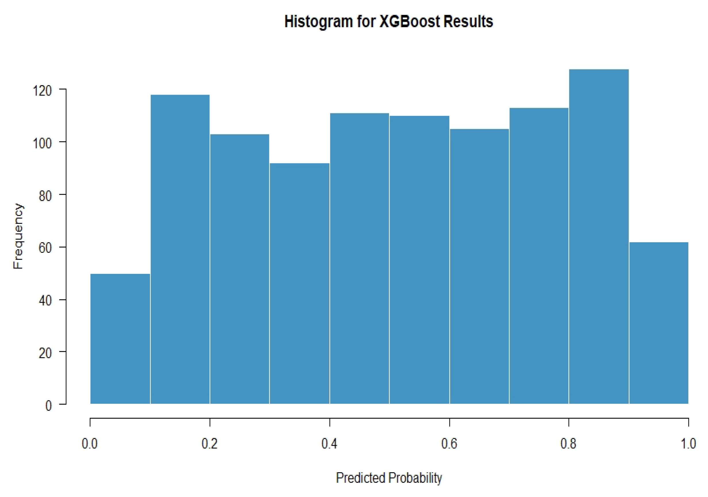
4.3.1. Results of Machine Learning Models

We compared the prediction accuracy of the two models by setting a cutoff value for probability level $p=0.5$, that is, if the predicted probability is greater than or equal to 0.5, then the market is predicted to move upward; otherwise, it is predicted to move downward. The prediction accuracy of logistic regression model is 0.5857. The accuracy of XGBoost is 0.5958, which is 1.01% better than logistic regression.

We generated a total of 37 predictors with different parameter settings of the 14 employed technical indicators (see Table 1 for more details). Figure 2 displays the relative importance of different predictors with the XGBoost algorithm averaged over all 992 windows. The five most important technical indicators are EMV, MACD, RSI, ADX and SMI. The performance of the technical indicators is sensitive to the parameters defining them, among which the number of periods to average over plays a critical role. EMV$(n=10)$ taking the average over 10 periods is the most important predictor. Considering that the other two versions of EMV with $n=3$ and $n=5$ do not appear in the top list, using a longer average period for EMV is more appropriate to train the model. A similar pattern can be detected for the RSI indicator. All three versions of RSI with $n=10,5,3$ are important predictors, while RSI$(n=10)$ is more important than RSI$(n=5)$, then followed by RSI$n=3$. The impacts of periods on MACD and ADX are the opposite, that is, the indicators with shorter periods are more important than those with longer periods. For example, MACD$(2,3,3)$ weighs more importantly than MACD$(3,4,5)$, while RSI$(n=10)$ weighs more than RSI$(n=5)$ and RSI$(n=3)$. SMI shows a different pattern that SMI$(n=3)$ has almost identical importance to SMI$(n=10)$, while they are both much better than SMI$(n=5)$.

Figure 3 plots the histogram of the predicted probabilities of the 992 XGBoost models on a 0.1 bin width. The extreme probability predictions, such as $p\in [0,0.1]$ and $p\in [0.9,1.0]$, are relatively small with frequency of 50 and 58, respectively. The highest frequency is found in the interval of $[0.8,0.9]$ with 122. A bi-modal distribution pattern can be roughly observed with a symmetric line at $p=0.5$.

4.3.2. Evaluation of Portfolio Out-of-Sample Performance

We next present the results of the out-of-sample portfolio performance. We compared the performance of six portfolios as follows: (1) LR: the NMG portfolios generated with risk-aversion adjustment by logistic regression model; (2) XGBoost: the NMG portfolios generated with risk-aversion adjustment by XGBoost model; (3) $\lambda =0.5$: the NMG portfolios with fixed risk-aversion coefficient being equal to 0.5; (4) Equal Weights: the portfolio with equal weights assigned across all assets; (5) S&P 500: the S&P 500 market index; (6) MinVar: the portfolio with minimal variance.

Table 3. Out-of-Sample Performance Comparisons.

	LR	XGBoost	$\mathit{\lambda }=0.5$	Equal Weights	S&P 500	MinVar
Average Return	0.33%	0.35%	0.24%	0.22%	0.08%	0.03%
Standard Deviation	3.42%	3.68%	2.76%	2.29%	2.42%	0.04%
GMD	1.77%	1.83%	1.48%	1.20%	1.26%	0.02%
Sharpe Ratio	0.0970	0.0948	0.0878	0.0955	0.0335	0.8820
Cumulative Return	1390.65%	1511.73%	655.62%	574.16%	66.61%	36.07%
Annualized Return	15.28%	15.76%	11.23%	10.57%	2.72%	1.63%

displays the performance comparisons of the above six portfolios with respect to the performance metrics including the out-of-sample average return, standard deviation, Gini’s Mean Difference, Sharpe ratio, cumulative return, annualized return. Figure 4 shows the time-series cumulative returns of the six portfolios across the out-of-sample periods.

The performance of portfolios (LR and XGBoost) generated by our proposed machine learning integrated portfolio rebalance framework shows superior performance compared to the other four benchmark portfolios in terms of return measures, that is, average return, cumulative return, and annualized return. Suppose the investor is profit-driven, then the LR and XGBoost portfolios are convincing choices to be adopted. The XGBoost portfolios display the best performance among all portfolios with respect to average return (0.35%), cumulative return (1511.73%) and annualized return (15.76%). The LR portfolios have a close performance to the XGBoost portfolios, with an average return of 0.33%, cumulative return of 1390.65% and an annualized return of 15.28%. In terms of cumulative return at the end of the testing periods, XGBoost (resp. LR) portfolios is 1.31, 1.63, 21.70 and 40.91 (resp. 1.12, 1.42, 19.88 and 37.55) times better than $\lambda =0.5$, Equal Weights, S&P 500 index, and MinVar portfolio, respectively.

The MinVar portfolio has the best performance with respect to the out-of-sample risk measures such as standard deviation and Gini’s Mean Difference. The MinVar portfolio is the most conservative and diversified portfolio. MinVar portfolio puts weights into all 26 assets across all 992 periods, while focusing more on risk-free assets. Each constructed MinVar portfolio invests more than 90% of the capital into the risk-free asset, leading to very low values of risk measures (e.g., standard deviation at 0.04% and GMD at 0.02%), as well as low return measures (e.g., average return at 0.03%, cumulative return at 36.07% and annualized return 1.63%). The lowest standard deviation of MinVar leads to its highest Sharpe ratio at 0.8820, which dominates all 5 other portfolios. Excluding the MinVar portfolio, the LR portfolio has the highest Sharpe ratio. The XGBoost portfolio does not beat the Equal Weights portfolios with respect to Sharpe ratio (0.0948 vs. 0.0955), but it still beats the $\lambda =0.5$ portfolio (0.0878) and S&P 500 (0.0335). The performance of the portfolios is consistent in terms of standard deviation and GMD, the MinVar has the lowest value, followed by Equal Weights, S&P 500, $\lambda =0.5$, then by LR and XGBoost.

From Figure 4, the LR and XGBoost portfolios show dominance over the benchmarks S&P 500 and MinVar portfolio across the testing periods. The dominance relationship becomes more significant starting in 2009, after the financial crisis in 2008. The portfolios generated by our machine learning integrated framework with risk-aversion adjustment provide convincing results, by outperforming the one without risk-aversion adjustment ($\lambda =0.5$), and the other three classical benchmarks (Equal Weights, S&P 500 and MinVar) in terms of average return, cumulative return and annualized return, which also display great performance with respect to Sharpe ratio.

5. Summary and Future Studies

In this paper, we propose a machine learning integrated mean-risk portfolio rebalance framework with risk-aversion adjustment in a multi-period setting. When rebalancing the portfolio, a set of technical indicators are fed to the machine learning classification models to predict the probability of market movement, and investors can thus adjust the risk-aversion coefficient accordingly in the mean-risk optimization to obtain portfolio weights. In our study, we employ the Gini’s Mean Difference as the risk measure in our portfolio optimization model. We use 14 popular technical indicators generated from a market index (S&P 500) to train the machine learning models (logistic regression and XGBoost). Within a rolling-horizon procedure, we conduct an extensive set of empirical tests to assess the prediction results of the machine learning models and evaluate the out-of-sample performance of the resulting portfolios. We find that XGBoost model provides better performance prediction. The LR and XGBoost portfolios generated by our proposed framework show great performance in terms of average return, cumulative return and annualized return compared to the three other benchmarks.

For future research, we aim to expand the proposed framework to the index tracking optimization problem (see for example, García et al. 2018a) that utilizes the predictive modeling power to detect the market movement trend for better tracking performance. Moreover, we would also like to incorporate more practical constraints when building the mean-risk portfolio optimization models, such as the bound and cardinality constraints (see Guijarro and Tsinaslanidis 2019), and evaluate the performance of the proposed framework with a larger as well as a more comprehensive dataset.

References

1. Ahmadi-Javid, Amir. 2012. Entropic value-at-risk: A new coherent risk measure. Journal of Optimization Theory and Applications 155: 1105–23. [Google Scholar] [CrossRef]
2. Ahn, Dong-Hyun, Jennifer Conrad, and Robert Dittmar. 2003. Risk adjustment and trading strategies. Review of Financial Studies 16: 459–85. [Google Scholar] [CrossRef]
3. Artzner, Philippe, Freddy Delbaen, Jean-Marc Eber, and David Heath. 1999. Coherent measures of risk. Mathematical Finance 9: 203–28. [Google Scholar] [CrossRef]
4. Basel Committee on Banking Supervision. 2004. International Convergence of Capital Measurement and Capital Standards: A Revised Framework. Basel: BIS. [Google Scholar]
5. Brock, William, Josef Lakonishok, and Blake LeBaron. 1992. Simple technical trading rules and the stochastic properties of stock returns. The Journal of Finance 47: 1731–64. [Google Scholar] [CrossRef]
6. Cervelló-Royo, Roberto, and Francisco Guijarro. 2020. Forecasting stock market trend: A comparison of machine learning algorithms. Finance, Markets and Valuation 6: 37–49. [Google Scholar]
7. Chen, Jiah-Shing, Chia-Lan Chang, Jia-Li Hou, and Yao-Tang Lin. 2008. Dynamic proportion portfolio insurance using genetic programming with principal component analysis. Expert Systems with Applications 35: 273–78. [Google Scholar] [CrossRef]
8. Chen, Tianqi, and Carlos Guestrin. 2016. Xgboost: A scalable tree boosting system. In Proceedings of the 22nd Acm Sigkdd International Conference on Knowledge Discovery and Data Mining. New York: ACM, pp. 785–94. [Google Scholar]
9. Chen, Yan, Shingo Mabu, and Kotaro Hirasawa. 2010. A model of portfolio optimization using time adapting genetic network programming. Computers & Operations Research 37: 1697–707. [Google Scholar]
10. Colby, Robert W. 2002. The Encyclopedia of Technical Market Indicators. New York: McGraw-Hill. [Google Scholar]
11. Conrad, Jennifer, and Gautam Kaul. 1998. An anatomy of trading strategies. Review of Financial Studies 11: 489–519. [Google Scholar] [CrossRef]
12. Covel, Michael. 2004. Trend Following: How Great Traders Make Millions in Up or Down Markets. Upper Saddle River: FT Press. [Google Scholar]
13. Covel, Michael. 2009. Trend Following: Learn to Make Millions in Up Or Down Markets. Upper Saddle River: FT Press. [Google Scholar]
14. DeMiguel, Victor, Lorenzo Garlappi, Francisco Nogales, and Raman Uppal. 2009. A generalized approach to portfolio optimization: Improving performance by constraining portfolio norms. Management Science 55: 798–812. [Google Scholar] [CrossRef] [Green Version]
15. Disatnik, David, and Simon Benninga. 2007. Shrinking the covariance matrix. The Journal of Portfolio Management 33: 55–63. [Google Scholar] [CrossRef]
16. Duffie, Darrell, and Jun Pan. 1997. An overview of value at risk. The Journal of Derivatives 4: 7–49. [Google Scholar] [CrossRef] [Green Version]
17. Fabozzi, Frank, Dashan Huang, and Guofu Zhou. 2010. Robust portfolios: Contributions from operations research and finance. Annals of Operations Research 176: 191–220. [Google Scholar] [CrossRef] [Green Version]
18. Fama, Eugene, and Marshall Blume. 1966. Filter rules and stock-market trading. Journal of Business 39: 226–41. [Google Scholar] [CrossRef]
19. Freitas, Fabio, Alberto De Souza, and Ailson de Almeida. 2009. Prediction-based portfolio optimization model using neural networks. Neurocomputing 72: 2155–70. [Google Scholar] [CrossRef]
20. Gaivoronski, Alexei, and Georg Pflug. 2004. Value-at-Risk in portfolio optimization: Properties and computational approach. The Journal of Risk 7: 1–31. [Google Scholar] [CrossRef] [Green Version]
21. García, Fernando, Francisco Guijarro, and Javier Oliver. 2018a. Index tracking optimization with cardinality constraint: A performance comparison of genetic algorithms and tabu search heuristics. Neural Computing and Applications 30: 2625–41. [Google Scholar] [CrossRef]
22. García, Fernando, Francisco Guijarro, Javier Oliver, and Rima Tamošiūnienė. 2018b. Hybrid fuzzy neural network to predict price direction in the German DAX-30 index. Technological and Economic Development of Economy 24: 2161–78. [Google Scholar] [CrossRef]
23. Geweke, John, and Gianni Amisano. 2010. Comparing and evaluating bayesian predictive distributions of asset returns. International Journal of Forecasting 26: 216–30. [Google Scholar] [CrossRef]
24. Gorgulho, António, Rui Neves, and Nuno Horta. 2011. Applying a GA kernel on optimizing technical analysis rules for stock picking and portfolio composition. Expert systems with Applications 38: 14072–85. [Google Scholar] [CrossRef]
25. Guijarro, Francisco, and Prodromos Tsinaslanidis. 2019. A surrogate similarity measure for the mean-variance frontier optimisation problem under bound and cardinality constraints. Journal of the Operational Research Society, 1–16. [Google Scholar] [CrossRef]
26. Hu, Hongping, Li Tang, Shuhua Zhang, and Haiyan Wang. 2018. Predicting the direction of stock markets using optimized neural networks with google trends. Neurocomputing 285: 188–95. [Google Scholar] [CrossRef]
27. Ji, Ran, Miguel Lejeune, and Srinivas Prasad. 2017a. Dynamic portfolio optimization with risk-aversion adjustment utilizing technical indicators. Paper presented at the 2017 20th International Conference on Information Fusion (Fusion), Xi’an, China, July 10–13; Piscataway: IEEE, pp. 1787–94. [Google Scholar]
28. Ji, Ran, Miguel Lejeune, and Srinivas Prasad. 2017b. Properties, formulations, and algorithms for portfolio optimization using mean-gini criteria. Annals of Operations Research 248: 305–43. [Google Scholar] [CrossRef]
29. Ji, Ran, Miguel Lejeune, and Srinivas Prasad. 2018. Interactive portfolio optimization using Mean-Gini criteria. In Financial Decision Aid Using Multiple Criteria. Berlin and Heidelberg: Springer, pp. 49–91. [Google Scholar]
30. Ji, Ran, K. C. Chang, and Zhenlong Jiang. 2019. Risk-aversion adjusted portfolio optimization with predictive modeling. Paper presented at the 2019 22th International Conference on Information Fusion (FUSION), Ottawa, ON, Canada, July 2–5; Piscataway: IEEE, pp. 1–8. [Google Scholar]
31. Ko, Po-Chang, and Ping-Chen Lin. 2008. Resource allocation neural network in portfolio selection. Expert Systems with Applications 35: 330–37. [Google Scholar] [CrossRef]
32. Konno, Hiroshi, and Hiroaki Yamazaki. 1991. Mean-absolute deviation portfolio optimization model and its applications to Tokyo stock market. Management Science 37: 519–31. [Google Scholar] [CrossRef] [Green Version]
33. Kwon, Ki-Yeol, and Richard Kish. 2002. Technical trading strategies and return predictability: NYSE. Applied Financial Economics 12: 639–53. [Google Scholar] [CrossRef]
34. Lo, Andrew, Harry Mamaysky, and Jiang Wang. 2000. Foundations of technical analysis: Computational algorithms, statistical inference, and empirical implementation. The Journal of Finance 55: 1705–70. [Google Scholar] [CrossRef] [Green Version]
35. Markowitz, Harry. 1952. Portfolio selection. Journal of Finance 7: 77–91. [Google Scholar]
36. Markowitz, Harry. 1959. Portfolio Selection: Efficient Diversification of Investments. New York: Wiley. [Google Scholar]
37. Markowitz, Harry, Peter Todd, Ganlin Xu, and Yuji Yamane. 1993. Computation of mean-semivariance efficient sets by the critical line algorithm. Annals of Operations Research 45: 307–17. [Google Scholar] [CrossRef]
38. Ni, Li-Ping, Zhi-Wei Ni, and Ya-Zhuo Gao. 2011. Stock trend prediction based on fractal feature selection and support vector machine. Expert Systems with Applications 38: 5569–76. [Google Scholar] [CrossRef]
39. Ogryczak, Włodzimierz, and Andrzej Ruszczyński. 1999. From stochastic dominance to mean-risk models: Semi-deviations as risk measures. European Journal of Operational Research 116: 33–50. [Google Scholar] [CrossRef] [Green Version]
40. Ogryczak, Włodzimierz, and Andrzej Ruszczyński. 2001. On consistency of stochastic dominance and mean-semideviations models. Mathematical Programming 89: 217–32. [Google Scholar] [CrossRef]
41. Ringuest, Jeffrey, Samuel Graves, and Randy Case. 2004. Mean-Gini analysis in R&D portfolio selection. European Journal of Operational Research 154: 157–69. [Google Scholar]
42. Rockafellar, Tyrrell, and Stanislav Uryasev. 2000. Optimization of conditional Value-at-Risk. Journal of Risk 2: 21–42. [Google Scholar] [CrossRef] [Green Version]
43. Schwager, Jack. 1993. Market Wizards: Interviews with Top Traders. New York: Collins. [Google Scholar]
44. Schwager, Jack. 1995. The New Market Wizards: Conversations with America’s Top Traders. New York: Wiley. [Google Scholar]
45. Sehgal, Ruchika, and Aparna Mehra. 2017. Worst-case analysis of Gini mean difference safety measure. Journal of Industrial & Management Optimization, 13. [Google Scholar] [CrossRef] [Green Version]
46. Shalit, Haim, and Doron Greenberg. 2013. Hedging with stock index options: A Mean-Extended Gini approach. Journal of Mathematical Finance 3: 119–29. [Google Scholar] [CrossRef] [Green Version]
47. Shalit, Haim, and Shlomo Yitzhaki. 1984. Mean-Gini, portfolio theory, and the pricing of risky assets. The Journal of Finance 39: 1449–68. [Google Scholar] [CrossRef]
48. Thawornwong, Suraphan, and David Enke. 2004. Forecasting stock returns with artificial neural networks. In Neural Networks in Business Forecasting. Hershey: IGI Global, pp. 47–79. [Google Scholar]
49. Urbán, Andrásand Mihály Ormos. 2012. Performance analysis of equally weighted portfolios: USA and Hungary. Acta Polytechnica Hungarica 9: 155–68. [Google Scholar]
50. Yitzhaki, Shlomo. 1982. Stochastic dominance, mean variance and Gini’s mean difference. American Economic Review 72: 178–85. [Google Scholar]
51. Yitzhaki, Shlomo. 1983. On an extension of the Gini inequality index. International Economic Review 24: 617–28. [Google Scholar] [CrossRef]
52. Zhou, Xiaocong, Jouchi Nakajima, and Mike West. 2014. Bayesian forecasting and portfolio decisions using dynamic dependent sparse factor models. International Journal of Forecasting 30: 963–80. [Google Scholar] [CrossRef]
53. Zhu, Shushang, Duan Li, and Shouyang Wang. 2009. Robust portfolio selection under downside risk measures. Quantitative Finance 9: 869–85. [Google Scholar] [CrossRef]
Figure 1. Overview of Machine Learning Integrated Portfolio Rebalance Framework.
Jrfm 13 00155 g001
Figure 2. Importance Plot of XGBoost Model.
Jrfm 13 00155 g002
Figure 3. Distribution of Predicted Probabilities of XGBoost Model.
Jrfm 13 00155 g003
Figure 4. Time-Series Cumulative Returns Comparisons.
Jrfm 13 00155 g004