Robust Inference in the Capital Asset Pricing Model Using the Multivariate t-distribution

Abstract

In this paper, we consider asset pricing models under the multivariate t-distribution with finite second moment. Such a distribution, which contains the normal distribution, offers a more flexible framework for modeling asset returns. The main objective of this work is to develop statistical inference tools, such as parameter estimation and linear hypothesis tests in asset pricing models, with an emphasis on the Capital Asset Pricing Model (CAPM). An extension of the CAPM, the Multifactor Asset Pricing Model (MAPM), is also discussed. A simple algorithm to estimate the model parameters, including the kurtosis parameter, is implemented. Analytical expressions for the Score function and Fisher information matrix are provided. For linear hypothesis tests, the four most widely used tests (likelihood-ratio, Wald, score, and gradient statistics) are considered. In order to test the mean-variance efficiency, explicit expressions for these four statistical tests are also presented. The results are illustrated using two real data sets: the Chilean Stock Market data set and another from the New York Stock Exchange. The asset pricing model under the multivariate t-distribution presents a good fit, clearly better than the asset pricing model under the assumption of normality, in both data sets.

1. Introduction

The Capital Asset Pricing Model (CAPM) is one of the most important asset pricing models in financial economics. It is widely used in estimating the cost of capital for companies and measuring portfolio (or investment fund) performance, among others applications; see, for instance, Campbell et al. (1997), Amenc and Le Sourd (2003), Broquet et al. (2004), Levy (2012) and Ejara et al. (2019).

The CAPM framework provides financial practitioners with a measure of $beta$ (or systematic risk) for entire stock markets, industry sub-sectors, and individual equities (Pereiro 2010).

The literature on the CAPM based on the multivariate normal distribution is vast, as seen, for instance, in the works published by Elton and Gruber (1995), Campbell et al. (1997), Broquet et al. (2004), Francis and Kim (2013), Johnson (2014), Brandimarte (2018) and Mazzoni (2018). However, multivariate normality is not required to ensure the validity of the CAPM. In fact, it is well known that the CAPM is still valid within the class of elliptical distributions, of which multivariate normal and multivariate t-distributions are special cases (see Chamberlain 1983; Hamada and Valdez 2008; Ingersoll 1987; Owen and Rabinovitch 1983). It is also well known that in practice, excess returns are not normally distributed. Most financial assets exhibit excess kurtosis, that is to say, returns having distributions whose tails are heavier than those of the normal distribution and present some degree of skewness; see Fama (1965), Blattberg and Gonedes (1974), Zhou (1993), Campbell et al. (1997), Bekaert and Wu (2000), Chen et al. (2001), Hodgson et al. (2002) and Vorknik (2003). Recently Bao et al. (2018) discuss estimation in the univariate CAPM with asymmetric power distributed errors. In this paper, the multivariate version of the CAPM is considered, primarily focusing on modeling non-normal returns due to excess kurtosis.

Within the class of elliptical distributions, the multivariate t-distribution has been widely used to model data with heavy tails. For instance, Lange et al. (1989) discuss the use of the t-distribution in regression and in problems related to multivariate analysis. Sutradhar (1993) has considered a score test aimed at testing if the covariance matrix is equal to some specified covariance matrix using the t-distribution; Bolfarine and Galea (1996) used the t-distribution in structural comparative calibration models, while Pinheiro et al. (2001) used the multivariate t-distribution for robust estimation in linear mixed-effects models. Cademartori et al. (2003), Fiorentini et al. (2003), Galea et al. (2008), Galea et al. (2010) and Kan and Zhou (2017) provide empirical evidence of the usefulness of t-distribution to model stock returns. In addition, statistical inference based on the t-distribution is simple to implement, and the computational cost is considerably low.

Following Kan and Zhou (2017), there are three main reasons for using the t-distribution in modeling returns of financial instruments. (i) empirical evidence shows that this distribution is appropriate for modeling non-normal returns in many situations, (ii) with the algorithms implemented in this paper, the t-distribution has become almost as tractable as the normal one, and (iii) the CAPM is still valid under t-distribution. It is clear that the t-distribution does not describe all the features of the return data. For instance, the volatility variation over time is one of them, for which the GARCH models are very useful. However, according to our experience (see Cademartori et al. 2003; Galea et al. 2008, 2010; Galea and Giménez 2019), and as mentioned by Kan and Zhou (2017), there is little evidence of GARCH effects on the monthly data that are typically used for asset pricing and corporate studies. In addition, when we have a moderate number of assets, for example more than 10, the fit of the GARCH models requires an important computational effort, which limits its application to real data sets. For more details see Harvey and Zhou (1993) and Kan and Zhou (2017).

Thus, the main goal of this paper is to develop statistical inference tools, such as parameter estimation and hypothesis tests, in asset pricing models, with an emphasis on the CAPM, using the multivariate t-distribution. An extension of the CAPM, the multifactor asset pricing model (MAPM), is also discussed. The t-distribution incorporates an additional parameter, which allows modeling returns with high kurtosis. We consider a reparameterization of the multivariate t-distribution with a finite second moment. This enables a more direct comparison with the normal distribution (see Bolfarine and Galea 1996; Sutradhar 1993). Based on Fiorentini et al. (2003), who use the reparameterization of degrees of freedom suggested by Lange et al. (1989) to model financial data, this version of the multivariate t-distribution is adopted to test hypotheses of interest, such as the hypothesis of mean-variance efficiency. The three most widely used tests based on the likelihood function are considered; Wald tests, likelihood-ratio tests, and score tests (also known as Lagrange multiplier tests). Under the assumption of normality, these tests have been discussed in the literature, see for instance Campbell et al. (1997) and Chou and Lin (2002). Recently Kan and Zhou (2017) discuss the likelihood-ratio tests in the CAPM assuming that the excess returns follow a multivariate t-distribution. In this paper, the modeling of the asset returns conditional on market portfolios and the three most widely used tests are considered. Additionally, a fourth test statistic is considered, based on the likelihood proposed by Terrell (2002), the gradient test. To our knowledge this test has not been applied to test hypothesis in asset pricing models.

The article is developed as follows. In Section 2, the CAPM under the multivariate t-distribution, estimation of parameter and tests of mean-variance efficiency are briefly reviewed, and the Generalized Method of Moments is summarized for comparative purposes. In Section 3, the methodology developed in this paper is applied to two real data sets: the Chilean Stock Market data set and another from the New York Stock Exchange, USA. In Section 4, multifactor asset pricing models under the t-distribution are discussed. In Section 5, a conclusion and final comments are included. The appendices contain technical details.

2. Methodology

2.1. The CAPM under the t-Distribution

First, a set of $p\ge 1$ assets of interest is considered, and let $R_i$ denote the return for asset i, with $i=1,\dots ,p$. CAPM specifies that the stock’s expected return is equal to the risk-free rate return plus a risk premium; i.e.,

$$E\left(R_i\right)=R_f+{\beta }_i\{E\left(R_m\right)-R_f\},i=1,\dots ,p,$$

(1)

where $R_f$ is the risk-free interest rate, ${\beta }_i$ is the systematic risk of the asset i, and $R_m$ is the market return. This model was independently derived by Sharpe (1964), Lintner (1965) and Mossin (1966). For these p assets, the excess returns can be described using the following multivariate linear regression model; Gibbons et al. (1989), MacKinlay and Richardson (1991) and Campbell et al. (1997),

$${\mathit{y}}_t=\mathit{\alpha }+\mathit{\beta }{x}_t+{\mathit{ϵ}}_t,t=1,\dots ,n,$$

(2)

where ${\mathit{y}}_t={(y_{1t},\cdots ,y_{pt})}^T$ is a $p\times 1$ vector representing excess returns of the set of p assets of interest in period t such that, $y_{it}=R_{it}-R_{ft}$ denotes the excess return of asset i during period t, $\mathit{\alpha }={({\alpha }_1,\dots ,{\alpha }_p)}^T$ is the intercept vector, $\mathit{\beta }={({\beta }_1,\cdots ,{\beta }_p)}^T$ is the slope vector that corresponds to the sensitivity of the portfolio return to changes in this benchmark return; $x_t=R_{mt}-R_{ft}$ represents the excess return of the market portfolio during period t and finally ${\mathit{ϵ}}_t$ is the errors vector during period t, with mean zero and variance-covariance matrix $\mathsf{\Sigma }$, independent of t, for $t=1,\dots ,n$. If the CAPM holds for this set of assets and the benchmark portfolio is mean-variance efficient, the following restriction on the parameters of model (2) should hold $E\left({\mathit{y}}_t\right)=\mathit{\beta }{x}_t$, for $t=1,\dots ,n$. Hence, this restriction implies a testable hypothesis:

$$H_{\alpha }:\mathit{\alpha }=\mathbf{0}.$$

(3)

Much of the theory of the CAPM is based on the assumption that excess returns follow a multivariate normal distribution; see for instance Campbell et al. (1997), Broquet et al. (2004), Johnson (2014), Brandimarte (2018), Mazzoni (2018) and Galea and Giménez (2019). However, it has been shown that although the assumption of normality is sufficient to generate the model (1), it is not necessary. Chamberlain (1983), Owen and Rabinovitch (1983), Ingersoll (1987), Berk (1997) and most recently Hamada and Valdez (2008) show that (1) can be obtained under the assumption of elliptically symmetric return distributions. In particular, Berk (1997) showed that when agents maximize the expected utility, elliptical symmetry is both necessary and sufficient for the CAPM.

In this paper, we are interested in develop statistical inference tools, estimation and hypothesis tests in asset pricing models supposing that ${\mathit{ϵ}}_t$, the random errors vector following a multivariate t-distribution, has a mean zero and a covariance matrix $\mathsf{\Sigma }$. In effect, we supposed that the density function of ${\mathit{ϵ}}_t$ is given by

$$f\left(\mathit{ϵ}\right)={\left|\mathsf{\Sigma }\right|}^{-1/2}g\left(\delta \right),\delta \ge 0,$$

(4)

where

$$g\left(\delta \right)=k_p\left(\eta \right){\left(1+c\left(\eta \right)\delta \right)}^{-{\displaystyle \frac{1}{2\eta }}(1+\eta p)},$$

with $\delta ={\mathit{ϵ}}^T{\mathsf{\Sigma }}^{-1}\mathit{ϵ}$, $k_p\left(\eta \right)={(c\left(\eta \right)/\pi )}^{p/2}\{\mathsf{\Gamma }((1+\eta p)/2\eta )/\mathsf{\Gamma }(1/2\eta )\}$ and $c\left(\eta \right)=\eta /(1-2\eta )$, $0<\eta <1/2$. In this case we wrote ${\mathit{ϵ}}_t\sim T_p(0,\mathsf{\Sigma },\eta )$. From properties of the t-distribution (see Appendix A), we have, given $x_t$, that ${\mathit{y}}_t\sim T_p(\mathit{\alpha }+\mathit{\beta }{x}_t,\mathsf{\Sigma },\eta )$ independently, $t=1,\dots ,n$. The t-distribution offers a more flexible framework for modeling asset returns. In this distribution $\eta$ is a shape parameter that can be used for adjusting the kurtosis distribution and for providing more robust procedures than the ones that use the normal distribution, with moderate additional computational effort.

Following Campbell et al. (1997), we consider the joint distribution of the excess returns given the excess return market. Specifically, we assume that the excess returns ${\mathit{y}}_1,\dots ,{\mathit{y}}_n$, given the excess return market, are independent random vectors with a multivariate t-distribution and common covariance matrix. Then, the probability density function of ${\mathit{y}}_t$ takes the form of

$$f\left({\mathit{y}}_t\right|\mathit{\theta })={\left|\mathsf{\Sigma }\right|}^{-1/2}g\left({\delta }_t\right),$$

(5)

where, ${\delta }_t={({\mathit{y}}_t-\mathit{\alpha }-\mathit{\beta }{x}_t)}^T{\mathsf{\Sigma }}^{-1}({\mathit{y}}_t-\mathit{\alpha }-\mathit{\beta }{x}_t)$, for $t=1,\dots ,n$. Therefore, the density for a sample of n periods is given by

$$f\left(\mathit{Y}\right|\mathit{\theta })=\prod _{t=1}^{n}f\left({\mathit{y}}_t\right|\mathit{\theta })=\prod _{t=1}^n{\left|\mathsf{\Sigma }\right|}^{-1/2}g\left({\delta }_t\right),$$

(6)

with $\mathit{Y}=({\mathit{y}}_1,\cdots ,{\mathit{y}}_n)$ and $\mathit{\theta }={({\mathit{\alpha }}^T,{\mathit{\beta }}^T,{\mathit{\sigma }}^T,\eta )}^T$, where $\mathit{\sigma }=\mathrm{vech}\left(\mathsf{\Sigma }\right)$ is the $p(p+1)/2$ vector obtained from $\mathrm{vec}\left(\mathsf{\Sigma }\right)$ by deleting from it all of the elements that are above the diagonal of $\mathsf{\Sigma }$.

2.2. Maximum Likelihood Estimation

The logarithm of the likelihood function for the model (6) is given by

$$\mathcal{L}\left(\mathit{\theta }\right)=\sum _{t=1}^n{\mathcal{L}}_t\left(\mathit{\theta }\right),$$

(7)

where ${\mathcal{L}}_t\left(\mathit{\theta }\right)=-{\displaystyle \frac{1}{2}}log\left|\mathsf{\Sigma }\right|+log\left\{g\left({\delta }_t\right)\right\}=log{k}_p\left(\eta \right)-{\displaystyle \frac{1}{2}}log\left|\mathsf{\Sigma }\right|-{\displaystyle \frac{1}{2\eta }}(1+\eta p)log(1+c\left(\eta \right){\delta }_t)$ is the contribution from the tth return to the likelihood, $t=1,2,\dots ,n$.

From (7), the score function is given by

$$\mathcal{U}\left(\mathit{\theta }\right)=\sum _{t=1}^n{U}_t\left(\mathit{\theta }\right),$$

(8)

where $U_t\left(\mathit{\theta }\right)={(U_{t\alpha }^T,U_{t\beta }^T,U_{t\sigma }^T,U_{t\eta })}^T$ with

$$\begin{array}{ccc}\hfill U_{t\alpha }& =& {\omega }_t{\mathsf{\Sigma }}^{-1}{\mathit{ϵ}}_t,\hfill \\ \hfill U_{t\beta }& =& x_t{U}_{t\alpha },\hfill \\ \hfill U_{t\sigma }& =& -\frac{1}{2}{\mathit{D}}_p^T\mathrm{vec}\left({\mathsf{\Sigma }}^{-1}-{\omega }_t{\mathsf{\Sigma }}^{-1}{\mathit{ϵ}}_t{\mathit{ϵ}}_t^T{\mathsf{\Sigma }}^{-1}\right),\mathrm{and}\hfill \\ \hfill U_{t\eta }& =& \frac{1}{2{\eta }^2}\{c\left(\eta \right)p-\beta \left(\eta \right)-{\omega }_{t}c\left(\eta \right){\delta }_t+log(1+c\left(\eta \right){\delta }_t)\},\hfill \end{array}$$

where ${\omega }_t=\left({\displaystyle \frac{1+\eta p}{\eta }}\right)\left({\displaystyle \frac{c\left(\eta \right)}{1+c\left(\eta \right){\delta }_t}}\right)$, for $t=1,\dots ,n$; $\beta \left(\eta \right)=\psi \left({\displaystyle \frac{1}{2\eta }}(1+\eta p)\right)-\psi \left({\displaystyle \frac{1}{2\eta }}\right)$; $\psi \left(x\right)$ is the digamma function and ${\mathit{D}}_p$ is the duplication matrix; see Magnus and Neudecker (2007). It is difficult to obtain the maximum likelihood (ML) estimators from $\mathcal{U}\left(\mathit{\theta }\right)=\mathbf{0}$. The EM algorithm has been suggested frequently to obtain ML estimators in statistical models under the t-distribution, mainly because it leads to a simple implementation of an iteratively weighted estimation procedure. As is well known, the t-distribution is a scale mixture of a normal distribution (see Lange et al. 1989), which facilitates the implementation of the EM algorithm considerably. Then, based on the complete-data log-likelihood function we obtained the expressions of ML estimates (see Liu and Rubin 1995; Shoham 2002; Xie et al. 2007). Thus, in our case, as shown in Appendix B, the ML estimates of $\mathit{\alpha }$, $\mathit{\beta }$, $\mathsf{\Sigma }$ and $\eta$ are obtained as solution of the following equations:

$${\displaystyle \widehat{\mathit{\alpha }}={\overline{\mathit{y}}}_{\omega }-\widehat{\mathit{\beta }}{\overline{x}}_{\omega },\widehat{\mathit{\beta }}=\frac{{\sum }_{t=1}^n{\omega }_t(x_t-{\overline{x}}_{\omega })({\mathit{y}}_t-{\overline{\mathit{y}}}_{\omega })}{{\sum }_{t=1}^n{\omega }_t{(x_t-{\overline{x}}_{\omega })}^2},\widehat{\mathsf{\Sigma }}=\frac{1}{n}\sum _{t=1}^n{\omega }_t{\widehat{\mathit{ϵ}}}_t{\widehat{\mathit{ϵ}}}_t^T,}$$

(9)

and

$${\widehat{\eta }}^{-1}=\frac{2}{a+loga-1}+0.0416\left\{1+erf\left(0.6594log\left(\frac{2.1971}{a+loga-1}\right)\right)\right\},$$

where ${\widehat{\mathit{ϵ}}}_t={\mathit{y}}_t-\widehat{\mathit{\alpha }}-\widehat{\mathit{\beta }}{x}_t$; ${\overline{\mathit{y}}}_{\omega }={\sum }_{t=1}^n{\omega }_t{\mathit{y}}_t/{\sum }_{t=1}^n{\omega }_t$; ${\overline{x}}_{\omega }={\sum }_{t=1}^n{\omega }_t{x}_t/{\sum }_{t=1}^n{\omega }_t$;

$erf\left(x\right)={\displaystyle \frac{2}{\sqrt{\pi }}}{\int }_0^x\exp (-u^2)du$, $a=-(1/n){\sum }_{t=1}^n(v_{t2}-v_{t1})$, with $v_{t1}=(1+p\eta )/(1+c\left(\eta \right){\delta }_t)$ and $v_{t2}=\psi \left({\displaystyle \frac{1+p\eta }{2\eta }}\right)-log\left({\displaystyle \frac{1+c\left(\eta \right){\delta }_t}{2\eta }}\right)$, for $t=1,\dots ,n$. The iterative process given by Equation (9) was implemented in $\mathbf{R}$ language. Note that the normal model ${\omega }_t=1,t=1,\dots ,n$ and the ML estimators of $\mathit{\alpha }$, $\mathit{\beta }$ and $\mathsf{\Sigma }$ correspond to the normal case. Under the $t$-model, the exact marginal distribution of $\widehat{\mathit{\alpha }}$, $\widehat{\mathit{\beta }}$ and $\widehat{\mathsf{\Sigma }}$ are particularly difficult to obtain, but under normal distribution, the estimators of $\mathit{\alpha }$, $\mathit{\beta }$ and $\mathsf{\Sigma }$ have exact marginal distributions (see Campbell et al. 1997).

2.3. Asymptotic Standard Errors

The standard errors of the ML estimators can be estimated using the expected information matrix. For a multivariate elliptically symmetric distribution, Lange et al. (1989) indicated how to compute the expected information matrix. See also Mitchell (1989). In our case, by using score function (8), the Fisher information matrix for $\mathit{\theta }$ in the log-likelihood function defined in (7) assumes the form

$$\mathit{J}=E\left\{\mathcal{U}\left(\mathit{\theta }\right){\mathcal{U}}^T\left(\mathit{\theta }\right)\right\}=\left(\begin{array}{ccc}{\mathit{J}}_{11}& \mathbf{0}& \mathbf{0}\\ \mathbf{0}& {\mathit{J}}_{22}& {\mathit{J}}_{23}\\ \mathbf{0}& {\mathit{J}}_{23}^T& J_{33}\end{array}\right),$$

(10)

where ${\mathit{J}}_{11}$, ${\mathit{J}}_{22}$, ${\mathit{J}}_{23}$ and $J_{33}$ denote information concerning $(\mathit{\alpha },\mathit{\beta })$, $\mathit{\sigma }$, $(\mathit{\sigma },\eta )$ and $\eta$, respectively, and are given by

$$\begin{array}{ccc}\hfill {\mathit{J}}_{11}& =& c_{\alpha }\left(\eta \right)\left(X^{T}X\right)\otimes {\mathsf{\Sigma }}^{-1},\hfill \\ \hfill {\mathit{J}}_{22}& =& \frac{n}{4}{\mathit{D}}_p^T\{2c_{\sigma }\left(\eta \right)({\mathsf{\Sigma }}^{-1}\otimes {\mathsf{\Sigma }}^{-1}){\mathit{N}}_p+(c_{\sigma }\left(\eta \right)-1)(vec{\mathsf{\Sigma }}^{-1}){(vec{\mathsf{\Sigma }}^{-1})}^T\}{\mathit{D}}_p,\hfill \\ \hfill {\mathit{J}}_{23}& =& -\frac{nc\left(\eta \right)c_{\sigma }\left(\eta \right)(p+2)}{{(1+p\eta )}^2}{\mathit{D}}_p^{T}vec{\mathsf{\Sigma }}^{-1},\hfill \\ \hfill J_{33}& =& -\frac{n}{2{\eta }^2}\left\{\left(\frac{p}{{(1-2\eta )}^2}\right)\left(\frac{1+\eta p(1-4\eta )-8{\eta }^2}{(1+\eta p)(1+\eta (p+2\left)\right)}\right)-{\beta }^{\prime }\left(\eta \right)\right\},\hfill \end{array}$$

with ${\mathit{N}}_p=\frac{1}{2}({\mathit{I}}_{p^2}+{\mathit{K}}_p)$ where ${\mathit{K}}_p$ is the commutation matrix of order $p^2\times p^2$ (Magnus and Neudecker 2007); $c_{\alpha }\left(\eta \right)=c_{\sigma }\left(\eta \right)/(1-2\eta )$, $c_{\sigma }\left(\eta \right)=(1+p\eta )/(1+(p+2)\eta )$; and

$${\beta }^{\prime }\left(\eta \right)=-\frac{1}{2{\eta }^2}\left\{{\psi }^{\prime }\left(\frac{1+p\eta }{2\eta }\right)-{\psi }^{\prime }\left(\frac{1}{2\eta }\right)\right\},$$

where ${\psi }^{\prime }\left(z\right)$ denotes the trigamma function. Note that $c_{\alpha }\left(\eta \right)=c_{\sigma }\left(\eta \right)=1$ when $\eta =0$ and ${\mathit{N}}_p{\mathit{D}}_p={\mathit{D}}_p$ (see for instance Magnus and Neudecker 2007), we have to recover the expressions corresponding to the normal case. Here, X is an $n\times 2$ matrix such $X^T=\left(\begin{array}{ccccc}1& ·& ·& ·& 1\\ x_1& ·& ·& ·& x_n\end{array}\right)$ and ⊗ denotes the Kronecker product. The asymptotic sampling distribution of the ML estimator $\widehat{\mathit{\theta }}$ is given by

$$\begin{array}{c}\hfill \sqrt{n}(\widehat{\mathit{\theta }}-\mathit{\theta })\stackrel{\mathcal{D}}{\mapsto }{\mathcal{N}}_r(0,{\mathit{V}}^{-1}),\end{array}$$

where $\mathit{V}={lim}_{n\to \infty }(1/n)\mathit{J}$ and $r=\left\{p\right(p+5)+2\}/2$ is the dimension of $\mathit{\theta }$. To estimate V, we use $\widehat{\mathit{V}}=\mathit{J}\left(\widehat{\mathit{\theta }}\right)/n$.

2.4. Test of Mean-Variance Efficiency

To test $H_{\alpha }:\mathit{\alpha }=\mathbf{0}$ the three classic tests based on the likelihood function are considered, including the Wald test, likelihood-ratio test, and score test; see for instance Boos and Stefanski (2013). Let $\mathit{\theta }={({\mathit{\alpha }}^T,{\mathit{\theta }}_2^T)}^T$, with ${\mathit{\theta }}_2={({\mathit{\beta }}^T,{\mathit{\sigma }}^T,\eta )}^T$ and $\mathcal{U}\left(\mathit{\theta }\right)={(U_{\alpha }^T\left(\mathit{\theta }\right),U_2^T\left(\mathit{\theta }\right))}^T$ the score function (8) partitioned following the partition of $\mathit{\theta }$. In this case, after some algebraic manipulations, the test statistics are given by

$$\begin{array}{cc}\hfill Lr& =nlog\left\{\right|\tilde{\mathsf{\Sigma }}|/|\widehat{\mathsf{\Sigma }}\left|\right\}+2\sum _{t=1}^{n}log\{g\left({\widehat{\delta }}_t\right)/g\left({\tilde{\delta }}_t\right)\},\hfill \\ \hfill Wa& =n{c}_{\alpha }\left(\widehat{\eta }\right){(1+{\overline{x}}^2/s^2)}^{-1}{\widehat{\mathit{\alpha }}}^T{\widehat{\mathsf{\Sigma }}}^{-1}\widehat{\mathit{\alpha }},\hfill \\ \hfill Sc& ={\displaystyle \frac{1}{n{c}_{\alpha }^{-1}\left(\tilde{\eta }\right)}}(1+{\overline{x}}^2/s^2){\mathit{d}}^T{\tilde{\mathsf{\Sigma }}}^{-1}\mathit{d},\hfill \end{array}$$

where $\overline{x}=(1/n){\sum }_{t=1}^n{x}_t$, $s^2=(1/n){\sum }_{t=1}^n{(x_t-\overline{x})}^2$, ${\widehat{\delta }}_t={\widehat{\mathit{ϵ}}}_t^T{\widehat{\mathsf{\Sigma }}}^{-1}{\widehat{\mathit{ϵ}}}_t$, ${\tilde{\delta }}_t={({\mathit{y}}_t-\tilde{\mathit{\beta }}{x}_t)}^T{\tilde{\mathsf{\Sigma }}}^{-1}({\mathit{y}}_t-\tilde{\mathit{\beta }}{x}_t)$; $\widehat{\mathit{\alpha }}$, $\widehat{\mathit{\beta }}$, $\widehat{\mathsf{\Sigma }}$ and $\widehat{\eta }$ are the ML estimators in the model (6); $\tilde{\mathit{\beta }}$, $\tilde{\mathsf{\Sigma }}$ and $\tilde{\eta }$ are the ML estimators of $\mathit{\beta }$, $\mathsf{\Sigma }$ and $\eta$ under $H_{\alpha }$, $\mathit{d}={\sum }_{t=1}^n{\tilde{\omega }}_t({\mathit{y}}_t-\tilde{\mathit{\beta }}{x}_t)$, $\tilde{\mathit{\theta }}$ and $\widehat{\mathit{\theta }}$ are the restricted and unrestricted ML estimators of $\mathit{\theta }$, respectively. Under $H_{\alpha }$, the asymptotic distribution of each of these test statistics is ${\chi }^2\left(p\right)$. Note that $c_{\alpha }\left(\eta \right)=1$ when $\eta =0$ and $Wa=n{(1+{\overline{x}}^2/s^2)}^{-1}{\widehat{\mathit{\alpha }}}^T{\widehat{\mathsf{\Sigma }}}^{-1}\widehat{\mathit{\alpha }}$, which corresponds to the Wald test under normality; see, for instance, Campbell et al. (1997). In addition, under the assumption of multivariate normality, the likelihood-ratio test is given by $Lr=nlog(1+Wa/n)$, and the score test takes the form $Sc=Wa/(1+Wa/n)$. The gradient test Terrell (2002) is also discussed, defined as

$$Ga={\mathcal{U}}^T\left(\tilde{\mathit{\theta }}\right)(\widehat{\mathit{\theta }}-\tilde{\mathit{\theta }}).$$

(11)

Since $U_2\left(\tilde{\mathit{\theta }}\right)=\mathbf{0}$, the gradient statistic in (11) can be written as $Ga=U_{\alpha }^T\left(\tilde{\mathit{\theta }}\right)\widehat{\mathit{\alpha }}={\mathit{d}}^T{\tilde{\mathsf{\Sigma }}}^{-1}\widehat{\mathit{\alpha }}$. Note that $Ga$ is attractive, as it is simple to compute and does not involve knowledge of the Fisher information matrix (10), unlike $Wa$ and $Sc$. Asymptotically, $Ga$ has a chi-square distribution with p degrees of freedom under $H_{\alpha }$. For more details and applications of this test, see Terrell (2002) and Lemonte (2016). However, in this case, under the normality assumption, the gradient statistic does not offer an alternative to test the hypothesis of mean-variance efficiency since $Sc=Ga$, see Appendix D.

To calculate the values of the statistics $Lr,Sc$ and $Ga$, it is necessary to estimate $\mathit{\theta }$ under $H_{\alpha }$. The EM algorithm leads to the following equations to obtain the ML estimates of $\mathit{\beta }$, $\mathsf{\Sigma }$ and $\eta$ under $H_{\alpha }$:

$${\displaystyle \tilde{\mathit{\beta }}=\frac{{\sum }_{t=1}^n{\omega }_t{x}_t{\mathit{y}}_t}{{\sum }_{t=1}^n{\omega }_t{x}_t^2},\tilde{\mathsf{\Sigma }}=\frac{1}{n}\sum _{t=1}^n{\omega }_t({\mathit{y}}_t-\tilde{\mathit{\beta }}{x}_t){({\mathit{y}}_t-\tilde{\mathit{\beta }}{x}_t)}^T}$$

and

$${\tilde{\eta }}^{-1}=\frac{2}{a+loga-1}+0.0416\left\{1+erf\left(0.6594log\left(\frac{2.1971}{a+loga-1}\right)\right)\right\},$$

where $a=-(1/n){\sum }_{t=1}^n(v_{t2}-v_{t1})$, with $v_{t1}=(1+p\eta )/(1+c\left(\eta \right){\tilde{\delta }}_t)$ and $v_{t2}=\psi \left({\displaystyle \frac{1+p\eta }{2\eta }}\right)-log\left({\displaystyle \frac{1+c\left(\eta \right){\tilde{\delta }}_t}{2\eta }}\right)$, for $t=1,\dots ,n$.

2.5. Model Assessment and Outlier Detection

Any statistical analysis should include a critical analysis of the model assumptions. Following Lange et al. (1989), in this work the Mahalanobis distance is used to assess the fit of the CAPM. In effect, the random variables

$$F_t=\left({\displaystyle \frac{1}{1-2\eta }}\right){\displaystyle \frac{{\delta }_t}{p}}\sim F(p,1/\eta )$$

for $t=1,\dots ,n$. Substituting the ML estimators yields ${\widehat{F}}_t=F_t\left(\widehat{\mathit{\theta }}\right)$, which has asymptotically the same F distribution as $F_t$, $t=1,\dots ,n$. Using the Wilson-Hilferty approximation,

$$z_t=\frac{\left(1-{\displaystyle \frac{2\eta }{9}}\right){\widehat{F}}_t^{1/3}-\left(1-{\displaystyle \frac{2}{9p}}\right)}{\sqrt{{\displaystyle \frac{2\eta }{9}}{\widehat{F}}_t^{2/3}+{\displaystyle \frac{2}{9p}}}}$$

(12)

for $t=1,\dots ,n$, with an approximately standard normal distribution. Thus, a $QQ$-plot of the transformed distances $\{z_1,\dots ,z_n\}$ can be used to evaluate the fit of the CAPM under the multivariate t-distribution. For $\eta =0$, the transformed distances are simplified to $z_t=\{{\widehat{F}}_t^{1/3}-(1-2/9p)\}/\sqrt{2/9p}$ and can be used to assess of fit of the CAPM under the assumption of normality. Additionally, the Mahalanobis distance can be used for multivariate outlier detection. In effect, larger than expected values of the Mahalanobis distance, ${\widehat{F}}_t$, $t=1,\dots ,n$, identify outlying cases (see Lange et al. 1989).

2.6. Generalized Method of Moments Tests

If the iid multivariate t assumption of random errors is violated, hypothesis (3) can be tested using the Generalized Method of Moments (GMM) (see Hansen 1982). No distributional assumptions are needed other than the data being stationary and ergodic. With the GMM framework, the random errors can be both serially dependent and conditionally heteroskedastic. From (2), we have ${\mathit{ϵ}}_t={\mathit{y}}_t-\mathit{\alpha }-\mathit{\beta }{x}_t$, for $t=1,\dots ,n$. The idea of the GMM approach (see Hansen 1982), is to use sample moments conditions to replace the population moment conditions of the model restrictions. The relevant population moment conditions are $E\left({\mathit{ϵ}}_t\right)=\mathbf{0}$ and $E\left(x_t{\mathit{ϵ}}_t\right)=\mathbf{0}$, for $t=1,\dots ,n$.

Define $2p\times 1$ vectors $f_t\left(\mathit{\psi }\right)$ and $g_n\left(\mathit{\psi }\right)$ as follows,

$$f_t\left(\mathit{\psi }\right)={({ϵ}_{t1},x_t{ϵ}_{t1},\dots ,{ϵ}_{tj},x_t{ϵ}_{tj},\dots ,{ϵ}_{tp},x_t{ϵ}_{tp})}^T,$$

and

$$g_n\left(\mathit{\psi }\right)=\frac{1}{n}\sum _{t=1}^n{f}_t\left(\mathit{\psi }\right)=\frac{1}{n}\sum _{t=1}^n({\mathit{ϵ}}_t\otimes x_t),$$

where, $\mathit{\psi }={({\alpha }_1,{\beta }_1,\dots ,{\alpha }_p,{\beta }_p)}^T$, whose dimension is $2p\times 1$, where p is the number of assets and $x_t={(1,x_t)}^T$ for $t=1,\dots ,n$. The GMM estimator is obtained by minimizing the quadratic form

$$Q\left(\mathit{\psi }\right)=g_n^T\left(\mathit{\psi }\right)W_n{g}_n\left(\mathit{\psi }\right),$$

where $W_n$, $2p\times 2p$, is the weighting matrix. As noted by MacKinlay and Richardson (1991), in this model the GMM estimator is independent of the weighting matrix and always coincides with the OLS estimators, which are given by

$$\begin{array}{c}\hfill \widehat{\mathit{\alpha }}=\overline{\mathit{y}}-\overline{x}\widehat{\mathit{\beta }},\mathrm{and}\widehat{\mathit{\beta }}={\displaystyle \frac{{\sum }_{t=1}^n(x_t-\overline{x})({\mathit{y}}_t-\overline{\mathit{y}})}{{\sum }_{t=1}^n{(x_t-\overline{x})}^2}},\end{array}$$

(13)

where $\overline{\mathit{y}}={\displaystyle \frac{1}{n}}{\sum }_{t=1}^n{\mathit{y}}_t$ and $\overline{x}={\displaystyle \frac{1}{n}}{\sum }_{t=1}^n{x}_t$.

As we know, there are several versions of the GMM test, for simplicity, in this work the Wald-type GMM test is considered (see MacKinlay and Richardson 1991). It is well known that the GMM estimators (13) are normally distributed asymptotically. In effect, from MacKinlay and Richardson (1991) it follows that the asymptotic sampling distribution of the estimator $\widehat{\mathit{\psi }}$ is given by

$$\begin{array}{c}\hfill \sqrt{n}(\widehat{\mathit{\psi }}-\mathit{\psi })\stackrel{\mathcal{D}}{\mapsto }{\mathcal{N}}_{2p}(0,\mathsf{\Psi }),\end{array}$$

and a consistent estimator of $\mathsf{\Psi }$ is $\widehat{\mathsf{\Psi }}={\left(D_n^T{S}_n^{-1}{D}_n\right)}^{-1}$ with $D_n=(1/n){\sum }_{t=1}^n({\mathit{I}}_p\otimes {\mathit{x}}_t{\mathit{x}}_t^T)=(1/n)({\mathit{I}}_p\otimes X^{T}X)$ and $S_n=(1/n){\sum }_{t=1}^n({\widehat{\mathit{ϵ}}}_t{\widehat{\mathit{ϵ}}}_t^T\otimes {\mathit{x}}_t{\mathit{x}}_t^T)$. The Wald-type GMM test is given by

$$Wa=n{\widehat{\mathit{\alpha }}}^T{\left(C\widehat{\mathsf{\Psi }}{C}^T\right)}^{-1}\widehat{\mathit{\alpha }},$$

where $C={\mathit{I}}_p\otimes (1,0)$ such that $C\widehat{\mathit{\psi }}=\widehat{\mathit{\alpha }}$. This test has an asymptotic ${\chi }^2\left(p\right)$, a ${\chi }^2$ distribution with degrees of freedom p. See MacKinlay and Richardson (1991) for more details.

For the development of the methodology proposed in this paper, the classical approach is used. Optionally, the Bayesian approach can be used. Two recent references are Barillas and Shanken (2018) and Borup (2019), who propose a Bayesian framework for asset pricing models. For applications of Bayesian inference using the Markov Chain Monte Carlo (MCMC) approach in Capital Asset Pricing Models, see Glabadanidis (2014).

3. Applications

3.1. The Chilean Stock Market Data Set

As an application of the methodology presented in this paper, monthly returns of shares from the Chilean Stock Market were analyzed. The data corresponded to the period from September, 2002 to March, 2020 and five companies: BSantander (one of the biggest banks in the country), ENEL (an electrical distribution company), Falabella (a retail company), LTM (an airline), and SQMB (a company from the chemical industry). The Selective Index of Share Prices (IPSA) was used as the return for the market and the 10-Years Bonds in UFs (BCU, BTU) of the Central Bank of Chile, was used as the risk-free rate, both monthly. This risk free rate is a long-rate, the trend of which is a smoother curve than that of a short-rate.

The means, standard deviations (SDs), Sharpe ratios (Sharpe), coefficients of skewness and kurtosis, and the Jarque-Bera test (JB Test) for normality of the monthly returns are presented in

Table 1. Summary statistics for monthly log-returns of five assets and IPSA index, from the Chilean Stock Market data set. p-values are in parentheses.

Asset	Mean (%)	SD (%)	Sharpe	Skewness	Kurtosis	JB Test
BSantander	0.4590	5.5594	0.0480	0.1441	2.9212	0.7846
						(0.6755)
ENEL	0.1311	7.4571	−0.0082	−1.3978	9.2396	410.9952
						(0.0000)
Falabella	0.6296	7.3003	0.0601	−0.3574	5.9289	79.9115
						(0.0000)
LTM	0.5687	11.2062	0.0336	−2.4017	22.7946	3647.6426
						(0.0000)
SQMB	1.1889	9.4381	0.1057	−0.0603	5.5979	59.4642
						(0.0000)
IPSA	0.5800	4.6000	0.0850	−0.1324	3.8769	7.3770
						(0.0250)

. SQMB had the highest mean return (1.19% per month), while ENEL had the lowest average return (0.13%). In addition, LTM had the highest volatility (11.21%), while BSantander had the lowest volatility (5.56%) among the five assets. Furthermore, the IPSA index had a standard deviation of 4.60%, which was less than the volatility of the five assets considered. With the exception of SQMB, a lithium-producing company, Sharpe ratios were close to zero.

Except for BSantander, which has a moderate positive asymmetry, the returns of the remaining assets had a moderately negative skew. Except for BSantander, the returns of the remaining assets had a highest kurtosis. LTM showed the highest kurtosis with an estimated coefficient of 22.7946, and BSantander showed the lowest kurtosis. These coefficients provide us initial evidence of the absence of normality in the monthly returns. In fact, with the exception of BSantander, the normality hypothesis was rejected in the other assets using the Jarque-Bera test (JB Test). In brief, the descriptive statistics summary reported in Table 1, confirmed the presence of low levels of skewness and high levels of kurtosis.

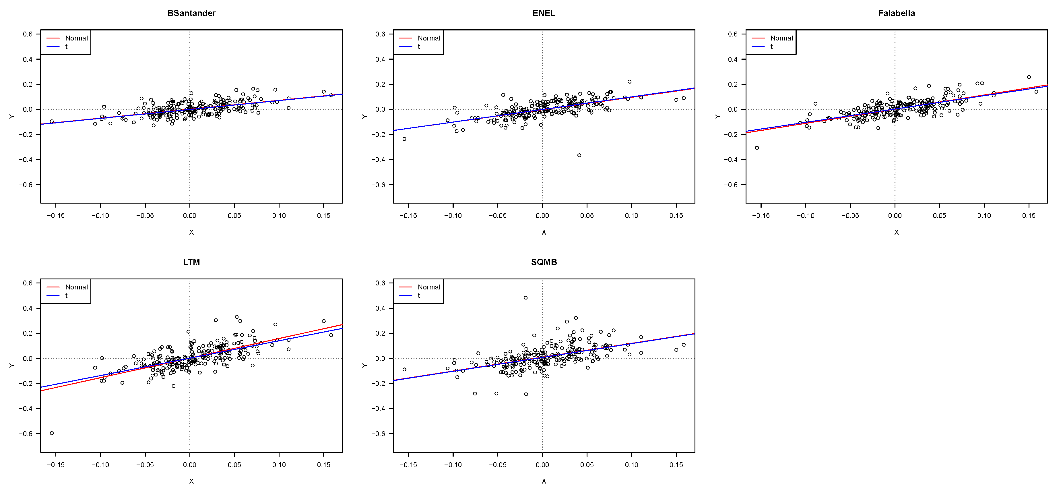
Figure 1 shows scatter plots and estimated lines for the five assets, using the normal and t distributions. From this figure, it is possible to observe linear relationships between asset returns and IPSA returns, and potential outliers. The IPSA index returns explained between 28% and 51% of the variability of the five assets returns. The IPSA index explained 50.94% of the variability in the returns of the Falabella and 27.82% of the returns variability of SQMB.

We also performed an analysis of the heteroscedasticity and autocorrelation of the returns of the five assets. Using the White test (see Lee 1991; Waldman 1983; White 1980) Falabella and LTM showed evidence of heteroscedasticity, while the Durbin-Watson test indicated evidence of first order autocorrelation only in the returns of LTM. Then, considering the significant departure from normality, high kurtosis (evidence that the returns had fat-tailed distributions), the moderate skewness, and the results of the tests for heteroscedasticity and autocorrelation of errors, it is assumed in this study that the random vectors $\{{\mathit{ϵ}}_t,t=1,\dots ,n\}$ were iid as a multivariate t-distribution, with zero mean and covariance matrix $\mathsf{\Sigma }$ and density given by (4). For illustrative purposes, the normal distribution and tests based on weaker distributional assumptions were used, such as the GMM tests, for testing hypothesis (3).

Table 2. Adjustment results of Capital Asset Pricing Model (CAPM) using the multivariate normal and t distributions, standard errors are in parentheses, for the Chilean Stock Market data set.

Model	Asset	$\widehat{\mathit{\alpha }}$	$\widehat{\mathit{\beta }}$			$\widehat{\mathsf{\Sigma }}$
Normal	BSantander	0.0007 (0.0032)	0.7105 (0.0685)	0.0021	−0.0001	−0.0003	−0.0001	−0.0003
	ENEL	−0.0028 (0.0038)	0.9901 (0.0830)		0.0030	−0.0003	0.0004	−0.0005
	Falabella	0.0014 (0.0035)	1.1298 (0.0767)			0.0026	−0.0001	−0.0007
	LTM	0.0019 (0.0052)	1.5608 (0.1124)				0.0056	−0.0004
	SQMB	0.0091 (0.0057)	1.1047 (0.1231)					0.0067
$\mathit{t}(\widehat{\eta }=0.135)$	BSantander	−0.0011 (0.0031)	0.7090 (0.0675)	0.0024	0.0000	−0.0003	−0.0001	−0.0001
	ENEL	−0.0010 (0.0032)	1.0039 (0.0700)		0.0026	−0.0004	0.0002	−0.0006
	Falabella	0.0026 (0.0034)	1.0623 (0.0727)			0.0028	−0.0004	−0.0003
	LTM	0.0014 (0.0047)	1.3873 (0.1011)				0.0054	−0.0002
	SQMB	0.0070 (0.0050)	1.1039 (0.1072)					0.0060

presents the ML estimate for parameters of the CAPM using the normal and t distributions. The standards errors were estimated using the expected information matrix. The results in Table 2 show that the estimates of the coefficients $\alpha$ and $\beta$ were very similar using both models (NCAPM and TCAPM), especially the systematic risk estimators ($\widehat{\beta }$) of the assets considered.

The following hypothesis test $H_0:\eta =0\mathrm{against}{H}_1:\eta >0$ was considered. In this case, it was found that $\widehat{\eta }=0.134926$. The asymptotic distribution of the LR test for the previous hypothesis corresponded to a 50:50 mixture of chi-squares with zero and one degree of freedom, whose critical value was 2.7055 at a significance level of 5% (see, for instance Song et al. 2007). In this case, the maximum log-likelihood for the NCAPM was 1481.39 and for the TCAPM, the maximum log-likelihood was 1524.06, which corresponded to a likelihood-ratio statistic of 85.34. This indicates that the TCAPM fit the data significantly better than the NCAPM. As suggested by a referee, for address the impact of finite samples on the p-values and on the standard errors of the parameter estimates, we also used a nonparametric bootstrap procedure (Chou and Zhou 2006; Efron and Tibshirani 1993). Nevertheless, the results were very similar to those obtained using the normal and t-distribution; therefore, they are not shown here. 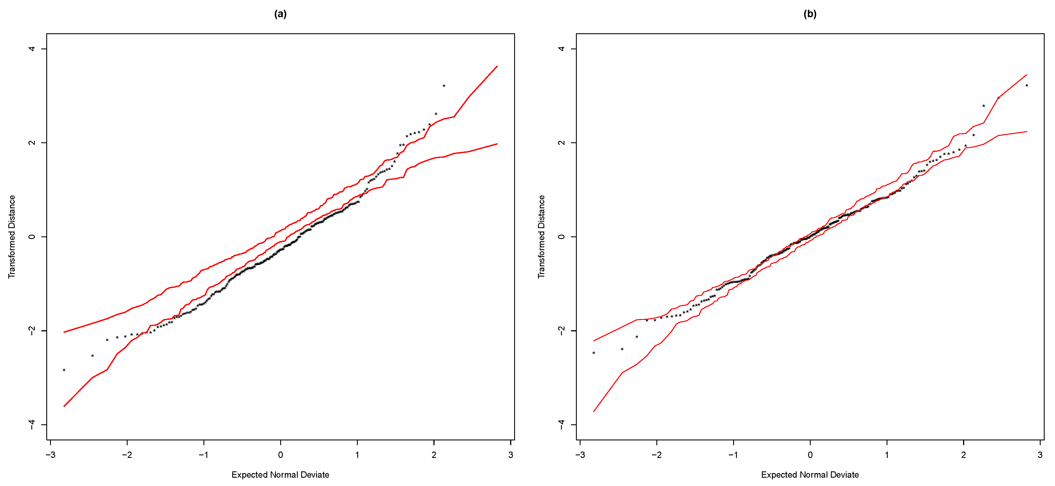Figure 2 displays the transformed distance plots for the normal and t distributions, see Equation (12). These graphics confirm that the TCAPM presented the best fit.

Table 3. Test of the mean-variance efficiency; p-values in parentheses, for the Chilean Stock Market data set.

Test	Normal Fit	Multivariate t Fit	GMM Fit
Wald	3.7243	3.0368	3.6917
	(0.5898)	(0.6943)	(0.5946)
Likelihood-ratio	3.6918	2.9712	-
	(0.5946)	(0.7044)	-
Score	3.6597	2.9508	-
	(0.5994)	(0.7076)	-
Gradient	-	2.9698	-
	-	(0.7046)	-

presents tests results for hypothesis (3) based on the Wald, likelihood-ratio, score, and gradient tests. The results in Table 3 show that the mean-variance efficiency of the IPSA index is not rejected $(p-\mathrm{values}>0.59)$, with any of the tests used for the three scenarios (normal, t-distributions and the GMM).

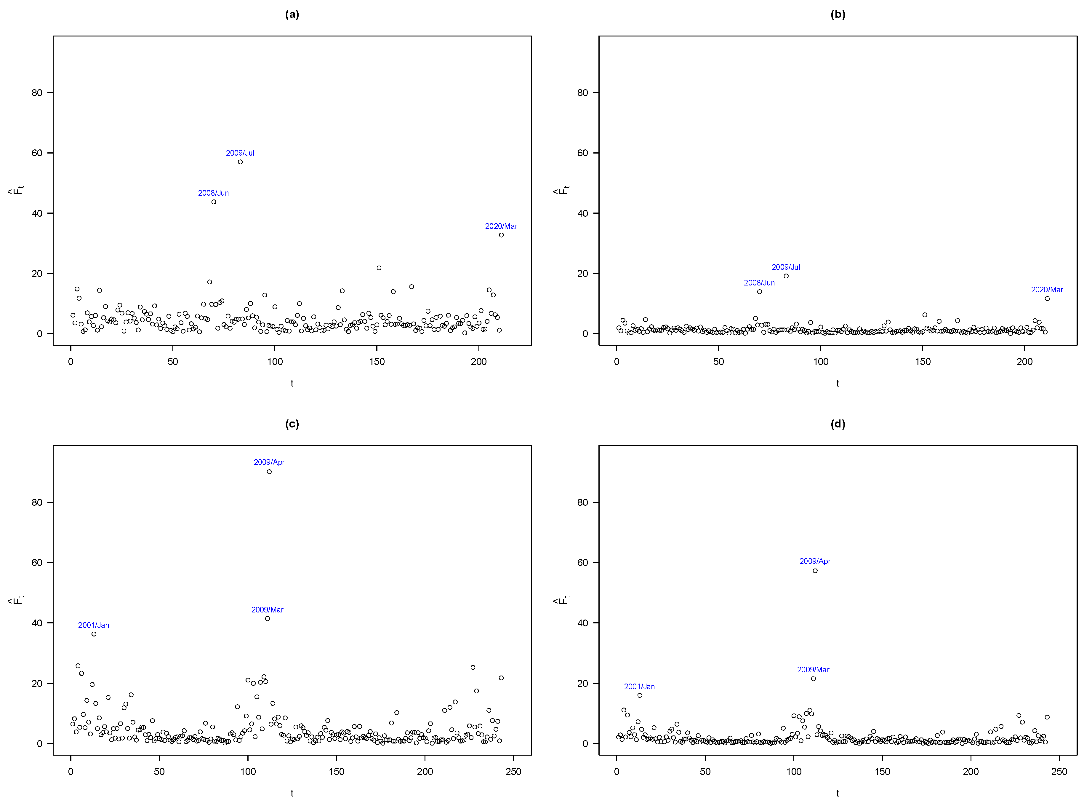
Figure 3 shows the Mahalanobis distances for the normal and t-distribution, for both data sets; the Chilean data set and the New York Stock Exchange data set. For the Chilean data set, under normality Figure 3a, we observe that the returns for 2008/Jun, 2009/Jul and 2020/Mar are possible outliers. For instance, in 2009/Jul, economic activity fell by 3.5%, when Chile entered a recession due to the global financial crisis, while in 2020/Mar, the fall in economic activity (initial) was due to the pandemic caused by Covid-19. Already in Figure 3b, we see as expected, that the TCAPM reduced the possible effect of these returns.

3.2. The New York Stock Exchange Data Set

We considered monthly returns of shares from five companies whose common stock shares trade on the New York Stock exchange, NYSE: Bank of America, Boeing, Ford Motor Company, General Electric Company and Microsoft. The S&P500 was taken as the market price. The 10-year bond yield was used as the risk-free returns; it is a long risk-free rate, similar to the one used for the Chilean data set. The excess returns were the returns minus the risk-free rate. The data corresponded to the period from January, 2000 to March, 2020.

The means, standard deviations (SD), Sharpe ratios (Sharpe), coefficients of skewness and kurtosis, and the Jarque-Bera test (JB Test) for normality of the monthly returns are presented in

Table 4. Summary statistics for monthly log-returns of five assets and S&P500 index from the NYSE data set. p-values are in parentheses.

Asset	Mean (%)	SD (%)	Sharpe	Skewness	Kurtosis	JB Test
Bank of America	−0.0691	11.9324	−0.0281	−1.3041	12.6330	1008.4271
						(0.0000)
Boeing	0.5269	9.2462	0.0282	−1.8571	12.0454	968.1001
						(0.0000)
Ford	−0.7582	13.0995	−0.0782	0.0119	16.1538	1751.8490
						(0.0000)
Gelectric	−0.7728	8.5741	−0.1212	−0.6836	5.9354	106.1649
						(0.0000)
Microsoft	0.4093	8.3394	0.0171	−0.3767	6.7068	144.8702
						(0.0000)
S&P500	0.2300	4.3400	−0.0077	−0.8143	4.4698	48.7262
						(0.0000)

. Boeing had the highest mean return (0.53% per month), while General Electric Company had the lowest average return (−0.77%). In addition, Ford had the highest volatility (13.10%), while Microsoft had the lowest volatility (8.34%) among the five assets. Furthermore, the S&P500 index had a standard deviation of 4.34%, which was less than the volatility of the five assets considered. With the exception of General Electric Company, with a negative Sharpe ratio, the other Sharpe ratios were close to zero.

The assets had a moderate (positive and negative) asymmetry. Again, the returns of the assets had a highest kurtosis. The normality hypothesis was rejected in all the assets using the Jarque-Bera test (JB Test). In brief, the descriptive statistics summary reported in Table 4, confirmed the presence of low levels of skewness and high levels of kurtosis.

Figure 4 shows scatter plots and estimated lines of the five assets, using the normal and t distributions. From this figure, it is possible to observe linear relationships between asset returns and S&P500 returns, and potentials outliers. In this case, the S&P500 index returns explained between 27% and 45% of the variability of the five assets returns, similar to the Chilean Data Set.

The Whites test show evidence of heteroscedasticity in Bank of America, Boeing and Ford Motor Company. The Durbin-Watson test indicates no evidence of first order autocorrelation.

Table 5. Adjustment results of CAPM using the multivariate normal and t distributions, standard errors are in parentheses, for the NYSE data set.

Model	Assets	$\widehat{\mathit{\alpha }}$	$\widehat{\mathit{\beta }}$			$\widehat{\mathsf{\Sigma }}$
Normal	Bank of Am	0.0025 (0.0060)	1.5633 (0.1407)	0.0087	0.0002	0.0019	0.0013	−0.0004
	Boeing	0.0060 (0.0046)	1.1405 (0.1080)		0.0051	0.0007	0.0005	−0.0012
	Ford	−0.0026 (0.0077)	1.7125 (0.1802)			0.0143	0.0006	−0.0005
	Gelectric	−0.0076 (0.0040)	1.3070 (0.0931)				0.0038	−0.0003
	Microsoft	0.0042 (0.0043)	1.1518 (0.1013)					0.0045
$\mathit{t}(\widehat{\eta }=0.277)$	Bank of Am	−0.0017 (0.0044)	1.2387 (0.1036)	0.0087	0.0002	0.0008	0.0007	−0.0004
	Boeing	0.0065 (0.0039)	1.0935 (0.0908)		0.0067	0.0010	0.0004	−0.0011
	Ford	−0.0147 (0.0050)	1.4773 (0.1174)			0.0111	−0.0002	−0.0005
	Gelectric	−0.0074 (0.0032)	1.2406 (0.0747)				0.0045	0.0002
	Microsoft	0.0007 (0.0034)	1.1487 (0.0797)					0.0051

presents the ML estimate for parameters of the CAPM using the normal and t distributions. The standards errors were estimated using the expected information matrix. Similar results to the Chilean data set were observed. For this data set, it was found that $\widehat{\eta }=0.276870,$ indicating a greater departure from normality than the Chilean data set. The likelihood-ratio statistic value, for the hypothesis $H_0:\eta =0\mathrm{against}{H}_1:\eta >0$ was 285.8, which was highly significant. In this case, the maximum log-likelihood for the NCAPM was 1361.2 and for the TCAPM was 1504.1. 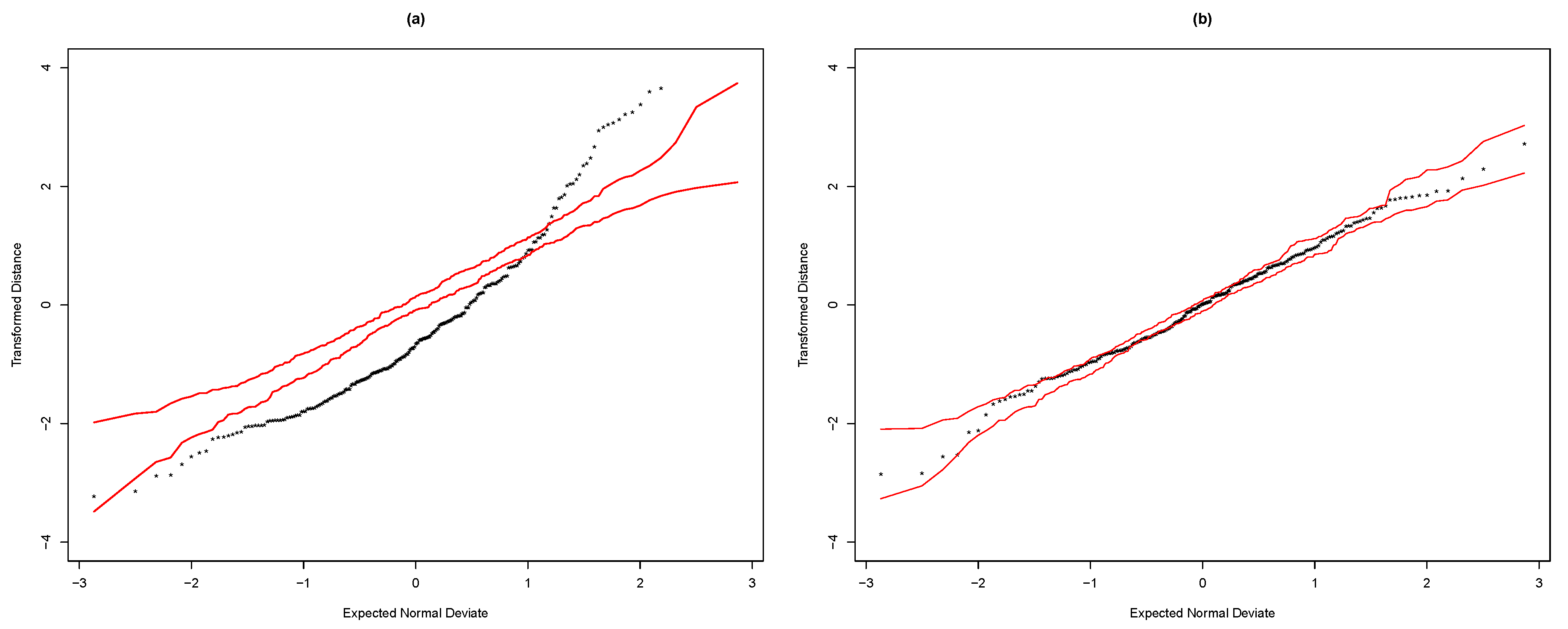Again, this indicates that the TCAPM fit the data significantly better than the NCAPM. This was also confirmed by the transformed distance plots displayed in Figure 5.

Table 6. Test of the mean-variance efficiency; p-values in parentheses, for the NYSE data set.

Test	Normal Fit	Multivariate t Fit	GMM Fit
Wald	8.5507	19.7321	8.5664
	(0.1284)	(0.0014)	(0.1277)
Likelihood-ratio	8.4037	18.7816	-
	(0.1353)	(0.0021)	-
Score	8.2601	18.1012	-
	(0.1425)	(0.0028)	-
Gradient	-	17.9527	-
	-	(0.0030)	-

presents tests results for hypothesis (3). The results in Table 6 show that the mean-variance efficiency of the S&P500 index could not be rejected $(p-\mathrm{values}>0.1277)$, with any of the tests, if we used the NCAPM (or GMM test). However, if we used TCAPM, the hypothesis (3) was rejected $(0.0014<p-\mathrm{values}<0.0030)$ with any of the four tests. That is to say, there was a change in statistical inference.

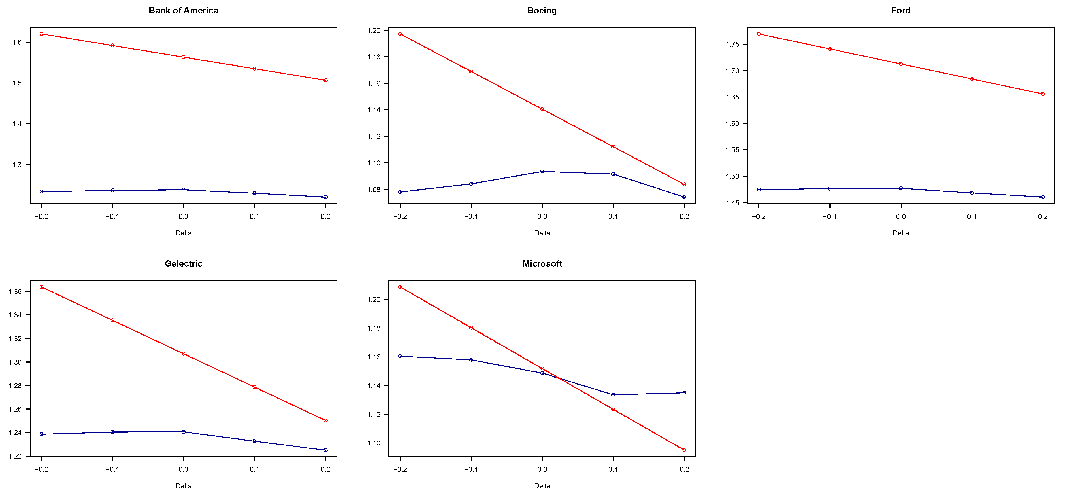
As suggested by a referee, it may also be of interest to test the hypotheses $H_{\beta }:\mathit{\beta }=\mathbf{1}$ and $H_{\alpha \beta }:\mathit{\alpha }=\mathbf{0},\mathit{\beta }=\mathbf{1}$. The four tests were implemented to verify these hypotheses using the t-distribution, see Appendix C. However, with the four tests statistics, we strongly rejected the null hypotheses, and therefore they are not shown in the present study. More details about this interesting topic can be found at Glabadanidis (2009, 2014, 2019).

Figure 3 show the Mahalanobis distances for the NCAPM and TCAPM models, showing results similar to the Chilean data set, except that the return corresponding to 2009/Apr for TCAPM (see Figure 3d) was a possible outlier. In April 2009, the five assets had high returns, highlighting Ford Motor Company, with a 127.4%. However, when deleting these returns, there were no changes in statistical inference. Once again, this suggests that the TCAPM provided an appropriate way for achieving robust inference.

3.3. Robustness

Aspects of the robustness of the TCAPM with respect to the NCAPM can be illustrated perturbing some observations in the original data. Changes in the ML estimates of $\mathit{\beta }$ can be evaluated using the following procedure. First, an observation can be perturbed to create an outlier by ${\mathit{y}}_n\leftarrow {\mathit{y}}_n+\mathsf{\Delta }{\mathbf{1}}_p$, for $\mathsf{\Delta }=-0.20,-0.10,0,0.10,0.20$. Then, we re-calculate the ML estimates of $\mathit{\beta }$ under the TCAPM and under the NCAPM. Note that, for the NCAPM,

$${\widehat{\beta }}_{\mathsf{\Delta }j}={\widehat{\beta }}_j+(x_n-\overline{x})\mathsf{\Delta }/\sum _{t=1}^n{(x_t-\overline{x})}^2,$$

(14)

for $j=1,\dots ,p$. Finally, a graph of ${\widehat{\beta }}_{\mathsf{\Delta }j}$, $j=1,\dots ,p$ versus $\mathsf{\Delta }$ for each of the p assets, is useful to visualize changes in the estimators. Figure 6 and Figure 7 show the curves of the estimates of ${\widehat{\beta }}_{\mathsf{\Delta }j}$, $j=1,\dots ,5$ versus $\mathsf{\Delta }$ for each of the 5 assets included in the two data sets considered in this paper. For this perturbation scheme, it can be observed that the influence on parameter estimation was unbounded in the NCAPM, see Equation (14), whereas it was obviously bounded in the TCAPM. This suggests that TCAPM provided an appropriate way for achieving robust statistical inference.

4. Multifactor Asset Pricing Models under the $\mathit{t}$-Distribution

As suggested by a referee, in some cases it is necessary to use more than one factor to estimate the expected returns of the assets of interest. In this Section we briefly discuss an extension of the TCAPM that includes more than one factor. More details on estimation, hypothesis testing, and applications will be discussed in a separate paper. The multifactor model (MAPM) is a multivariate linear regression model with excess returns on p assets, as follows:

$${\mathit{y}}_t=\mathit{\alpha }+{\mathit{\beta }}_1{x}_{t1}+\dots +{\mathit{\beta }}_q{x}_{tq}+{\mathit{ϵ}}_t,t=1,\dots ,n,$$

(15)

where $(x_1,\dots ,x_q)$ denotes the excess returns of q factors (benchmark assets), ${\mathit{\beta }}_j$ is a $p\times 1$ parameter vector, $j=1,\dots ,q$. The above regression model can be expressed as

$$\begin{array}{ccc}\hfill {\mathit{y}}_t& =& \mathit{\alpha }+{\mathit{B}}_1{\mathit{x}}_t^f+{\mathit{ϵ}}_t,\hfill \\ \hfill {\mathit{y}}_t& =& \mathit{B}{\mathit{x}}_t+{\mathit{ϵ}}_t,\hfill \end{array}$$

(16)

where $\mathit{B}=(\mathit{\alpha },{\mathit{B}}_1)$, denotes the matrix $(p\times q+1)$ of regression coefficients, ${\mathit{B}}_1=({\mathit{\beta }}_1,\dots ,{\mathit{\beta }}_q)$, ${\mathit{x}}_t={(1,{\mathit{x}}_t^f)}^T$ and ${\mathit{x}}_t^f={(x_{t1},\dots ,x_{tq})}^T$, $t=1,\dots ,n.$

As in Section 2.1, we assume that the excess returns ${\mathit{y}}_t$ follows an multivariate t-distribution with mean vector ${\mathit{\mu }}_t$ and variance-covariance matrix $\mathsf{\Sigma }$, named ${\mathit{y}}_t\sim T_p({\mathit{\mu }}_t,\mathsf{\Sigma },\eta )$, independent, $t=1,\dots ,n$, whose density function takes the form,

$$f\left({\mathit{y}}_t\right|\mathit{\theta })={\left|\mathsf{\Sigma }\right|}^{-1/2}g\left({\delta }_t\right),$$

(17)

where, ${\delta }_t={({\mathit{y}}_t-{\mathit{\mu }}_t)}^T{\mathsf{\Sigma }}^{-1}({\mathit{y}}_t-{\mathit{\mu }}_t)$ is the square of the Mahalanobis distance, with ${\mathit{\mu }}_t=\mathit{B}{\mathit{x}}_t$, ${\mathit{x}}_t={(1,x_{t1},\dots ,x_{tq})}^T$ denoting the $t$-th row of the matrix $(n\times q+1)$$\mathit{X}={({\mathit{x}}_1,\dots ,{\mathit{x}}_n)}^T$, for $t=1,\dots ,n$.

Thus, in this case, the ML estimates of B, $\mathsf{\Sigma }$ and $\eta$ are obtained as solution of the following equations (see Equation (9)):

$${\widehat{\mathit{B}}}^T={\left({\mathit{X}}^T\mathit{W}\mathit{X}\right)}^{-1}{\mathit{X}}^T\mathit{W}\mathit{Y},\widehat{\mathsf{\Sigma }}=\frac{1}{n}\sum _{t=1}^n{\omega }_t{\widehat{\mathit{ϵ}}}_t{\widehat{\mathit{ϵ}}}_t^T,$$

(18)

and

$${\widehat{\eta }}^{-1}=\frac{2}{a+loga-1}+0.416\left\{1+erf\left(0.6594log\left(\frac{2.1971}{a+loga-1}\right)\right)\right\},$$

where ${\widehat{\mathit{ϵ}}}_t={\mathit{y}}_t-{\widehat{B}}^T{x}_t$ and $W=\mathrm{diag}({\omega }_1,\dots ,{\omega }_n)$ an $n\times n$ diagonal matrix with elements ${\omega }_t=\left({\displaystyle \frac{1+\eta p}{\eta }}\right)\left({\displaystyle \frac{c\left(\eta \right)}{1+c\left(\eta \right){\delta }_t}}\right)$, for $t=1,\dots ,n$, and the matrix $(n\times p)$$\mathit{Y}={({\mathit{y}}_1,\dots ,{\mathit{y}}_n)}^T$.

As in Section 2.3, the standard errors of the ML estimators $\widehat{\mathit{B}}$, $\widehat{\mathsf{\Sigma }}$ and $\widehat{\eta }$ can be estimated using the expected information matrix. In this case, the Fisher information matrix for $\mathit{\theta }=(\mathit{B},\mathsf{\Sigma },\eta )$ assumes the same form of the matrix J given in the Equation (10), but the information concerning to B is now ${\mathit{J}}_{11}=c_{\alpha }\left(\eta \right)\left({\mathit{X}}^T\mathit{X}\right)\otimes {\mathsf{\Sigma }}^{-1}$, with $c_{\alpha }$ as defined in Equation (10). To test linear hypotheses of interest, such as $H_{\alpha }$, we can use the same four tests discussed in Section 2.4.

As a illustration we consider the NYSE data set. We fit the following three-factor model,

$${\mathit{y}}_t=\mathit{\alpha }+{\mathit{\beta }}_1{x}_t+{\mathit{\beta }}_2{\mathrm{SMB}}_t+{\mathit{\beta }}_3{\mathrm{HML}}_t+{\mathit{ϵ}}_t,k=1,\dots ,n,$$

(19)

where, x is the excess return of the S&P500 index, used in the NYSE data set, while SMB and HML used in the Fama-French model were from the website of Prof. Kenneth French. For details on risk factors, SMB and HML see Fama and French (1995).

In this case, the three risk factors explained between 32% and 50% of the variability of the five assets’ returns, which corresponded to an increase of approximately 5% with respect to the CAPM. From

Table 7. Adjustment results of Multifactor Asset Pricing Model (MAPM) using the multivariate normal and t distributions from the NYSE data set and Fama-French data set. Standard errors are in parentheses.

Model	Asset	$\widehat{\mathit{\alpha }}$	${\widehat{\mathit{\beta }}}_1$	${\widehat{\mathit{\beta }}}_2$	${\widehat{\mathit{\beta }}}_3$
Normal	Bank of Am	0.0006 (0.0052)	1.4698 (0.1237)	0.2059 (0.1656)	1.4310 (0.1624)
	Boeing	0.0052 (0.0044)	1.1015 (0.1042)	0.0557 (0.1395)	0.6612 (0.1367)
	Ford	−0.0041 (0.0075)	1.6341 (0.1765)	0.3050 (0.2363)	0.9135 (0.2317)
	Gelectric	−0.0081 (0.0038)	1.2836 (0.0910)	−0.0050 (0.1218)	0.4815 (0.1194)
	Microsoft	0.0051 (0.0041)	1.1967 (0.0970)	−0.1058 (0.1298)	−0.6713 (0.1273)
$t(\widehat{\eta }=0.27)$	Bank of Am	−0.0017 (0.0027)	1.1916 (0.0634)	0.1535 (0.0849)	1.2474 (0.0832)
	Boeing	0.0056 (0.0026)	1.1063 (0.0609)	−0.0279 (0.0815)	0.5455 (0.0799)
	Ford	−0.0149 (0.0033)	1.4170 (0.0780)	0.2127 (0.1045)	0.6901 (0.1024)
	Gelectric	−0.0081 (0.0021)	1.2611 (0.0497)	−0.1479 (0.0665)	0.3387 (0.0652)
	Microsoft	0.0017 (0.0022)	1.1636 (0.0524)	−0.3077 (0.0701)	−0.4498 (0.0688)

, wecan see that the values in $\widehat{\mathit{\alpha }}$ were very similar to those obtained using CAPM as presented in Table 5, while estimates in ${\widehat{\mathit{\beta }}}_1$ tended to be lower than estimates in $\widehat{\mathit{\beta }}$, in the case of CAPM (see Table 5).

Figure 8 displays the transformed distance plots for the normal and t distributions. Here NMAPM denotes the three risk factors under normality and TMAPM denotes the three risk factors under multivariate t-distribution. These graphics show clear evidence that the TMAPM had a better fit than the NMAPM. Using the likelihood-ratio test, the hypothesis $H_{\alpha }$ could not be rejected $(p-\mathrm{value}=0.1277)$, if we used the NMAPM. However, if we used TMAPM, the hypothesis (3) was rejected $(p-\mathrm{value}=0.0011)$. Once again, there was a change in statistical inference.

5. Conclusions

Since the pioneering work by Lange et al. (1989), the t-distribution has proved to be a versatile and robust modeling approach in many regression models. In fact, the t-distribution has a parameter ($\eta$) modeling kurtosis, which brings more flexibility than the normal distribution.

In this paper, robust methods for statistical inference in asset pricing models with emphasis on CAPM were developed. In effect, assuming a multivariate t-distribution for the stock returns, ML equations for parameters were derived and statistics were proposed to test linear hypotheses of interest, in particular the hypothesis of mean-variance efficiency. Simple expressions were provided in this study for the likelihood-ratio, Wald, score and gradient statistics and for the score function and Fisher information matrix. The proposed statistics generalized results from the literature, which considered tests for mean-variance efficiency under the assumption of multivariate normality (Brandimarte 2018; Campbell et al. 1997; Chou and Lin 2002; Gibbons et al. 1989; Mazzoni 2018). In addition, statistical inference based on the t-distribution is simple to implement, and the computational cost is considerably low.

A simple graphical device for checking the model was implemented, and the methodology developed in this paper was illustrated with two real data sets: the Chilean Stock Market data set (a developing country), and another from the New York Stock Exchange, USA (a developed country). In both data sets, the CAPM under the t-distribution clearly presents a better fit than under the normal distribution. Additionally, in the application of the multifactor asset pricing model to the NYSE data set, the multivariate t-distribution presents a better fit than the normal distribution.

This empirical study provides new evidence for the useful application of the t-distribution in modeling stock returns (Kan and Zhou 2017). As we have pointed out, the log-returns frequently present some degree of skewness. We are currently working on statistical inference in the asset pricing models under the multivariate skew-elliptical distributions. We understand that a skewed t-distribution of Branco and Dey (2001) may be useful for returns with high levels of skewness. For previous applications of the skew-elliptical distributions in finance and actuarial science, see Harvey et al. (2010) and Adcock et al. (2015). See also Paula et al. (2011).

References

1. Adcock, Christopher, Martin Eling, and Nicola Loperfido. 2015. Skewed distributions in finance and actuarial science: A review. The European Journal of Finance 21: 1253–81. [Google Scholar] [CrossRef]
2. Amenc, Noel, and Veronique Le Sourd. 2003. Portfolio Theory and Performance Analysis. New York: John Wiley. [Google Scholar]
3. Barillas, Francisco, and Jay Shanken. 2018. Comparing Asset Pricing Models. The Journal of Finance 73: 715–54. [Google Scholar] [CrossRef] [Green Version]
4. Bao, Te, Ceer Diks, and Hao Li. 2018. A generalized CAPM model with asymmetric power distributed errors with an application to portfolio construction. Economic Modelling 68: 611–21. [Google Scholar] [CrossRef]
5. Bekaert, Geer, and Guojun Wu. 2000. Asymmetric Volatility and Risk in Equity Markets. The Review of Financial Studies 13: 1–42. [Google Scholar] [CrossRef] [Green Version]
6. Berk, Jonathan. 1997. Necessary conditions for the CAPM. Journal of Economic Theory 73: 245–57. [Google Scholar] [CrossRef] [Green Version]
7. Blattberg, Robert C., and Nicholas J. Gonedes. 1974. A comparison of the stable and student distribution as statistical models for stock prices. Journal of Business 47: 244–80. [Google Scholar] [CrossRef]
8. Bolfarine, Heleno, and Manuel Galea. 1996. On structural Comparative Calibration under a t-model. Computational Statistics 11: 63–85. [Google Scholar]
9. Boos, Dannis D., and Leonard A. Stefanski. 2013. Essential Statistical Inference, Theory and Methods. New York: Springer. [Google Scholar]
10. Borup, Daniel. 2019. Asset pricing model uncertainty. Journal of Empirical Finance 54: 166–89. [Google Scholar] [CrossRef]
11. Branco, Marcia D., and Dipak K. Dey. 2001. A general class of multivariate skew-elliptical distributions. Journal of Multivariate Analysis 79: 99–113. [Google Scholar] [CrossRef] [Green Version]
12. Brandimarte, Paolo. 2018. An Introduction to Financial Markets: A Quantitative Approach. Hoboken: John Wiley. [Google Scholar]
13. Broquet, Claude, Robert Cobbaut, Roland Gillet, and Andre van den Berg. 2004. Gestion de Portefeuille, 4th ed. Louvain-la-Neuve: De Boeck Université. Bruxelles. [Google Scholar]
14. Cademartori, David, Cecilia Romo, Richardo Campos, and Manuel Galea. 2003. Robust estimation of systematic risk using the t-distribution in the Chilean Stock Markets. Applied Economics Letters 10: 447–53. [Google Scholar] [CrossRef]
15. Campbell, John, Andrew Lo, and A. Craig MacKinlay. 1997. Econometrics of Financial Markets. Princeton: Princeton University Press. [Google Scholar]
16. Chamberlain, Gary. 1983. A characterization of the distributions that imply mean-variance utility functions. Journal of Economic Theory 29: 185–201. [Google Scholar] [CrossRef]
17. Chen, Joseph, Harrison Hong, and Jeremy C. Stein. 2001. Forecasting crashes: Trading volume, past returns, and conditional skewness in stock prices. Journal of Financial Economics 61: 345–81. [Google Scholar] [CrossRef] [Green Version]
18. Chou, Pin-Huang, and Mei-Chen Lin. 2002. Tests of international asset pricing model with and without a riskless asset. Applied Financial Economics 12: 873–83. [Google Scholar] [CrossRef]
19. Chou, Ping-Huang, and Guofu Zhou. 2006. Using Bootstrap to Test Portfolio Efficiency. Annals of Economics and Finance 2: 217–49. [Google Scholar]
20. Efron, Bradley, and Robert J. Tibshirani. 1993. An Introduction to the Bootstrap. New York: Chapman and Hall. [Google Scholar]
21. Ejara, Demissew, Alain Krapl, Thomas J. O’Brien, and Santiago Ruiz de Vargas. 2019. Local, Global, and International CAPM: For Which Countries Does Model Choice Matter? Available online: https://ssrn.com/abstract=3023501 (accessed on 24 January 2020).
22. Elton, Edwin, and Martin Gruber. 1995. Modern Portfolio Theory and Investment Analysis. New York: John Wiley. [Google Scholar]
23. Fama, Eugene. 1965. The behavior of stock market prices. Journal of Business 38: 34–105. [Google Scholar] [CrossRef]
24. Fama, Eegene, and Kenneth R. French. 1995. Size and book-to-market factors in earnings and returns. Journal of Finance 50: 131–55. [Google Scholar] [CrossRef]
25. Fiorentini, Gabriele, Enriques Sentana, and Giorgio Calzolari. 2003. Maximum likelihood estimation and inference in multivariate conditionally heteroscedastic dynamic regression models with Student t innovations. Journal of Business & Economic Statistics 21: 532–46. [Google Scholar]
26. Francis, Jack Clark, and Dongcheol Kim. 2013. Modern Portfolio Theory: Foundation, Analysis, and New Dvelopments. Hoboken: John Wiley. [Google Scholar]
27. Galea, Manuel, Jose A. Díaz-Garcá, and Filidor Vilca. 2008. Influence diagnostics in the capital asset pricing model under elliptical distributions. Journal of Applied Statistics 35: 179–92. [Google Scholar] [CrossRef]
28. Galea, Manuel, David Cademartori, and Filidor Vilca. 2010. The structural sharpe model under t-distributions. Journal of Applied Statistics 37: 1979–90. [Google Scholar] [CrossRef]
29. Galea, Manuel, and Patricia Giménez. 2019. Local influence diagnostics for the test of mean-variance efficiency and systematic risks in the Capital Asset Pricing Model. Statistical Papers 60: 293–312. [Google Scholar] [CrossRef]
30. Gibbons, Michael, Stephen Ross, and Jay Shanken. 1989. A test of the efficiency of a given portfolio. Econometrica 57: 1121–53. [Google Scholar] [CrossRef] [Green Version]
31. Glabadanidis, Paskalis. 2009. Measuring the economic significance of mean-variance spanning. The Quarterly Review of Economics and Finance 49: 596–616. [Google Scholar] [CrossRef]
32. Glabadanidis, Paskalis. 2014. What Difference Fat Tails Make: A Bayesian MCMC Estimation of Empirical Asset Pricing Models. In Bayesian Inference in the Social Sciences. Edited by Ivan Jeliazkov and Xin-She Yang. Hoboken: John Wiley. [Google Scholar]
33. Glabadanidis, Paskalis. 2019. An exact test of the improvement of the minimum variance portfolio. International Review of Finance 19: 45–82. [Google Scholar] [CrossRef] [Green Version]
34. Hamada, Mahmoud, and Emiliano A. Valdez. 2008. CAPM and option pricing with elliptically contoured distributions. The Journal of Risk and Insurance 75: 387–409. [Google Scholar] [CrossRef]
35. Hansen, Lars Peter. 1982. Large Sample Properties of Generalized Method of Moments Estimators. Econometrica 50: 1029–54. [Google Scholar] [CrossRef]
36. Harvey, Campbell, and Guofu Zhou. 1993. International asset pricing with alternative distributional specifications. Journal of Empirical Finance 1: 107–31. [Google Scholar] [CrossRef] [Green Version]
37. Harvey, Campbell R., John Liechty, M. Liechty, and P. M. Müller. 2010. Portfolio selection with higher moments. Quantitative Finance 10: 469–85. [Google Scholar] [CrossRef]
38. Hodgson, Douglas, Oliver Linton, and Keith Vorkink. 2002. Testing the capital asset pricing model efficiently under elliptical symmetry: A semiparametric approach. Journal of Applied Econometrics 17: 617–39. [Google Scholar] [CrossRef] [Green Version]
39. Ingersoll, Jonathan. 1987. Theory of Financial Decision Making. Lanham: Rowman and Littlefield. [Google Scholar]
40. Johnson, R. Stafford. 2014. Equity Markets and Portfolio Analysis. Hoboken: John Wiley. [Google Scholar]
41. Kan, Raymond, and Guofu Zhou. 2017. Modeling Non-normality Using Multivariate t: Implications for Asset Pricing. China Finance Review International 7: 2–32. [Google Scholar] [CrossRef] [Green Version]
42. Lange, Kenneth L., Roderick J. Little, and Jeremy Taylor. 1989. Robust statistical modelling using the t-distribution. Journal of the American Statistical Association 84: 881–96. [Google Scholar]
43. Lee, John. 1991. A Lagrange multiplier test for GARCH models. Economics Letters 37: 265–71. [Google Scholar] [CrossRef] [Green Version]
44. Lemonte, Artur. 2016. The Gradient Test: Another Likelihood-Based Test. London: Academic Press. [Google Scholar]
45. Levy, Haim. 2012. The Capital Asset Pricing Model in the 21st Century: Analytical, Empirical, and Behavioral Perspectives. New York: Cambridge University Press. [Google Scholar]
46. Lintner, John. 1965. The valuation of risk assets and the selection of risky investments in stock portfolios and capital budgets. Review of Economics and Statistics 41: 13–37. [Google Scholar] [CrossRef]
47. Liu, Chuanhai, and Donald B. Rubin. 1995. ML estimation of the t distribution using EM and its extensions, ECM and ECME. Statistica Sinica 5: 19–39. [Google Scholar]
48. MacKinlay, A. Craig, and Mathew P. Richardson. 1991. Using Generalized Method of Moments to Test Mean-Variance Efficiency. The Journal of Finance 46: 511–27. [Google Scholar] [CrossRef]
49. Magnus, Jan R., and Heinz Neudecker. 2007. Matrix Differential Calculus with Applications in Statistics and Econometrics, 3rd ed. New York: John Wiley. [Google Scholar]
50. Mazzoni, Thomas. 2018. A First Course in Quantitative Finance. New York: Cambridge University Press. [Google Scholar]
51. Mitchell, Ann. 1989. The information matrix, skewness tensor and α-connections for the general multivariate elliptic distributions. Annals of the Institute of Statistical Mathematics 41: 289–304. [Google Scholar] [CrossRef]
52. Mossin, Jan. 1966. Equilibrium in capital asset market. Econometrica 35: 768–83. [Google Scholar] [CrossRef]
53. Owen, Joel, and Ramon Rabinovitch. 1983. On the class of elliptical distributions and their applications to the theory of portfolio. The Journal of Finance 38: 745–52. [Google Scholar] [CrossRef]
54. Paula, Gilberto, Victor Leiva, Michelli Barros, and Shuangzhe Liu. 2011. Robust statistical modeling using the Birnbaum-Saunders-t distribution applied to insurance. Applied Stochastic Models in Business and Industry 28: 16–34. [Google Scholar] [CrossRef]
55. Pereiro, Luis E. 2010. The beta dilemma in emerging markets. Journal of Applied Corporate Finance 22: 110–22. [Google Scholar] [CrossRef]
56. Pinheiro, Jose C., Chuanhai Liu, and Ying Nian Wu. 2001. Efficient algorithms for robust estimation in linear mixed-effects models using the multivariate t distribution. Journal of Computational and Graphical Statistics 10: 249–76. [Google Scholar] [CrossRef]
57. Sharpe, William. 1964. Capital asset prices: A theory of markets equilibrium under conditions of risk. Journal of Finance 19: 425–42. [Google Scholar]
58. Shoham, Shy. 2002. Robust clustering by deterministic agglomeration EM of mixtures of multivariate t distribution. Pattern Recognition 35: 1127–42. [Google Scholar] [CrossRef]
59. Song, Peter. X. -K., Peng Zhang, and Annie Qu. 2007. Maximum likelihood inference in robust linear mixed-effects models using the multivariate t distributions. Statistica Sinica 17: 929–43. [Google Scholar]
60. Sutradhar, Brajendra C. 1993. Score test for the covariance matrix of elliptical t-distribution. Journal of Multivariate Analysis 46: 1–12. [Google Scholar] [CrossRef] [Green Version]
61. Terrell, George. 2002. The Gradient Statistic. Computing Science and Statistics 34: 206–15. [Google Scholar]
62. Vorkink, Keith. 2003. Return distributions and improved tests of asset pricing models. The Review of Financial Studies 16: 845–74. [Google Scholar] [CrossRef]
63. Waldman, Donald M. 1983. A note on algebraic equivalence of White’s test and a variation of the Godfrey/Breusch-Pagan test for heteroscedasticity. Economics Letters 13: 197–200. [Google Scholar] [CrossRef]
64. White, Halbert. 1980. A Heteroskedasticity-Consistent Covariance Matrix Estimator and a Direct Test for Heteroskedasticity. Econometrica 48: 817–38. [Google Scholar] [CrossRef]
65. Xie, Feng-Chang, Bo-Cheng Wei, and Jin-Guan Lin. 2007. Case-deletion Influence Measures for the Data from Multivariate t Distributions. Journal of Applied Statistics 34: 907–21. [Google Scholar] [CrossRef]
66. Zhou, Guofu. 1993. Asset-pricing test under alternative distributions. The Journal of Finance 48: 1927–42. [Google Scholar] [CrossRef]
Figure 1. Scatter plots and estimated lines for five assets, using the normal and t distributions, for the Chilean Stock Market data set.
Jrfm 13 00123 g001
Figure 2. QQ-plot of transformed distances for the NCAPM (a) and TCAPM (b), for the Chilean Stock Market data set.
Jrfm 13 00123 g002
Figure 3. Mahalanobis distances ( F ^ t ) for the NCAPM (a) and TCAPM (b), for the Chilean Stock Market data set, and NCAPM (c) and TCAPM (d) for the NYSE data set.
Jrfm 13 00123 g003
Figure 4. Scatter plots and estimated lines for five assets, using the normal and t distributions, for the NYSE data set.
Jrfm 13 00123 g004
Figure 5. Plots of transformed distances for the NCAPM (a) and TCAPM (b), for the NYSE data set.
Jrfm 13 00123 g005
Figure 6. Perturbed ML estimates of β under the NCAPM (red line) and TCAPM (blue line), for the Chilean Stock Market data set.
Jrfm 13 00123 g006
Figure 7. Perturbed maximum likelihood (ML) estimates of β under the NCAPM (red line) and TCAPM (blue line), for the NYSE data set.
Jrfm 13 00123 g007
Figure 8. Plots of transformed distances for the NMAPM (a) and TMAPM (b), for the NYSE data set.
Jrfm 13 00123 g008