Article

The Costs and Benefits of Bank Capital—A Review of the Literature †

1
Secretariat of the Basel Committee on Banking Supervision, Bank for International Settlements, CH-4002 Basel, Switzerland
2
Directorate International Economics and Cooperation, Bank of France, 75049 Paris, France
3
Division of Supervision & Regulation, Board of Governors of the Federal Reserve System, Washington, DC 20551, USA
4
Financial Regulations Division, Central Bank of Argentina, Buenos Aires C1003ABF, Argentina
5
Division of Research & Statistics, Board of Governors of the Federal Reserve System, Washington, DC 20551, USA
6
Financial Stability Department, Norges Bank, 0151 Oslo, Norway
7
Financial System Research Division, Bank of Japan, Tokyo 103 8660, Japan
8
Financial Intermediation Function, Federal Reserve Bank of New York, New York, NY 10045, USA
9
Economics Department, Office of the Comptroller of the Currency, Washington, DC 20219, USA
10
Directorate Financial Stability, Bank of France, 75049 Paris, France
11
Prudential Policy Directorate, Bank of England, London EC2R 8AH, UK
*
Author to whom correspondence should be addressed.
The Working Papers of the Basel Committee on Banking Supervision contain analysis carried out by experts of the Basel Committee or its working groups. They may also reflect work carried out by one or more member institutions or by its Secretariat. The subjects of the Working Papers are of topical interest to supervisors and are technical in character. The views expressed in the Working Papers are those of their authors and do not represent the official views of the Basel Committee, its member institutions or the Bank for International Settlements.
J. Risk Financial Manag. 2020, 13(4), 74; https://doi.org/10.3390/jrfm13040074
Submission received: 18 February 2020 / Revised: 24 March 2020 / Accepted: 11 April 2020 / Published: 16 April 2020
(This article belongs to the Section Banking and Finance)

Abstract

:
In 2010, the Basel Committee on Banking Supervision published an assessment of the long-term economic impact (LEI) of stronger capital and liquidity requirements. This paper considers this assessment in light of estimates from later studies of the macroeconomic benefits and costs of higher capital requirements. Consistent with the Basel Committee’s original assessment, this paper finds that the net macroeconomic benefits of capital requirements are positive over a wide range of capital levels. Under certain assumptions, the literature finds that the net benefits of higher capital requirements may have been understated in the original committee assessment. Put differently, the range of estimates for the theoretically optimal level of capital requirements—where marginal benefits equal marginal costs—is likely either similar to, or higher than was originally estimated by the Basel Committee. The above conclusion is however subject to a number of important considerations. First, estimates of optimal capital are sensitive to a number of assumptions and design choices. For example, the literature differs in judgments made about the permanence of crisis effects as well as assumptions about the efficacy of post crisis reforms, such as liquidity regulations and bank resolution regimes, in reducing the probability and costs of future banking crisis. In some cases, these judgements can offset the upward tendency in the range of optimal capital. Second, differences in (net) benefit estimates can reflect different conditioning assumptions such as starting levels of capital or default thresholds (the capital ratio at which firms are assumed to fail) when estimating the impact of capital in reducing crisis probabilities. Finally, the estimates are based on capital ratios that are measured in different units. For example, some studies provide optimal capital estimates in risk-weighted ratios, others in leverage ratios. And, across the risk-weighted ratio estimates, the definition of capital and risk-weighted assets (RWAs) can also differ (e.g., tangible common equity (TCE) or Tier 1 or common equity tier 1 (CET1) capital; Basel II RWAs vs. Basel III measures of RWAs). A full standardisation of the different estimates across studies to allow for all of these considerations is not possible on the basis of the information available and lies beyond the scope of this paper. This paper also suggests a set of issues which warrant further monitoring and research. This includes the link between capital and the cost and probability of crises, accounting for the effects of liquidity regulations, resolution regimes and counter-cyclical capital buffers, and the impact of regulation on loan quantities.

1. Introduction

This report considers the analysis of the assessment by the Basel Committee on Banking Supervision (BCBS) of the long-term economic impact (LEI) of stronger capital and liquidity requirements (BCBS 2010) in light of more recently published analyses. The original LEI analysis weighed the benefits and costs of higher capital requirements:1 the benefits of fewer and less costly crises versus the output drag from higher loan spreads. With that simple stabiliser/drag framing, and postponing details, the net marginal benefits of more bank capital k can be expressed in stylised form as:
Net benefits (k) = reduced crisis probability (k) × crisis cost − output drag (loan spreads (k))
In this approach, more capital k is beneficial as long as the stability benefits of higher capital minus the economic drag (the net benefits) is positive holding all else, including other post-crisis regulations, constant (see Appendix A for a recap of the results in BCBS (2010)). The theoretically-optimal capital ratio, denoted k*, is where the marginal benefit of additional capital equals the marginal costs and net benefits are maximised.
Section 2 discusses how the benefits and costs of higher capital—the components of net benefits above—are estimated and how techniques, data and findings have evolved since BCBS (2010). This section also discusses how some later studies have attempted to incorporate other (non-capital) reforms, namely total loss-absorbing capacity (TLAC) and enhanced resolution strategies, into the optimal capital calculus. In principle, those gone-concern reforms tend to serve to reduce the costs and/or probability of crises and thus, all else equal, lower k*. Until crisis-tested, however, gauging the effect of those reforms on optimal capital is highly uncertain.
An important assumption of the LEI is that the calibration of the optimal level of capital is made holding other regulations constant. While the BCBS (2010) study does make some allowance for liquidity regulation, many of the studies reviewed do not incorporate liquidity requirements (or other post-crisis reforms) into their analysis. This enables a tighter focus on the effects of capital requirements. Naturally, this implies that a separate, more in-depth, analysis of the effects of liquidity regulations and other regulations may prove to be helpful.
Section 3 expands the focus to include findings from a survey of research task force (RTF) members combined with a broader literature survey of “piecemeal” studies that estimate components of the marginal benefits and costs of capital but are not full-fledged, optimal capital studies. New estimates from this literature raise the question of whether the stabilising effect of bank capital operates more from reducing the costs of crisis, rather than their probability.
Section 4 compares estimates of the components of marginal benefits and marginal costs from the LEI analysis, the optimal capital studies discussed in Section 2, and the piecemeal studies discussed in Section 3. We show that k* is likely either similar or higher than was originally estimated by the Committee in 2010. This section also discusses possible improvements to the LEI framework.

2. Basel Committee Long-Term Economic Impact Analysis and Subsequent Studies

The Basel Committee’s 2010 LEI analysis (BCBS 2010) focused on the macroeconomic benefits and costs of higher capital requirements. Subsequent studies have built on the LEI approach to consider optimal capital levels. Table 1 provides a high-level summary of the BCBS (2010) LEI study and eight follow-on studies identified using essentially the same benefit-cost/stabiliser-drag approach to estimating optimal bank capital levels (k*). The list of follow-on studies is not exhaustive. Only studies that explicitly analysed capital benefits and costs at the margin, and thus delivered (or implied) k*, were covered.2 Considerable caution is required in interpreting the table. While the assumptions reported were usually clearly stated in the studies, the marginal benefit and cost estimates were not always as clear, so some inference was required to populate those rows. This is not meant as a criticism of the authors of these studies. In pursuit of robustness and thoroughness, these papers provide myriad model runs under varying assumptions, from which it is difficult to identify the baseline model.
The bottom row reports the range of k* estimates reported or derived from each study. The range is fairly wide across studies, and often within studies, reflecting the considerable uncertainties involved in optimal capital levels and the myriad alternative assumptions and calibrations authors used to mitigate the uncertainties. For example, sample coverage differs, i.e., the LEI covered all BCBS member countries, while most of the recent studies are country-specific. Moreover, the definition of capital ratios can vary: the LEI was based on a mapping of banks’ tangible common equity (TCE) to Basel II risk-weighted assets (RWA) while more recent studies are based on actual Basel III capital ratio data, which hinders comparison.3 Bearing those (and the above) caveats in mind, the k* estimated in later studies is either similar or higher than the estimate in the LEI, but still with a wide range of estimates. Given such uncertainty in modelling k*, the LEI did not advocate in favour of a particular calibration of the requirements, nor does this paper.
Below, we consider the LEI in greater detail and assess how its estimates compare to those in later studies. The review proceeds “horizontally” by the main components of the marginal benefits and costs of bank capital that jointly determine k*. Reviewing horizontally rather than vertically (i.e., by study) better informs an eclectic approach to any future research. We highlight commonalities and divergences in how the LEI and later studies estimated each component, key assumptions, and uncertainties, and discuss important recent studies outside the k* literature that can inform it.

2.1. Stability Benefits of Bank Capital

The LEI and later studies focus on the crisis prevention, versus cost mitigation, benefits of a better capitalised banking system. The estimated marginal reduction in the annual probability of a crisis ranged across studies from as little as 0.03 percentage points to as much as 1.7 percentage points.4 The LEI estimate of 1.6 percentage points reported in Table 1 is near the high end, however as shown in Section 4, these estimate are highly sensitive to the starting capital ratio. The LEI reports a reduction in the probability of crisis by 1.6% when the capital ratio increases from 7% to 8%, abstracting from the additional impact of liquidity regulation, but increasing the capital ratio from 12% to 13% only reduces the crisis probability by 0.2%. This is similar to the range of reported studies in Table 1.
The studies arrive at these estimates using either of two (or both) methods. The “top-down” method uses country level data to estimate the relationship between crisis indicators and banking system capital. The “bottom-up” method estimates the relationship between capital and failure at the bank level and then extrapolates to the banking system/crisis level in various ways. Neither method is necessarily better; top down is simpler and more direct. The bottom-up approach is more micro-founded but involves estimation and simulation. Most studies, including the LEI, use both methods for robustness.
The typical top-down model estimates the probability of a crisis as a function of banking system capital and various financial control variables that might also affect crisis risk:
Probability (crisis) = function (capital, controls)
where crisis is a country level crisis indicator and capital measures banking system capital per assets or RWA. Typical controls include bank liquidity (an indirect attempt to include liquidity regulation in the analysis, see Section 2.2), credit/gross domestic product (GDP), volatility index (VIX), house prices, and trade balance.5 In general, the probability of a crisis is found to decline when banking system capital is higher, though the size and statistical significance of the effect varies across studies.
While the top-down models all control for financial crisis drivers, e.g., credit/GDP, none seem to control for real drivers, such as GDP growth. That is notable, because crises are often preceded by real growth slowdowns which may even “set the stage” for the crisis while at the same time reducing bank capital via lower loan demand and higher loan losses. Omitting real drivers from top-down models may confound the stabilising effect of stronger growth and higher capital (see Appendix B). The bottom-up method involves estimating the distribution of bank-level losses, then using simulations to estimate the probability of such losses reaching crisis levels by depleting banking system capital to crisis proportions. The study by the Federal Reserve Bank of Minneapolis (2017), for example, following Dagher et al. (2016), converts peak nonperforming loans that are sustained in crises to equivalent capital losses, then estimates the marginal benefit of additional capital in averting a crisis or bailout.
The bottom-up approach in Miles et al. (2013) is unusual in that they stipulate a one-to-one positive relationship between bank assets and (permanent) output and then estimate the probability of output shocks sufficient to deplete bank capital and cause substantial bank failures. Their “real only” crisis concept contrasts with the “financial only” concept in the top-down model just noted, as well as the 2007–2009 crisis which clearly had partly financial origins.
Jorda et al. (2017) focus attention on the cost containment benefits of capital rather than the crisis prevention effects. Using bank balance sheet and crisis data from 1870 to 2013 for 17 advanced economies, they conclude that higher bank capital ratios are unlikely to prevent a financial crisis, adding little to the predictive power of credit growth.6 However, they do find evidence that liquidity indicators do signal financial fragility. More importantly, conditional on being in a crisis, they find higher capital ratios are associated with significantly lower losses in output. Such benefits were not incorporated in the LEI study. In a simple calculation, Aikman et al. (2018) suggest that accounting for the crisis cost mitigation benefits could increase k* about two percentage points, all else equal. The Jorda et al. (2017) study is discussed in Appendix B.

2.2. Cost of a Banking Crisis

Given estimates of the reduction in crisis risk from additional bank capital, the next step toward k* is to estimate the cost of a crisis. The LEI and later studies all measure the cost of a crisis by the resulting loss of output (GDP), discounted to present value terms. That narrow economic “accounting” makes measurement tractable, but it also ignores human aversion to uncertain and fluctuating income as well as non-economic costs (e.g., political instability) associated with crises. Even measuring the economic costs of a crisis is challenging as the sample of crises is small, the duration of their impact on GDP is arguable, and the appropriate rate to discount those future costs is debatable as well.
The LEI used cost estimates from existing literature under different assumptions about the duration of effects. Their median (across studies) estimate of 63% is roughly in the middle of the range of cost estimates from later studies. The wide range of estimates reflects different assumptions in crisis cost accounting, which is subject to a particularly high degree of uncertainty in the literature (Aikman et al. 2018).
Table 2 below summarises five crisis data sets used in this literature. Bordo et al. (2001) and Reinhart and Rogoff (2008) both identified crises by episodes where banking system capital was essentially depleted.7 Laeven and Valencia’s (2012) more recent data set is now the “work horse” used extensively in the post-LEI literature. They identified crises by the presence of significant banking system distress (runs, losses or liquidations) and government interventions (liquidity support, suspended convertibility, recapitalisations, etc.) to mitigate distress.8
Romer and Romer (2017b) differ both in how they identify crises and their estimate of short-run costs. Based on their narrative analysis of Organisation for Economic Co-operation and Development (OECD) Economic Outlook Reports, they develop a finer crisis indicator ranging from 0 to 15 (integers).9 Figure 1, from Romer and Romer (2017a), shows that GDP is 4–5% below baseline seven quarters after a financial shock (an “impulse” in their crisis indicator) depending on the estimator.10 Although GDP “troughs” at about two years after the crisis begins, they estimate significant, persistent effects of five years or more.
The International Monetary Fund (2018) takes stock of the global economic recovery a decade after the 2008 financial crisis. The report shows that output losses after the crisis appear to be persistent, and spill over even to countries that did not suffer a crisis in 2007–2008. Sluggish investment was a key channel through which these losses registered, accompanied by long lasting capital and total factor productivity shortfalls relative to pre-crisis trends. These findings add credence to the treatment of crisis costs as highly persistent in some LEI scenarios and in later studies. Economies with larger output and employment losses in the initial aftermath of the crisis registered greater increases in income inequality compared with their pre-crisis average. This would tend to legitimate the two scenarios of permanent effect in terms of output loss in BCBS (2010).
Furceri and Mourougane (2012) estimate permanent declines in GDP between 1.5% and 2.4% following the short-term effects. They arrive at those figures by first estimating potential GDP per country (assuming a Cobb–Douglas production) and use that estimate as the dependent variable in a single equation univariate autoregressive model of GDP growth.11
Combining the shorter- and longer-term crisis cost estimates from those two studies, Firestone et al. (2017) estimate expected crisis costs in the United States to be between 40% and 100% of GDP.12 This range is consistent with the median estimate of 63% used in the LEI study for a generic economy.13 Crisis cost estimates in the other studies reviewed range widely but the 63% (median) estimate in the LEI study is near the midpoint of the range in later studies.
As noted above, recent evidence by Jorda et al. (2017) found that bank capital does not appear to (directly) reduce the probability of a crisis but does lower the cost. The estimates discussed in Appendix B reinforce the Jorda et al. (2017) findings and show that capital may reduce crisis costs by sustaining bank lending.
Table 3 summarises how the LEI and later studies have tried to incorporate other (non-capital) reforms—liquidity rules, TLAC, and resolution reforms—into their analysis. In principle, these non-capital reforms provide independent (of capital) stabilising effects and so, all else equal, they could lower k*. In practice, the stabilising effects of these other reforms, the mechanism and impact on k* vary notably across studies. For example, one study assumes that TLAC reduces the probability of a crisis, another assumes it reduces crisis costs, and a third assumes it reduces both. The assumed size of the effects of TLAC and resolution reforms is also hard to quantify because, as the authors themselves note, those reforms have not been tested (also see Vickers 2016).
A recent study by Homar and van Wijnbergen (2017) might guide future efforts to incorporate TLAC into the analysis.14 They examine how recapitalisation and other crisis management tools (liability guarantees, liquidity support, etc.) affect crisis severity or duration. They find that the typical bank recapitalisation shortens crisis-induced recessions from over five quarters to three. If TLAC proves effective in recapitalising gone-concern banks in the next crisis, that experience can inform estimates of optimal, going-concern capital.
Taking a similar approach, Brooke et al. (2015) find that in crises to date where authorities took rapid action, GDP was reduced by around 1–2% in the long-run, compared to 4% for an average crisis. Drawing on this, they assume that the introduction of a credible resolution regime will lower the cost of future UK banking crises to be in line with the average for those countries that have deployed rapid and effective resolution policies. This assumption reduces the assumed net present value cost of a crisis by over 60% and has a material impact on their estimate for the optimal amount of bank capital.15
In summary, while estimating the cost of crises remains a highly uncertain endeavour, the LEI estimates stand up reasonably well to later studies. Incorporating the effect of other post-crisis reforms into crisis cost or risk estimates is surely important but their mechanism and size, particularly for enhanced liquidity regulations, resolution, and TLAC, remain largely conjectural until those reforms are crisis-tested.

2.3. Capital Requirements and Bank Funding Costs

Calculating the drag from higher capital requirements starts by estimating any resulting contraction in bank credit supply, through higher funding costs. The LEI and later studies all assume that capital is a costlier funding source than debt and any funding cost increase is passed through either fully or partially to borrowers. The increase in funding cost hinges on the Modigliani–Miller (MM) offset applied, that is, the extent to which higher capital, by reducing bank failure risk, reduces the cost of debt and equity. The lower the MM offset assumed, the larger the effect of higher capital requirements on bank funding costs.16
The LEI assumed zero MM offset and derived the impact on loan spreads using a representative bank’s balance sheet in each jurisdiction. The experiment raises the capital ratio (by replacing debt with equity) and then assumes complete pass through to lending rates.
In contrast, Table 1 shows that the MM offsets used in later studies are essentially bi-modal: they are 0% or about 50%. Most studies that estimate the offset find values closer to 50%. Miles et al. (2013) and Barth and Miller (2018) estimate the offset (by regressing estimated equity betas on leverage) with differing results; close to zero for the latter and 45% for the former. Brooke et al. (2015) follow the approach of Miles et al. (2013) using updated data for UK banking institutions and find a slightly higher offset. Using a different (CAPM) approach, Cline (2017) estimates an offset similar to Miles et al. (2013). The Federal Reserve Bank of Minneapolis (2017) uses 50% as the “middle ground” from the literature in its study.17
Outside the LEI literature, Kashyap et al. (2010) estimate a significant, but not full, offset. Admati et al. (2013) assume a 100% offset.18 In view of the later literature, the LEI assumption of a zero offset likely overstated the costs of higher capital on bank loan rates. Appendix C discusses how competition might affect a bank’s ability to pass on higher funding costs. A fair reading of the literature would suggest the middle of the 0% and 100% extremes.
The LEI also includes the loss of the tax subsidy associated with higher capital requirements which contributes between 25% and 30% (for tax rates between 20% and 25%) to the drag of capital regulation. Unlike the LEI, several studies (Admati et al. 2013; Miles et al. 2013; Kashyap et al. 2010) exclude the tax effect and derive correspondingly lower estimates of the drag.

2.4. Impact of Higher Loan Spreads on GDP

The final step towards k* requires estimating the drag from higher loan rates on economic activity. The LEI used both structural and reduced form models for that purpose. Holding liquidity requirements constant, the median estimate (across models) of the impact of a marginal (one percentage point) increase in required TCE/RWA on steady state GDP was −0.09%.19
Ensuing studies have broadly replicated the LEI approach to measuring the output drag from higher loan rates, although many consider the direct effect of higher leverage (CET1/total assets) requirements on GDP. Miles et al. (2013) use a structural model where changes in banks’ funding costs are transmitted to firms’ investment and then GDP. Using UK bank data, they estimate that a marginal (one percentage point) increase in required Tier 1/assets lowers GDP by 0.045%.20 Cline (2017) estimates a larger (negative) effect of a marginal increase in CET1/assets of −0.15% from its long-term path. Almenberg et al. (2017) find a similar effect (−0.11%) using DSGE models. Barth and Miller (2018) follow Miles et al. (2013) but study US banks; they estimate that a marginally higher leverage capital requirement reduces output by 0.06%, close to the Miles et al. (2013) estimate of 0.045%.
The Federal Reserve Bank of Minneapolis (2017) and Firestone et al. (2017) use the public FRB/US macroeconomic model to estimate the output drag from higher capital requirements. They estimate that a marginal increase in required Tier 1/RWA reduces steady state output between 0.04% and 0.07%, depending on the assumed pass through from bank funding costs to loan rates.
Brooke et al. (2015) also use a number of semi-structural macro models where higher bank funding costs reduce real investment and, in turn, potential output. Assuming full pass-through, they estimate that a one percentage point increase in the Tier 1/RWA requirement would produce a permanent output loss of between 0.01% and 0.05% of GDP.
Using a variety of model types (structural, DSGE, and reduced form), the post-LEI literature consistently estimates a negative impact of higher required capital on steady state output. That drag is real and has to be weighed against the stabilising benefits of higher capital requirements. While point estimates vary, the 0.09% LEI drag “coefficient” (given liquidity requirements) has held up reasonably well in the studies herein reviewed.

3. Results from the Research Task Force Survey and Academic Literature

To augment the full-fledged optimal capital studies, in this section we consider a broader set of analyses on the four components of the marginal benefits and costs of additional capital discussed in the previous section. This includes responses to the RTF survey on piecemeal evidence on any four components of the LEI, as well as additional analyses from the academic literature.
The RTF survey, conducted in July 2018, included quantitative and qualitative questions. In the quantitative part, RTF members were asked to provide any recent estimates (since the LEI) of: (i) the crisis probability, (ii) the cost of a crisis, (iii) lending rates/spreads, and (iv) the impact of lending spreads on GDP. In the qualitative part, RTF members were asked to assess the LEI methodology, commenting on any shortcomings and discussing alternative frameworks they may have used to assess the effect of Basel III.
Five respondents (Bank for International Settlements, United Kingdom, Board of Governors of the Federal Reserve System, Federal Reserve Bank of Minneapolis, and Sweden) provided LEI estimates on all four components as discussed above in Section 2 (i.e., full-fledged optimal capital studies) and several members (France, Germany, Italy, Japan, Norway, Spain, Sweden, Office of the Comptroller of the Currency, Federal Reserve Bank of New York and United Kingdom) submitted estimates on some of the four components, which are referred to here as piecemeal analyses.
Respondents to the quantitative survey provided updated estimates mostly of the impact of a marginal (one percentage point) increase in bank capital ratios on: the probability of a crisis (component (i)) or lending rates/spreads (component (iii)). The left panel in Figure 2 shows the distribution from the survey of estimates of the effect on the crisis probability of six fully-fledged optimal capital studies (including the 2010 LEI) and various academic and central bank studies. For the comparison, the results have been standardised (on a best effort basis) across the various studies. The responses to the RTF survey are broadly in line with other estimates by central banks (blue), but are slightly higher than those found in the academic literature.
The right panel shows the breakdown of the effects by whether or not the capital ratio is risk-based. A higher risk-based capital ratio appears to have a larger negative effect on the crisis probability than a higher leverage ratio.
Takeaway 1: Central banks tend to report similar or larger crisis prevention effects of bank capitalisation compared with the academic literature. The difference may reflect the fact that the literature tends to measure capital by the leverage ratio, whereas central banks use the risk-based capital ratios which may reflect data availability.
The second component of the LEI analysis—the cost of banking crises—is taken as given. Indeed, most studies in the spirit of the BCBS’s 2010 LEI typically assume a 63% cumulative GDP loss, as in that study. This estimate tends to be towards the lower bound of the estimates found in the academic literature.
Figure 3 shows the distribution of the estimated effect of a one percentage point higher bank capital ratio on bank lending rates. The first notable feature of the distribution is that the estimates are clustered within the 0 to 0.25 percentage point range. Most studies find that a one percentage point increase in the capital ratio, irrespective of whether or not it is risk-based, generates a less than 0.25 percentage point increase in banks’ lending rates. Another notable feature is that most of these estimates are from central bank studies, while the few academic studies available find lower estimates.
Takeaway 2: Central banks’ estimates of the effect of additional bank capital on lending rates are concentrated in the 0.00 percentage points to 0.25 percentage points range. The few available estimates from academia are slightly lower. Again, this may to some extent be driven by different data sources.
Studies of the optimal amount of bank capital usually do not provide intermediate estimates of the effect of additional bank capital on banks’ funding costs. However, they provide “direct” estimates of the effect on lending rates under some assumptions about: (i) the effects on banks’ funding costs, and (ii) how banks’ funding costs are passed through to banks’ lending rates. The original LEI study makes two conservative assumptions. First, as discussed in Section 2.3, the LEI assumes no MM offset. Second, the LEI approach implicitly assumes that banks fully pass through the increase in their cost of funding through their lending rate.21
Figure 4 helps to assess those assumptions. The left panel reports the distribution of estimates from seven academic studies of the effect of a one percentage point increase in bank capital ratios on banks’ weighted average cost of capital (WACC). All studies report estimates below 0.15 percentage points, and one reports a negative estimate. In other words, banks’ average cost of funding does not seem to be sensitive to their capital. Those results call for a rather large MM offset, certainly larger than the “no-offset” assumption in the 2010 LEI.
The right panel of Figure 4 compares the effect of bank capitalisation on the cost of funding (red) with the effect on lending rates (blue). As noted, most of the estimates for the lending rates come from the recent LEI and central bank studies. Most of the cost-of-funding estimates come from the academic literature. The shift from the red to the blue distributions suggests, implausibly, that changes in the cost of funding are passed through to loan rates more than “one-to-one”.
Takeaway 3: LEI-type studies could be improved if they were to include an analysis of: (i) the effects of bank capitalisation on banks’ funding costs and (ii) how those funding costs are passed onto lending rates.
Finally, Figure 5 reports the distribution of estimates of the effects of bank capitalisation on bank lending, i.e., loan quantities. These estimates come exclusively from the academic literature. Indeed, the LEI approach, which focusses on lending rates, does not explicitly calculate the effect of bank capitalisation on bank lending. The results overall point to a small positive effect of bank capitalisation before a crisis on bank lending when there is a crisis. That is, banks that are best capitalised increase their near-term supply of loans relatively more (or reduce their supply by less) compared with other banks, especially during crises (right panel). The evidence is more mixed for higher capital in normal times, despite a larger fraction of studies exhibiting a positive sign.
Takeaway 4: In contrast to the academic literature, the LEI focuses on the effect of bank capital on loan rates only. Considering the effects on loan quantities could improve the analysis.

4. Preliminary Conclusions and Suggestions

This section synthesises the evidence discussed above and assesses implications for k*. It also suggests potential improvements for future research.

4.1. Assessing the Combined Evidence

In this section we compare estimates of the components of marginal benefits and marginal costs from the LEI, the optimal capital studies discussed in Section 2, and the piecemeal studies discussed in Section 3 using figures based on information contained in the studies.22 Although it seems intuitive, a comparison of marginal benefits and marginal costs at the initial capital level is not sufficient to inform differences in optimal capital levels across studies. It is important to also consider the shape of the marginal curves (see Appendix D). We derive a single curve for each study by averaging estimates based on different, and often binary, ranges of assumptions in that study. Accordingly, and as with Section 2, considerable care is called for in interpreting the cost and benefit curves discussed below.
Figure 6 compares estimates of the economic cost of a crisis across studies (this is a graphical representation of row 7 of Table 1). Following the literature, costs are expressed as a percent of GDP, discounted to the present. The cost estimates are drawn flat with respect to capital ratios reflecting that all studies, by assumption, rule out any stability benefits from capital in terms of reducing crisis cost. Not surprisingly, the assumed permanence of the effects of a crisis is an important determinant of cost estimates; studies that considered permanent effects of a crisis tended, though not always, to have higher crisis costs. The range of cost estimates in BCBS (2010) is quite wide, as the upper bound (assuming permanent effects) and the lower bound (assuming mostly temporary effects) encompass all the other estimates except for those of Almenberg et al. (2017), based on data from Sweden. The median BCBS (2010) crisis cost estimate of 63% of GDP is well below the average estimate of 98% of GDP for the optimal capital studies.
Figure 7 plots the estimates from various studies of the marginal effect of higher capital on the probability of a crisis occurring. Each point on a curve represents the marginal benefit at that point.23 Despite differences in the capital ratio studied and the estimation approach (top down or bottom up), all estimate a negative, but diminishing, effect of higher capital ratios on crisis risk. The stability gain from increasing capital ratios from 1% to 2% is larger than the gain from increasing it from 9% to 10%. Even when comparing studies using the same capital ratio, there is considerable variation in the estimated stability gains from increasing the capital ratio over a given range. Moreover, for studies using both top down and bottom up approaches, a reduction in crisis probabilities can vary considerably over a given range of capital ratios. Overall, the reduction in crisis probability curve for BCBS (2010) LEI is relatively steep initially and it flattens less as one approaches higher capital levels when compared to the crisis probability curves estimated by other optimal capital studies.
Turning to marginal costs, Figure 8 summarises the estimates of the economic drag from increasing capital requirements (this is a graphical representation of row 9 of Table 1). Recall from Section 2 that studies typically arrive at these estimates by first reckoning the increases in loan spreads from higher capital requirements and then “plugging” those estimates into one or more macroeconomic models.24 Optimal capital studies generally assume that marginal costs are flat. The range of marginal cost estimates in BCBS (2010) is also wide, again nearly encompassing all other estimates. The MM offset assumed is an important determinant of the difference in marginal cost estimates. The studies with marginal costs above the BCBS (2010) median also used the most conservative MM offset assumption of zero.25 In contrast, all of the later studies with marginal costs below the BCBS (2010) median, except for Almenberg et al. (2017), either assumed or estimated MM offsets in the 30–60% range.
Having examined the components in detail, Figure 9 brings them together by calculating estimates of net marginal benefit.26 For the purpose of comparison, Figure 9 shows the net marginal benefit for BCBS (2010) based on the median estimates for cost of a crisis and marginal costs.
Design choices are important across optimal capital studies. For example, three other optimal capital studies, namely those of Miles et al. (2013), Fender and Lewrick (2016), and Cline (2017), are based on estimates from BCBS (2010) for the reduction in crisis probability.27 While Fender and Lewrick (2016) base k* estimates on different estimates of both the cost of a crisis and the marginal cost of capital requirements these differences net out so that k* is about the same as BCBS (2010). In contrast, Cline (2017) adjusts the reduction in crisis probability for the unconditional probability of a crisis at the initial capital ratio, which results in a larger change in k*.
Optimal capital studies completed after BCBS (2010) generally estimate k* higher than 10% (the lower bound estimate for BCBS (2010) reported in Table 1). This finding does not appear to be the result of just one design choice, or one component of net marginal benefit. The one study below this 10% threshold, Almenberg et al. (2017), estimates an optimal leverage ratio around 8%. Using Table A5.1 from BCBS (2010), an 8% leverage ratio translates to a 12% TCE/RWA ratio. Overall, the range of estimates for the theoretically-optimal level of capital requirements—where marginal benefits equal marginal costs—is likely either similar or higher than was originally estimated by the Basel Committee. As such, subsequent optimal capital studies confirm the finding in BCBS (2010) that the benefits exceed the costs of capital over a wide range of capital ratios.
The above conclusion is however subject to a number of important considerations which have been discussed throughout this paper. First, estimates of optimal capital are sensitive to a number of assumptions and design choices. For example, the literature differs in judgments made about the permanence of crisis effects as well as assumptions about the efficacy of post crisis reforms—such as liquidity regulations and bank resolution regimes—in reducing the probability and costs of future banking crises. In some cases, these judgements can offset the upward tendency in the range of optimal capital. Second, differences in (net) benefit estimates can reflect different conditioning assumptions such as starting levels of capital or default thresholds (the capital ratio at which firms are assumed to fail) when estimating the impact of capital in reducing crisis probabilities.28 Third, the estimates are based on capital ratios that are measured in different units. For example, some studies provide optimal capital estimates in risk-weighted ratios, others in leverage ratios. And, across the risk-weighted ratio estimates, the definition of capital and RWAs can also differ (TCE or Tier 1 or CET1; Basel II RWAs vs. Basel III measures of RWAs). A full standardisation of the different estimates across studies to allow for all of these considerations is not possible on the basis of the information available and lies beyond the scope of this paper. Fourth, the studies differ significantly in assumptions about the efficacy of post crisis reforms—such as liquidity regulations and bank resolution regimes—in reducing the probability and costs of future banking crises. More research would be warranted to assess whether relaxing such assumptions would indeed have a lowering effect on k*.

4.2. Possible Improvements

The foregoing analysis suggests a number of issues that warrant further research. For example, recent refinements associated with identifying crises is promising. Such refinements have the potential to affect estimates of the short- and long-run costs of crises as well as our understanding of how pre-crisis financial conditions affect these costs. Moreover, the identification of crises is important for estimating the relationship between banking system capitalisation and the probability of a crisis, which is likely to depend on real drivers (e.g., changes in employment) as well as financial drivers (e.g., bank capital).
Additionally, more research would help ground the Modigliani–Miller offset used in estimating optimal bank capital ratios. While the LEI assumed a zero offset (with the maximum effect of higher capital requirements on bank funding costs), some later studies have used a higher offset (including a full offset with no impact on funding costs). As indicated in Appendix C, competition might affect a bank’s ability to pass on their higher funding costs to borrowers. Competition from nonbank providers, the ability of borrowers to tap capital markets, and competition in deposit markets could each affect the ability of banks to pass on an increase in their funding costs. Moreover, the preferential tax treatment for debt varies across countries, which could affect the tax subsidy associated with higher capital requirements.
Incorporating the effects of some Basel III reforms into optimal capital estimates will take additional time. For example, the effects of higher capital and liquidity requirements and countercyclical capital buffers on the amplitude of “normal” business cycles is important for understanding potential benefits of such reforms during non-crisis periods. Moreover, some of the benefits of other reforms, such as enhanced resolution regimes and TLAC, may be estimated with greater confidence after they are crisis-tested. One possible answer might be to investigate the results provided by dynamic general equilibrium models, developed after the LEI, and which have been designed to compute the net benefits of capital requirements.

Author Contributions

Conceptualization, methodology, validation, formal analysis, and writing, M.B., O.d.B., S.F., M.G.G., D.H., T.K., H.M., D.P.M., A.P., V.S., M.S., A.U., A.H.v.H., and M.W.; visualization, M.B. and A.H.v.H.; supervision, O.d.B. and D.H. All authors have read and agreed to the published version of the manuscript.

Funding

This research received no external funding.

Acknowledgments

We thank James R. Barth and Stephen Matteo Miller for their insightful contributions to the literature on bank capital as well as their excellent comments on this paper. Frédéric Boissay (BIS) provided comments as well as suggestions for using the Financial Regulation Assessment: Meta Exercise. The analysis presented in Appendix B is joint work with Moritz Schularick (University of Bonn and New York University).

Conflicts of Interest

The authors declare no conflict of interest.

Appendix A. Long-Term Economic Impact Assessment Calibration

The main results of the LEI appear in Table 8, p. 29, of BCBS (2010). The calibration used is the following:
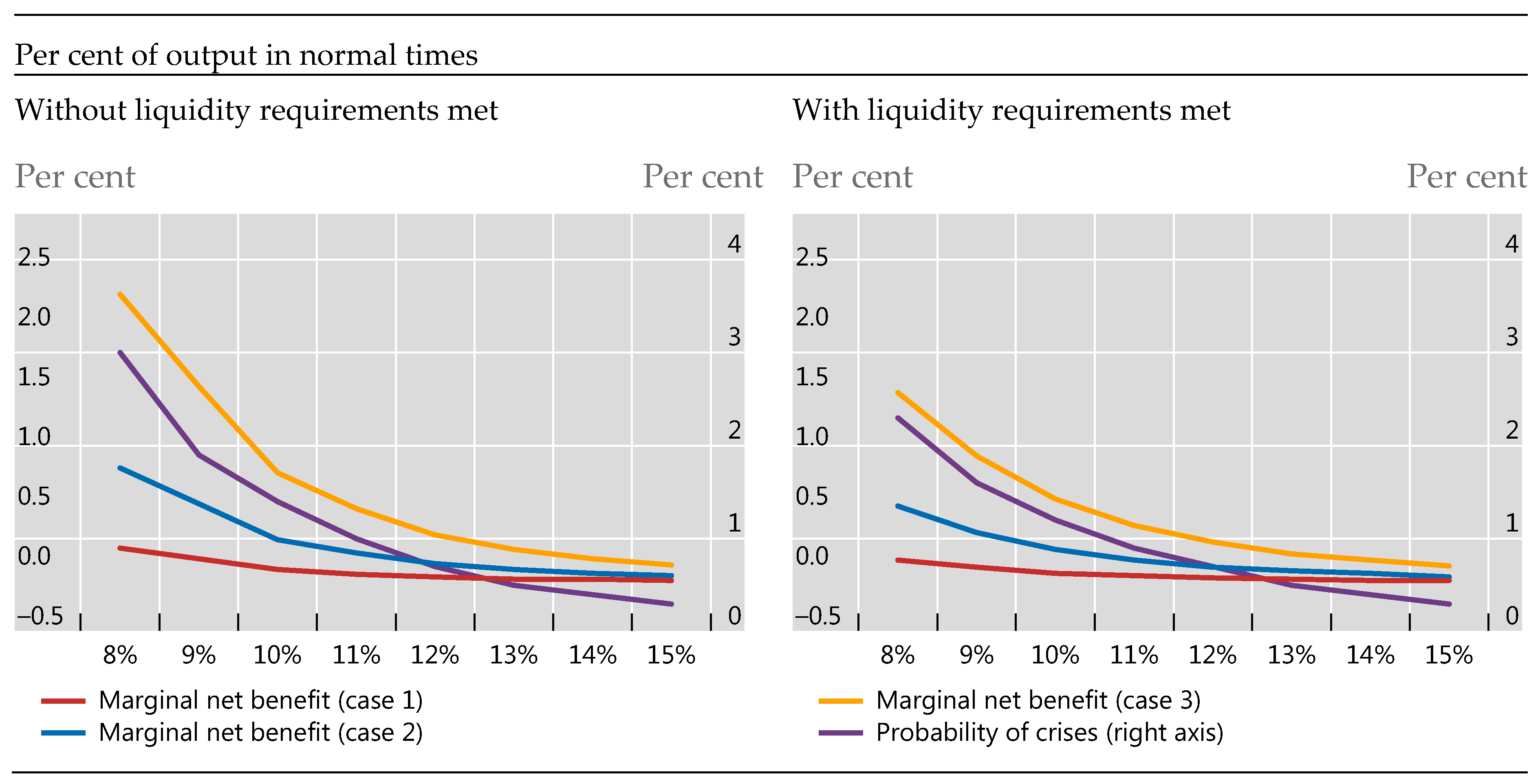
  • The probability of a crisis is 4.6% for a capital ratio of 7% and declines at a diminishing rate to 0.3% for a capital ratio of 15%. Confer BCBS (2010, Table 4): the reduction in the crisis probability from increasing capital hence creates benefits;
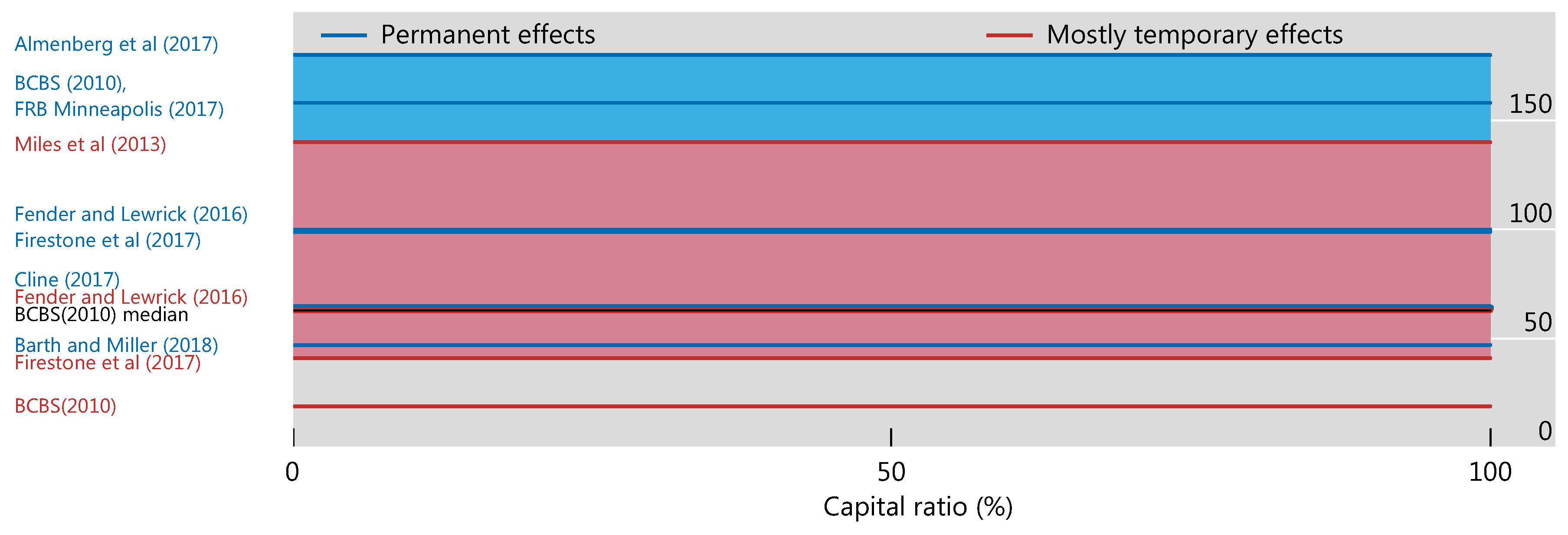
  • The reduction in output in crisis periods relative to normal times is set to three different levels, depending on different assumptions of how a crisis affects trend growth. For the cases of no permanent effects, moderate permanent effects and large permanent effects, the output loss is set to 19%, 63%, and 158% of output in normal times (“normal output”), respectively;
  • The opportunity cost of higher capital resources is estimated to be 0.09% of normal output;
  • The benefit of reducing the amplitude of the business cycle was judged to be too uncertain to be included.
We note that the capital ratio definition applied in BCBS (2010) is tangible common equity (TCE) to risk-weighted assets, whereas some recent studies have focused at common equity Tier 1 (CET1) to risk-weighted assets. In addition, the definition of risk-weighted assets has also changed since the LEI. Fender and Lewrick (2016) suggest using a conversion factor of 0.78, i.e., CET1/RWA = 0.78*TCE/RWA, to transform the calibration used in the LEI to a CET1-basis.
In Figure A1, we replicate the calculations from BCBS (2010) and present the net marginal benefit of higher capital ratios for the three different cost of crises (case 1 = no permanent effects, case 2 = moderate permanent effect, case 3 = large permanent).
The left-hand panel presents the results without liquidity requirements being met. The marginal cost is constant, while the marginal benefit declines with the diminishing effect of capital on the probability of crisis (also depicted in the same plot). The net marginal benefit is bigger when the associated cost of crisis is bigger, but for all cases the net marginal benefit remains positive up to a capital ratio of 10%. The cumulative net benefit—the sum of the net marginal benefits—is positive for all capital ratios considered.
The right-hand panel of Figure A1 presents results that take into account that liquidity requirements are met. This affects the net marginal benefit calculations through the assumption that liquidity requirements lower the probability of crisis as well as the effect of higher capital on that probability.29 As a result, the net marginal benefit schedules are shifted down in the right-hand side panel, but the net marginal benefit remains positive for broadly the same range of capital ratios as in the left-hand side panel.
The implied k* estimates are found where the net marginal benefit turns negative. In the left hand-side panel—without liquidity requirements met—k* is between 10% and 15% TCE/RWA (Basel II), and in the right-hand side panel—with liquidity requirements met—k* is between 9% and 15% TCE/RWA (Basel II).
Figure A1. Net marginal benefits of higher capital ratios in BCBS (2010).
Jrfm 13 00074 g0a1

Appendix B. Benefits and Costs of Capital, Revisited30

Jorda et al. (2017) studied the benefits of bank capitalisation using data on 90 banking crises in 17 OECD countries over the 1870–2013 period. They concluded that while countries with better capitalised banks before a crisis suffer less severe recessions after a crisis, bank capital does not predict the probability of a crisis. Cochrane (2017) subsequently disputed this latter result on the account that the analysis did not treat bank capital as endogenous. This appendix presents results that are based on data from Jorda et al. (2017) and take into consideration Cochrane (2017)’s main methodological concerns by controlling for the past change in the leverage ratio. It also presents new findings on the potential drag from higher capital on bank loan and GDP growth in “normal” times.

Appendix B.1. Benefits of Bank Capital

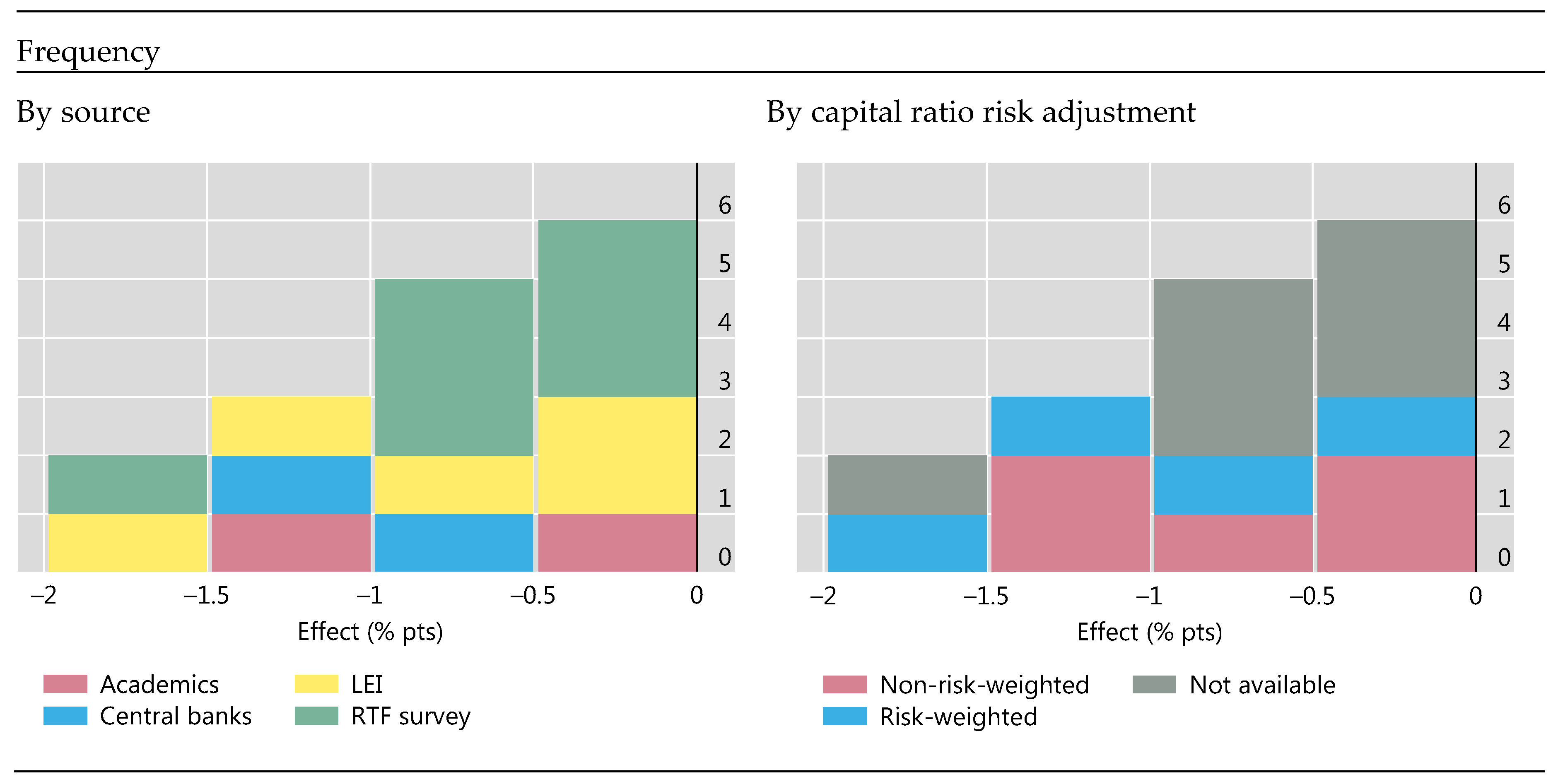
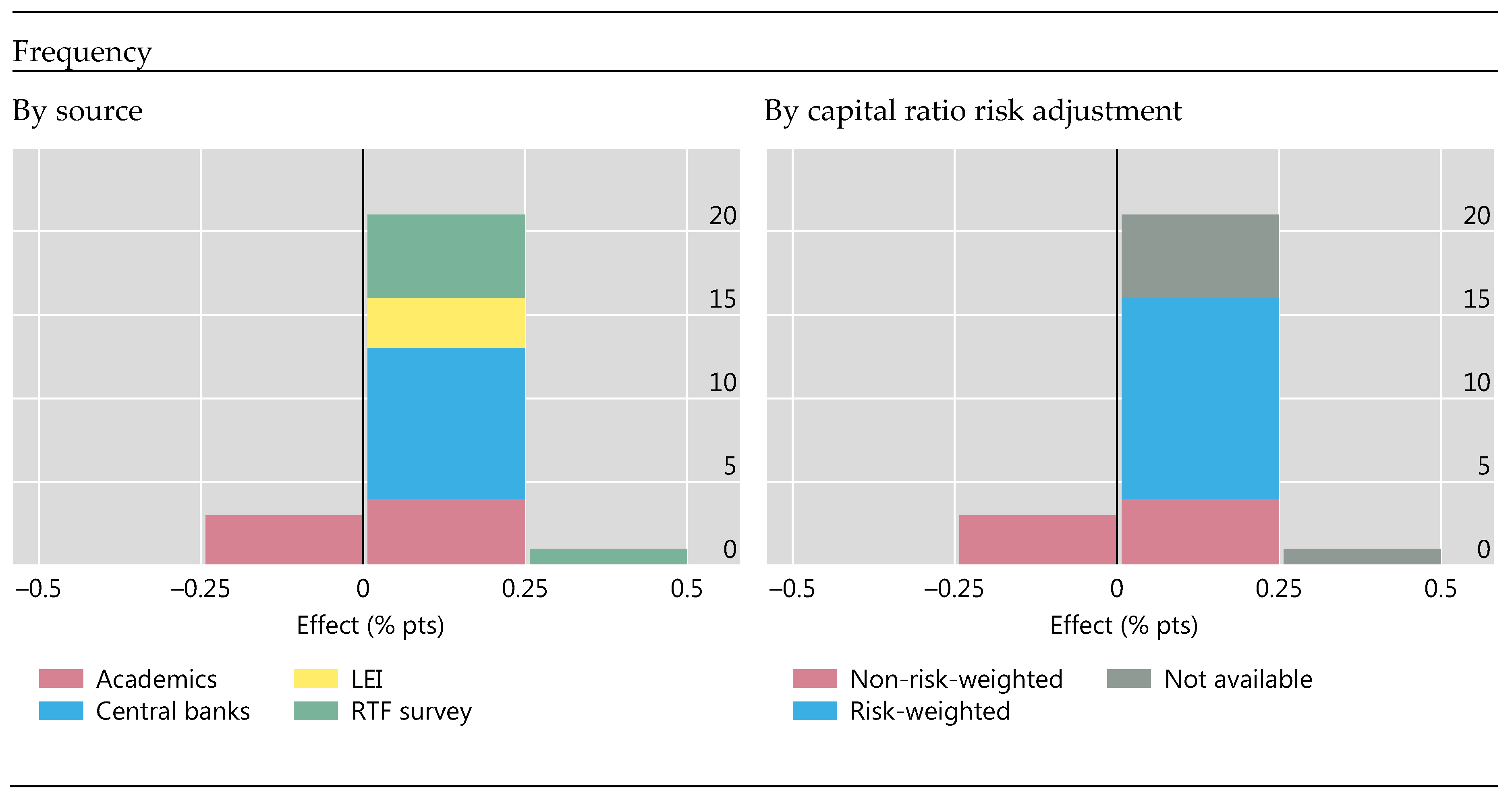
Appendix B.1.1. Lower Probability of a Crisis?
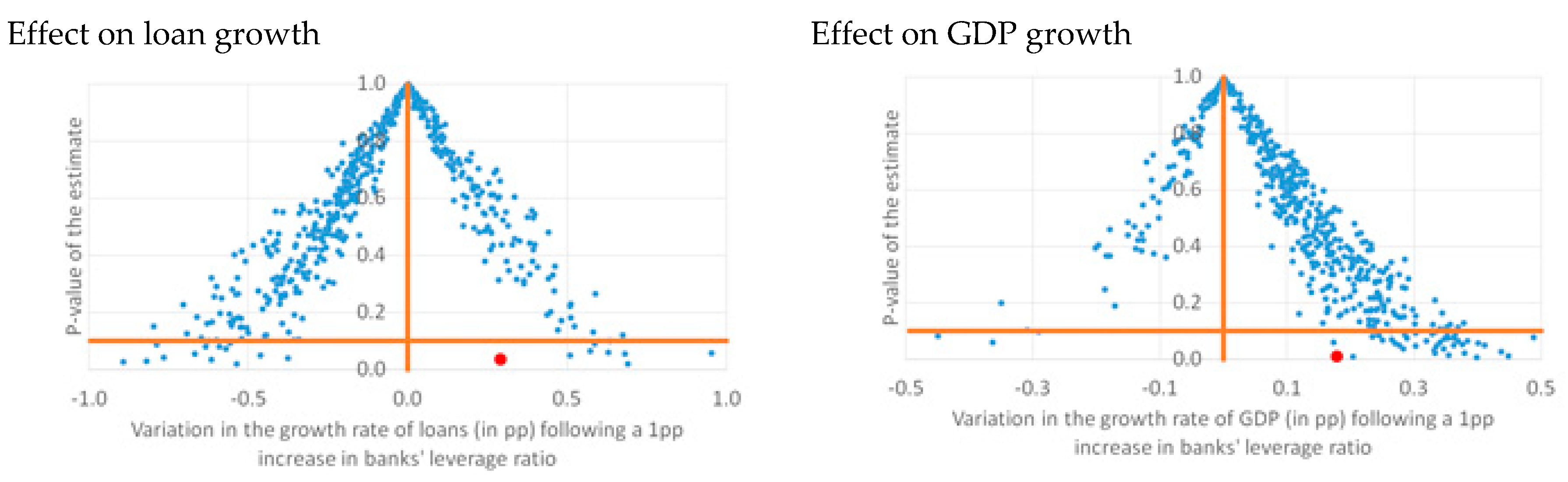
Table A1 reports top down (logit) estimates of the effect of a one percentage point higher leverage ratio (LR) on the probability of a crisis within the next five years. The baseline estimate of the coefficient on the leverage ratio in column (1) is insignificant, suggesting that, historically, crisis risk is not lower when bank leverage is lower. Bank leverage is insignificant even after controlling for change (“build up”) in leverage before the banking crisis (column (2)) and other domestic, financial factors (e.g., house prices, banking sector size) and global factors (year fixed effects). In all cases, the most important predictor of banking crises is bank loan growth.
Table A1. Effect of bank capital on the probability of a banking crisis.
Explanatory Variables(1)(2)(3)(4)
Leverage ratio0.254
(0.577)
0.218
(0.623)
0.778
(0.638)
0.889
(0.448)
Loan growth1.163 **
(0.035)
1.245 ***
(0.009)
1.527 **
(0.033)
1.329 ***
(0.006)
Δ Leverage ratio 5.356
(0.262)
13.586 *
(0.099)
14.557 **
(0.032)
Observations421419242257
ControlsNoNoYesYes
Country FEYesYesYesNo
Year FEYesYesYesYes
Note: Marginal effects. *, **, *** statistically significant at 10%, 5%, 1% thresholds. All explanatory variables are lagged annualised five-year averages. For example, an average 1 percentage point increase in the annual growth rate over five years is associated with a 1.33 percentage point increase in the crisis probability (model (4)).

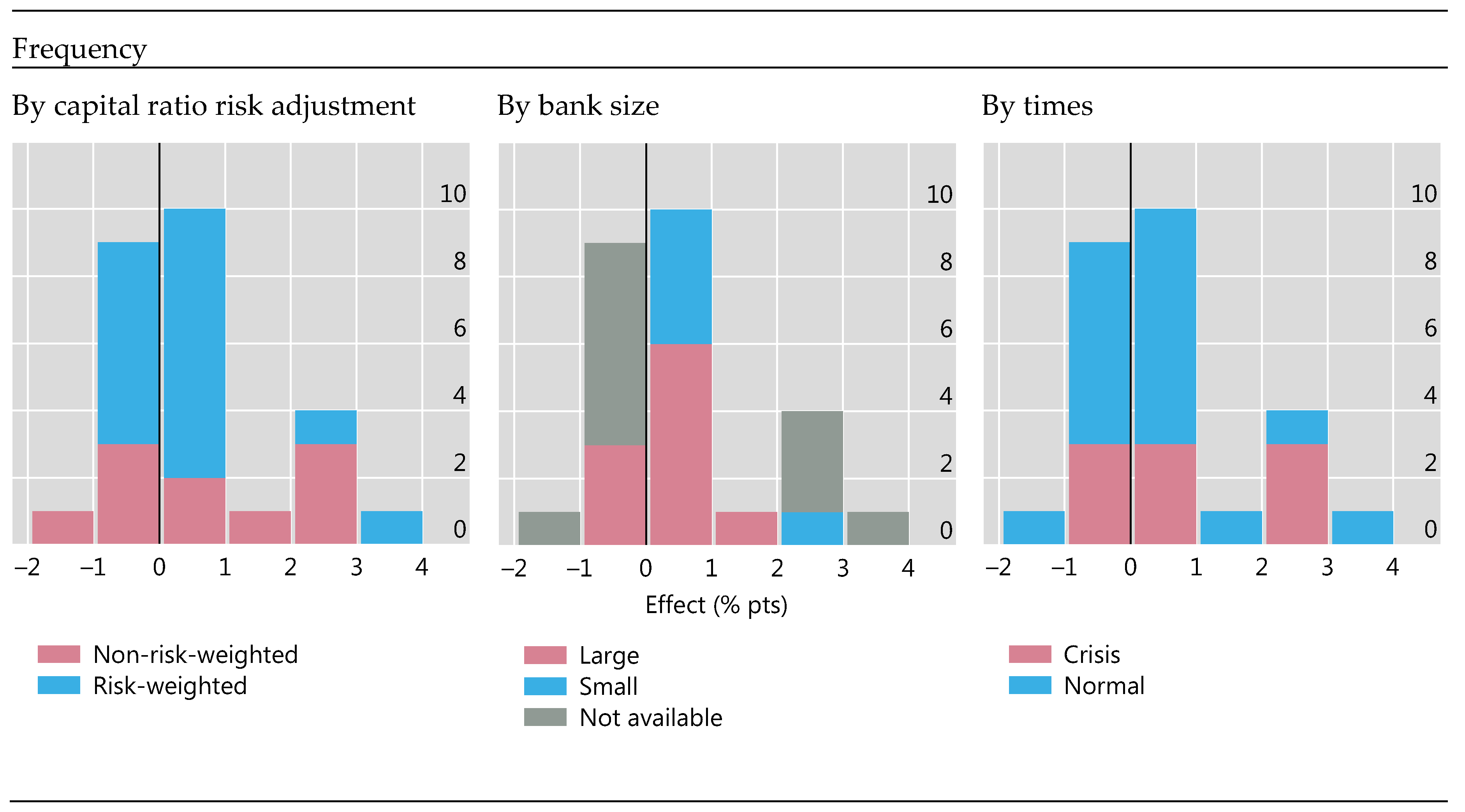
Appendix B.1.2. Lower Crisis Cost?

The two red dots in Figure A2 correspond to the linear regression estimates of the effects of bank capital on bank loan growth (left) and GDP (right) during banking crises. The regression includes multiple control variables similar to model (4) of Table A1 (i.e., house price growth, change in the size of the banking sector, as well as country and time fixed effects). The red dots show that a country whose banks enter a crisis with a one percentage point higher capital ratio experiences 0.29 percentage points higher annual loan and 0.18 percentage points higher GDP growth in the following five years, compared to other countries. The two estimates are both positive and statistically significant. This analysis reinforces the main result of Jorda et al. (2017) that the most important stability benefit of bank capital is to mitigate the cost of crises.
Figure A2. Estimates of the effect of bank capital on loan growth and GDP growth.
Jrfm 13 00074 g0a2

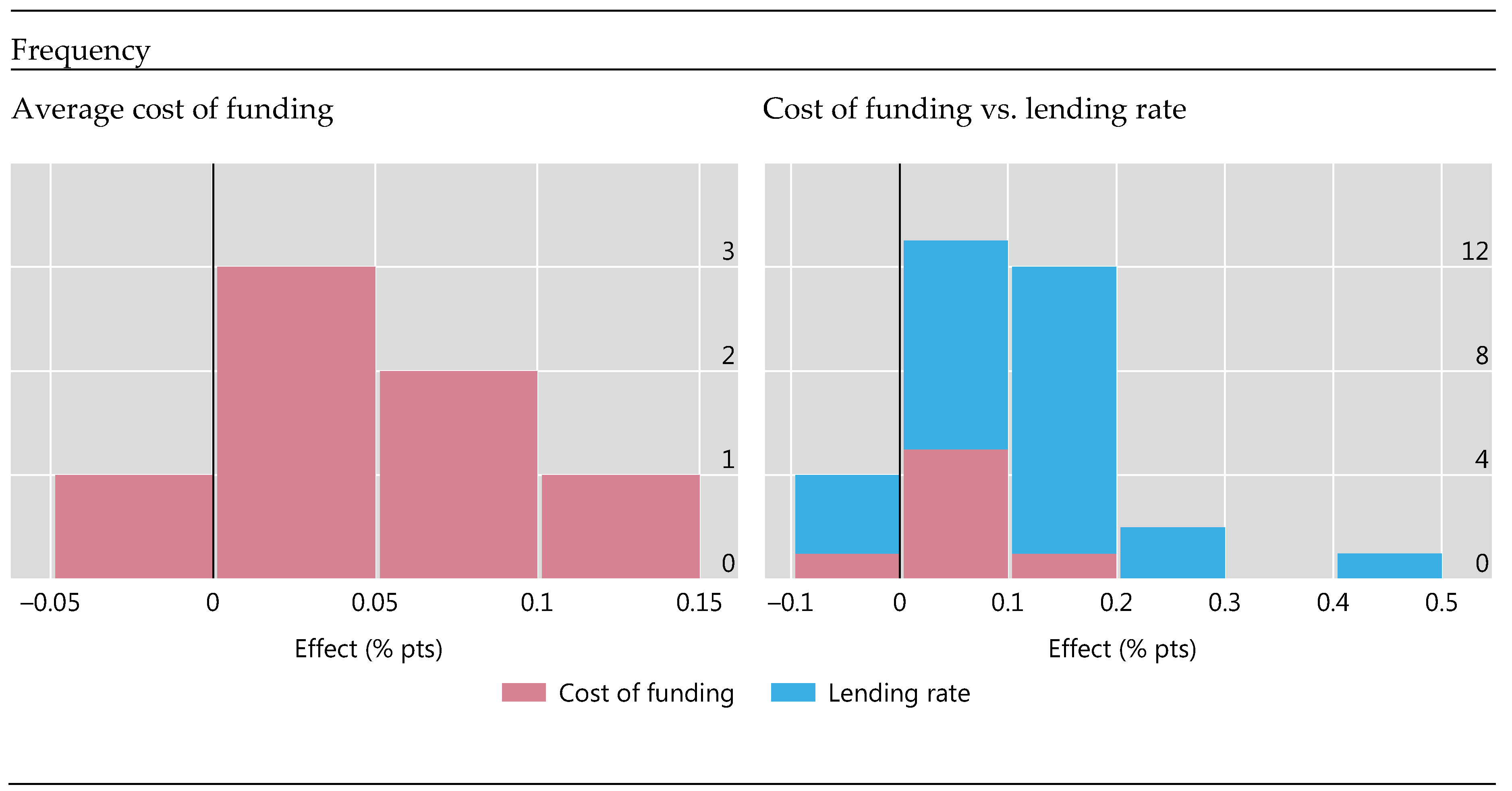
Appendix B.2. Costs of Bank Capital in Normal Times?

The LEI approach assumes that higher required bank capital is a drag on loan growth and thus output in normal (non-crisis) times. Is it? Figure A2 represents the point estimates (x axis) and p-value from regressions of loan growth (left) and GDP growth (right) in “normal times”. To ensure that the estimates are comparable with those for crisis times (see above), 500 samples of “normal time” events are randomly picked among the observations that are at least five years apart from banking crises events in the data. Each blue dot in Figure A2 corresponds to the estimate based on one particular sample of normal times.
Most of the estimates for loan growth (left panel) are negative and non-statistically significant. Only thirteen of the 500 loan growth estimates in the left panel are negative and statistically significant at the 10% threshold, i.e., below the orange, horizontal line. This contrasts with the positive effect during crises (red dot), and emphasises the differential impact of bank capitalisation in normal and crisis times. The right-hand panel shows that most of the estimates for GDP growth are positive but are rarely statistically significant. This suggests that bank capitalisation does not have adverse effects on the real economy in normal times.
In sum, the findings in Jorda et al. (2017) and those here suggest that while higher bank capital may not reduce significantly the probability of a crisis, it does significantly lower the cost of a crisis by sustaining bank lending during the resulting recession. In addition, in normal times, bank capital does not seem to be negatively correlated with loan growth or GDP growth.

Appendix C. Competition and Regulatory Reform Interactions

The LEI and later studies did not consider how competition among banks and from non-bank lenders might affect k*. Competition matters as it is a key determinant of banks’ ability to pass on higher funding costs to borrowers and the resulting drag on economic activity, and competition may directly affect financial stability.
In more competitive markets, banks’ narrower margins offer less scope to absorb regulatory costs imposed across the sector. In less competitive markets, banks with market power can absorb (at least partly) regulatory costs through lower profits. In fact, full pass-through would not be profit maximising for a firm with market power.31
Banks also compete head-to-head for borrowers with non-bank intermediaries (insurance and finance companies, peer-to-peer lenders, etc.) and directly with bond markets for large corporate borrowers. More intense competition from these non-bank lenders means lower pass-through of bank costs to loan rates and a smaller resulting drag on output.32
Competition can have differential impacts across sectors and economies with different financial structures. Small and medium-sized enterprises (SME) may find access to bond markets limited and are ‘captured’ by the banks. Banks may be able to pass costs through to SME lending to a greater extent than for large corporates, who have better access to bond markets. Likewise, banks operating in more “bank-centric” economies with fewer non-bank funding sources may have greater ability to pass through costs. All else the same, the drag from higher capital requirements or other reforms in more bank-centric economies will be higher.
Just as differences in the degree of competition may influence optimal capital, regulatory reforms may also affect competition. For example, the implicit subsidy for too-big-to-fail (TBTF) banks reduced their funding costs and provided a competitive advantage vis-à-vis smaller banks. Reforms that reduce that funding advantage can heighten competition faced by TBTF banks. That said, competition may be diminished where the costs of regulatory reforms fall disproportionately on smaller banks or banks facing higher external funding costs.
Overall, the influence of competition on optimal capital ratios, though difficult to assess, bears consideration.33 Ignoring it, as the LEI and later studies have, adds to the uncertainty surrounding the estimates and may present a margin for improvement.

Appendix D. Relation between Marginal Benefits and Optimal Levels of Capital

Figure A3 illustrates that a comparison of the marginal benefits at given capital levels is not directly informative for assessing optimal capital levels, as the transitive properties depend on the shape of the marginal benefit curves. The figure compares the marginal benefits under three different models of crisis probabilities A, B, and C. For simplicity, the marginal cost is assumed to be constant.
For capital levels between k1 and k2, the marginal benefits in model C exceed the marginal benefits in model B, which in turn exceed the marginal benefits in model A. Thus, for this range of capital levels, MBC > MBB > MBA. However, while the optimal level of capital is also the highest for model C, the optimal level of capital for model A exceeds the optimal capital level for model B, thus k*C > k*A > k*B. This reflects the steeper marginal benefits curve in model B compared to model A.
Hence, the relative order of the marginal benefits at given levels of capital (in this case, between k1 and k2) does not directly map into an identical relative order of optimal capital levels.
Figure A3. Marginal costs, marginal benefits and optimal levels of capital.
Jrfm 13 00074 g0a3

References

  1. Admati, Anat R., Peter M. DeMarzo, Martin Hellwig, and Paul Pfleiderer. 2013. Fallacies, Irrelevant Facts, and Myths in the Discussion of Capital Regulation: Why Bank Equity Is Not Expensive. Working Paper No. 2065. Stanford: Stanford Business School. [Google Scholar]
  2. Aikman, David, Andrew G. Haldane, Marc Hinterschweiger, and Sujit Kapadia. 2018. Rethinking Financial Stability. Working Paper 712. London: Bank of England. [Google Scholar]
  3. Aiyar, Shekhar, Charles W. Calomiris, John Hooley, Yevgeniya Korniyenko, and Tomasz Wieladek. 2014a. The International Transmission of Bank Capital Requirements: Evidence from the UK. Journal of Financial Economics 113: 368–82. [Google Scholar] [CrossRef]
  4. Aiyar, Shekhar, Charles W. Calomiris, and Tomasz Wieladek. 2014b. Does Macro-Prudential Regulation Leak? Evidence from a UK Policy Experiment. Journal of Money, Credit and Banking 46: 181–214. [Google Scholar] [CrossRef]
  5. Aiyar, Shekhar, Charles W. Calomiris, and Tomasz Wieladek. 2016. How Does Credit Supply Respond to Monetary Policy and Bank Minimum Capital Requirements? European Economic Review 82: 142–65. [Google Scholar] [CrossRef]
  6. Almenberg, Johan, Markus Andersson, Daniel Buncic, Cristina Cella, Paolo Giordani, Anna Grodecka, Kasper Roszbach, and Gabriel Söderberg. 2017. Appropriate Capital Ratios in Major Swedish Banks—New Perspectives. Stockholm: Sveriges Riksbank, Available online: http://archive.riksbank.se/Documents/Rapporter/Staff%20memo/Staff_memo_170519_eng.pdf (accessed on 1 May 2019).
  7. Baker, Malcolm P., and Jeffrey Wurgler. 2013. Would Stricter Capital Requirements Raise the Cost of Capital? Bank Capital Regulation and the Low Risk Anomaly. Working Paper. New York: New York University Stern Business School, Available online: http://people.stern.nyu.edu/jwurgler/papers/Bank%20Capital%20Regulation.pdf (accessed on 1 May 2019).
  8. Barrell, Ray, E. Philip Davis, Tatiana Fic, Dawn Holland, Simon Kirby, and Iana Liadze. 2009. Optimal Regulation of Bank Capital and Liquidity: How to Calibrate New International Standards. London: Bank of England. [Google Scholar]
  9. Barth, James R., and Stephen Matteo Miller. 2018. Benefits and Costs of a Higher Bank Leverage Ratio. Journal of Financial Stability 38: 37–52. [Google Scholar] [CrossRef]
  10. Basel Committee on Banking Supervision (BCBS). 2010. An Assessment of the Long-Term Economic Impact of Stronger Capital and Liquidity Requirements. Available online: http://www.bis.org/publ/bcbs173.htm (accessed on 1 May 2019).
  11. Behn, Markus, Rainer Haselmann, and Paul Wachtel. 2016. Procyclical Capital Regulation and Lending. The Journal of Finance 71: 919–56. [Google Scholar] [CrossRef]
  12. Benetton, Matteo, Peter Eckley, Nicola Garbarino, Liam Kirwin, and Georgia Latsi. 2017. Specialisation in Mortgage Risk under Basel II. Bank of England Working Paper no 639. Available online: https://papers.ssrn.com/sol3/papers.cfm?abstract_id=2900165 (accessed on 1 May 2019).
  13. Bernanke, Ben S., Cara S. Lown, and Benjamin M. Friedman. 1991. The Credit Crunch. Brookings Paper on Economic Activity, 205–39. [Google Scholar] [CrossRef] [Green Version]
  14. Berrospide, Jose M., and Rochelle M. Edge. 2010. The Effects of Bank Capital on Lending: What Do We Know, and What Does It Mean? International Journal of Central Banking 6: 5–54. [Google Scholar]
  15. Bank for International Settlements (BIS). 2015. Assessing the Economic Costs and Benefits of TLAC Implementation. Available online: http://www.bis.org/publ/othp24.pdf (accessed on 1 May 2019).
  16. Bordo, Michael, Barry Eichengreen, Daniela Klingebiel, and Maria Soledad Martinez-Peria. 2001. Financial Crisis-Lessons from the Last 120 Years. Economic Policy 16: 51–82. [Google Scholar]
  17. Bridges, Jonathan, David Gregory, Mette Nielsen, Silvia Pezzini, Amar Radia, and Marco Spaltro. 2014. The Impact of Capital Requirements on Bank Lending. Bank of England Working Paper no 486. Available online: http://papers.ssrn.com/sol3/papers.cfm?abstract_id=2388773 (accessed on 1 May 2019).
  18. Brooke, Martin, Oliver Bush, Robert Edwards, Jas Ellis, Bill Francis, Rashmi Harimohan, Katharine Neiss, and Caspar Siegert. 2015. Measuring the Macroeconomic Costs and Benefits of Higher UK Bank Capital Requirements. Bank of England Financial Stability Paper no 35. Available online: http://www.bankofengland.co.uk/-/media/boe/files/financial-stability-paper/2015/measuring-the-macroeconomic-costs-and-benefits-of (accessed on 1 May 2019).
  19. Cline, William R. 2017. The Right Balance for Banks: Theory and Evidence on Optimal Capital Requirements. New York: Columbia University Press. [Google Scholar]
  20. Cochrane, John. 2017. Capital Cause and Effect. Blog. Available online: http://johnhcochrane.blogspot.com/2017/04/capital-cause-and-effect.html (accessed on 1 May 2019).
  21. Cosimano, Thomas F., and Dalia Hakura. 2011. Bank Behavior in Response to Basel III: A Cross-Country Analysis. International Monetary Fund Working Paper 11/119. Available online: http://www.imf.org/external/pubs/ft/wp/2011/wp11119.pdf (accessed on 1 May 2019).
  22. Covas, Francisco, and John C. Driscoll. 2014. Bank Liquidity and Capital Regulation in General Equilibrium. Federal Reserve Board Finance Economics Discussion Series Working Paper No 2014–85. Washington: Federal Reserve Board. [Google Scholar]
  23. Dagher, Jihad, Giovanni Dell’Arriccia, Luc Laeven, Lev Ratnovski, and Hui Tong. 2016. Benefits and Costs of Bank Capital, International Monetary Fund Staff Discussion Note 16/04. Available online: http://www.imf.org/external/pubs/ft/sdn/2016/sdn1604.pdf (accessed on 1 May 2019).
  24. de-Ramon, Sebastián, Zanna Iscenko, Matthew Osborne, Michael Straughan, and Peter Andrews. 2012. Measuring the Impact of Prudential Policy on the Macroeconomy: A Practical Application to Basel III and Other Responses to the Financial Crisis. Financial Services Authority Occasional Paper, No 42. London: Financial Services Authority. [Google Scholar]
  25. Dell’Arriccia, Giovanni, Luc Laeven, and Gustavo A. Suarez. 2017. Bank Leverage and Monetary Policy’s Risk-Taking Channel: Evidence from the United States. The Journal of Finance 72: 613–54. [Google Scholar] [CrossRef]
  26. Dewatripont, Mathias, Diana Hancock, Emrah Arbak, Janet Mitchell, Josef Schroth, Olivier de Bandt, Claire Labonne, Monika Bucher, Daniel Foos, Roberta Fiori, and et al. 2016. Literature Review on Integration of Regulatory Capital and Liquidity Instruments. Working Papers. Basel: Basel Committee on Banking Supervision. [Google Scholar]
  27. Federal Reserve Bank of Minneapolis. 2017. The Minneapolis Plan to End Too Big to Fail. Available online: http://www.minneapolisfed.org/~/media/files/publications/studies/endingtbtf/the-minneapolis-plan/the-minneapolis-plan-to-end-too-big-to-fail-final.pdf?la=en (accessed on 1 May 2019).
  28. Fender, Ingo, and Ulf Lewrick. 2016. Adding It All Up: The Macroeconomic Impact of Basel III and Outstanding Reform Issues. Working Paper no 591. Basel: Bank for International Settlements, Available online: http://www.bis.org/publ/work591.pdf (accessed on 1 May 2019).
  29. Firestone, Simon, Amy Lorenc, and Benjamin Ranish. 2017. An Empirical Economic Assessment of the Costs and Benefits of Bank Capital in the US. Federal Reserve Board Finance and Economics Discussion Series Working Paper 2017-34. Washington, DC: Federal Reserve Board Finance and Economics. [Google Scholar]
  30. Furceri, Davide, and Annabelle Mourougane. 2012. The Effect of Financial Crises on Potential Output from OECD Countries. Journal of Macroeconomics 34: 822–32. [Google Scholar] [CrossRef]
  31. Gambacorta, Leonardo, and Hyun Song Shin. 2018. Why Bank Capital Matters for Monetary Policy. Journal of Financial Intermediation 25: 17–29. [Google Scholar] [CrossRef] [Green Version]
  32. Glancy, David, and Robert J. Kurtzman. 2018. How do Capital Requirements Affect Loan Rates? Evidence from High Volatility Commercial Real Estate. Board of Governors of the Federal Reserve System. Available online: http://papers.ssrn.com/sol3/papers.cfm?abstract_id=3202509 (accessed on 1 May 2019).
  33. Homar, Timotej, and Sweder J. G. van Wijnbergen. 2017. Bank Recapitalization and Economic Recovery after Financial Crises. Journal of Financial Intermediation 32: 16–28. [Google Scholar] [CrossRef]
  34. International Monetary Fund. 2018. The Global Recovery 10 Years after the 2008 Financial Meltdown. In World Economic Outlook. Washington, DC: International Monetary Fund, chp. 2. pp. 71–100. [Google Scholar]
  35. Iyer, Rajkamal, José-Luis Peydró, Samuel da-Rocha-Lopes, and Antoinette Schoar. 2014. Interbank Liquidity Crunch and the Firm Credit Crunch: Evidence from the 2007–2009 Crisis. The Review of Financial Studies 27: 347–72. [Google Scholar] [CrossRef]
  36. Jorda, Oscar, Björn Richter, Moritz Schularick, and Alan M. Taylor. 2017. Bank Capital Redux: Solvency, Liquidity, and Crisis. NBER Working Paper No 23287. Cambridge: NBER. [Google Scholar]
  37. Junge, Georg, and Peter Kugler. 2013. Quantifying the Impact of Higher Capital Requirements on the Swiss Economy. Swiss Journal of Economics and Statistics 149: 313–56. [Google Scholar] [CrossRef] [Green Version]
  38. Kapan, Tümer, and Camelia Minoiu. 2018. Balance Sheet Strength and Bank Lending: Evidence from the Global Financial Crisis. Journal of Banking and Finance 92: 35–50. [Google Scholar] [CrossRef]
  39. Kashyap, Anil K., Jeremy C. Stein, and Samuel Hanson. 2010. An Analysis of the Impact of “Substantially Heightened” Capital Requirements on Large Financial Institutions. Available online: http://faculty.chicagobooth.edu/anil.kashyap/research/papers/an_analysis_of_the_impactof_substantially_heightened-Capital-Requirements-on-Financial-Institutions.pdf (accessed on 1 May 2019).
  40. Kim, Dohan, and Wook Sohn. 2017. The Effect of Bank Capital on Lending: Does Liquidity Matter? Journal of Banking and Finance 77: 95–107. [Google Scholar] [CrossRef]
  41. Valencia, Fabian, and Mr Luc Laeven. 2008. Systemic Banking Crises: A New Database. Working Paper no. WP/08/224. International Monetary Fund: Available online: http://www.imf.org/external/pubs/ft/wp/2008/wp08224.pdf (accessed on 1 May 2019).
  42. Laeven, Luc, and Fabian Valencia. 2012. Systemic Banking Crises Database: An Update. International Monetary Fund Working Paper no. WP/12/163. Available online: http://www.imf.org/external/pubs/ft/wp/2012/wp12163.pdf (accessed on 1 May 2019).
  43. Locarno, Alberto. 2011. The Macroeconomic Impact of Basel III on the Italian Economy. Banca d’Italia Working Papers no 88. Rome: Banca d’Italia. [Google Scholar]
  44. Martinez-Miera, David, and Rafael Repullo. 2010. Does Competition Reduce the Risk of Bank Failure? Review of Financial Studies 23: 3638–64. [Google Scholar] [CrossRef] [Green Version]
  45. Mayes, David G., and Hanno Stremmel. 2014. The Effectiveness of Capital Adequacy Measures in Predicting Bank Distress. Vienna: SUERF Studies, no. 2014/1. [Google Scholar]
  46. Mikkelsen, Jakob Guldbæk, and Jesper Pedersen. 2017. A Cost-Benefit Analysis of Capital Requirements for the Danish Economy. Working Paper no 123. Copenhagen: Danmarks National Bank. [Google Scholar]
  47. Miles, David, Jing Yang, and Gilberto Marcheggiano. 2013. Optimal Bank Capital. Economic Journal 123: 1–37. [Google Scholar] [CrossRef]
  48. Reinhart, Carmen M., and Kenneth S. Rogoff. 2008. This Time Is Different: A Panoramic View of Eight Centuries of Financial Crisis. NBER Working Paper 13882. Cambridge: NBER. [Google Scholar]
  49. Romer, Christina D., and David H. Romer. 2017a. New Evidence on the Impact of Financial Crises in Advanced Countries. American Economic Review 107: 3072–118. [Google Scholar] [CrossRef] [Green Version]
  50. Romer, Christina D., and David H. Romer. 2017b. Why Some Times are Different: Macroeconomic Policy and the Aftermath of Financial Crises. Economica 85: 1–40. [Google Scholar] [CrossRef]
  51. Roulet, Caroline. 2018. Basel III: Effects of Capital and Liquidity Regulations on European Bank Lending. Journal of Economics and Business 95: 26–46. [Google Scholar] [CrossRef]
  52. Santos, Joao A. C., and Andrew Winton. 2013. Bank Capital, Borrower Power, and Loan Rates. Available online: http://papers.ssrn.com/sol3/papers.cfm?abstract_id=1343897 (accessed on 1 May 2019).
  53. Slovik, Patrick, and Boris Cournède. 2011. Macroeconomic Impact of Basel III. Organisation for Economic Co-Operation and Development Economics Department Working Papers no 884. Available online: http://www.oecd.org/officialdocuments/publicdisplaydocumentpdf/?cote=ECO/WKP (accessed on 1 May 2019).
  54. Sutorova, Barbora, and Petr Teplý. 2013. The Impact of Basel III on Lending Rates of EU Banks. Czech Journal of Economics and Finance 63: 226–43. [Google Scholar]
  55. Sveriges Riksbank. 2011. Appropriate Capital Ratios in Major Swedish Banks. Available online: http://archive.riksbank.se/Upload/Rapporter/2011/rap_appropriate_capital_ratio_in_major_swedish_banks_111206_eng.pdf (accessed on 1 May 2019).
  56. Varian, Hal R. 1992. Microeconomic Analysis. Rockville: W. W. Norton & Company. [Google Scholar]
  57. Vickers, John. 2016. The Systemic Risk Buffer for UK Banks: A Response to the Bank of England’s Consultation Paper. Journal of Financial Regulation 2: 264–82. [Google Scholar] [CrossRef]
  58. Zigraiova, Diana, and Tomas Havranek. 2016. Bank Competition and Financial Stability: Much Ado About Nothing? Journal of Economic Surveys 30: 944–81. [Google Scholar] [CrossRef] [Green Version]
1
In the original LEI as well as in later studies the analysis refers to capital held, so that it does not distinguish between the minimum capital requirement and additional capital that banks may hold in excess of the minimum requirement. See Dewatripont et al. (2016) for a discussion of the costs and benefits of bank capital requirements outside of this stabiliser/drag framework.
2
Miles et al. (2013) and Barth and Miller (2018) are the only papers published thus far in economics journals. Cline (2017) is a book published by the Peterson Institute. A working paper version is available at piie.com/system/files/documents/wp16-6.pdf. Barrell et al. (2009) is a notable precursor to the LEI. See also de Ramon et al. (2012).
3
To be able to compare BCBS (2010) with a given later study, k*—defined as TCE/Basel II RWA—should be converted to the capital measure used in that later study. The conversion of the BCBS (2010) estimate is specific to the country and time-period of interest. For example, Firestone et al. (2017) provide a conversion estimate of the BCBS optimal capital range—10–15% in TCE/RWA (Basel II)—to 9.3–15.5% in Tier 1/RWA (Basel III) space by using a cross-section of US banks. Brooke et al. (2015) provide a conversion estimate of the BCBS (2010) optimal capital number for the UK—assuming moderate permanent effects of crises, they estimate a range of 16–19% in Tier 1/RWA (Basel III) space using samples of Euro-area banks and UK banks.
4
The LEI study concludes that the unconditional, annual probability of a banking crisis over the 1985–2009 period for G10 countries is at 4–5%, based on Reinhart and Rogoff (2008) and Laeven and Valencia (2008) crisis dating. Cline (2017, p. 28) notes that over the 1977–2015 period the probability is 2.6%.
5
Rapid credit growth (high credit/GDP) is invariably a highly significant, positive predictor of crisis in top down models. That is notable, if not surprising, because slower credit growth is considered a cost or drag from higher capital requirements, i.e., credit growth enters both sides of the costs and benefit calculation.
6
This contrasts with an extensive literature that finds capital ratios are predictive of bank failure. See for example Mayes and Stremmel (2014).
7
Bordo et al. (2001) estimated that the cumulative costs of a crisis in the post-Bretton Woods era was 7% of GDP, but that assumes no permanent effects. Reinhart and Rogoff (2008) found the average peak-to-trough decline in GDP, which also assumes only temporary effects, following a financial crisis is 9.3%.
8
The interventions (suspended convertibility, recapitalisation, nationalisation, liquidity support, guarantees, or asset purchases) must also be sufficiently large to qualify as a crisis indicator: liquidity support of at least 5% of deposits and liabilities to non-residents, restructuring costs of at least 3% of GDP, asset purchases of at least 5% of GDP, significant bank nationalisations or bank guarantees.
9
The narrative approach involves a mix of judgment and rules. For example, a ‘minor crisis’ is identified by three characteristics: (1) OECD perception of significant financial sector problems; (2) a belief that the problems are significantly affecting aggregate credit supply or growth; and (3) a belief the problems are not so severe as to be central to recent macroeconomic events or current expectations.
10
The smaller, GLS (generalised least squares) estimate in the right panel may better apply to advanced economies as it down-weights smaller/less stable emerging economies.
11
Both stages use data from OECD countries from 1960 to 2008.
12
They assume a 2.7% discount rate. They use the GLS results from Romer and Romer (2017a) as GLS weights the larger, less volatile economies more and is thus more relevant for the United States.
13
Brooke et al. (2015) also adapt the Romer and Romer method, extending their sample in time and eliminating countries that they judged were less relevant to the UK. They also make adjustments based on the expected effect of TLAC and other structural changes to the banking system. Like Romer and Romer, Brooke et al. (2015) examine the marginal impact of a financial crisis, i.e., the effect over and above the general recession element that would have occurred anyway. Separating the marginal additional cost of a financial crisis leads to a considerably lower estimate of the cost of a crisis and, therefore, a lower estimate for k*. Some studies have simply used the 2010 LEI estimates, relied on previous work, or used relatively simple assumptions to calibrate the cost of a crisis. The Federal Reserve Bank of Minneapolis (2017) used the high end of the BCBS (2010) range. Miles et al. (2013) assume that GDP falls by 10% the first year, 7.5% the next five years, and then 2.5% forever. Cline (2017) uses a parameterisation, distinguished by assumptions about forgone investment in capital and that capital’s depreciation. Barth and Miller (2018) roughly follow Miles et al. (2013). BIS (2015) uses two calibrations as alternatives: Cline (2017) and the original BCBS (2010) median. Almenberg et al. (2017) use an estimate of the cost of prior Swedish crises, acknowledging the great uncertainty around this estimate.
14
Brooke et al. (2015) and Firestone et al. (2017) both incorporate this study in their analysis. BIS (2015) finds that TLAC and enhanced resolution planning reduce crisis probability and/or costs.
15
In addition, Brooke et al. (2015) find that crises would be around 25% more likely to happen absent effective resolution regimes, drawing on empirical studies which suggest that banks which expect to be bailed out are not therefore subject to market discipline and take more risk, raising the chance that a major bank will fail by around 30%.
16
If the higher cost of equity to banks reflects only the tax advantage of debt (and no other frictions), it is arguable whether the drag from higher required capital represents a social cost.
17
Almenberg et al. (2017) draw on the literature that estimates the effect of higher capital or capital requirements on lending spreads and does not estimate the MM offset directly. Fender and Lewrick (2016) use the same cost of capital and lending spread assumptions as those used in the LEI while acknowledging that they were likely highly conservative based on more recent work and revised the definition of capital. As a consequence, they use the LEI corrected by the conversion factor CET1/RWA = 0.78 TCE/RWA, hence the impact of 9 bps * (1/0.78) = 12 bps on GDP of a 1 percentage point increase in CET1/RWA.
18
Table 2 in Almenberg et al. (2017) summarises recent estimates in seven studies of MM offset (including four not considered here) showing an estimated range between 41 and 100%.
19
If the cost of meeting the higher liquidity requirements (from the NSFR) is considered, the estimated median impact implies an additional 0.08% loss in steady state GDP, independently of the level of capital.
20
All units in this paragraph are per a one percent increase in the leverage ratio, while those in Table 1 are measured with respect to the risk-weighted ratio. Miles et al. (2013) conclude that a Tier 1 increase that would halve leverage would reduce equilibrium output by 0.15%. In their exercise, leverage—computed as assets/Tier 1 capital—falls from 30 to 15, which in Basel III terms would be a leverage ratio increasing from 3.3% to 6.6%. Assuming that leverage ratios increase as capital requirements increase and linearity, each percentage point increase in the leverage ratio would reduce equilibrium GDP by approximately one third (0.045%) of their estimate.
21
Other, more recent, LEI studies (see Section 2) are less conservative, assuming that the cost of equity is lower for better capitalised banks, and they therefore find a lower effect of bank capitalisation on banks’ overall cost of funding.
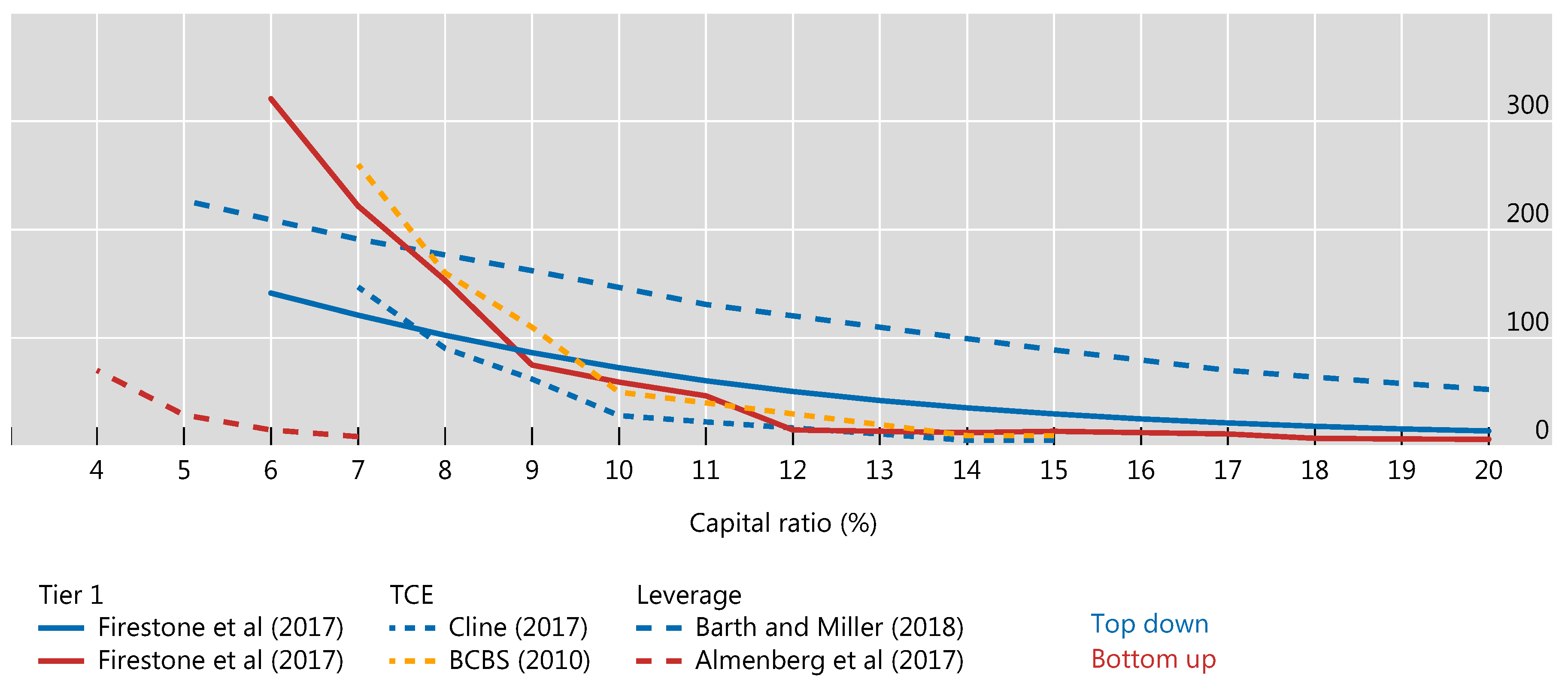
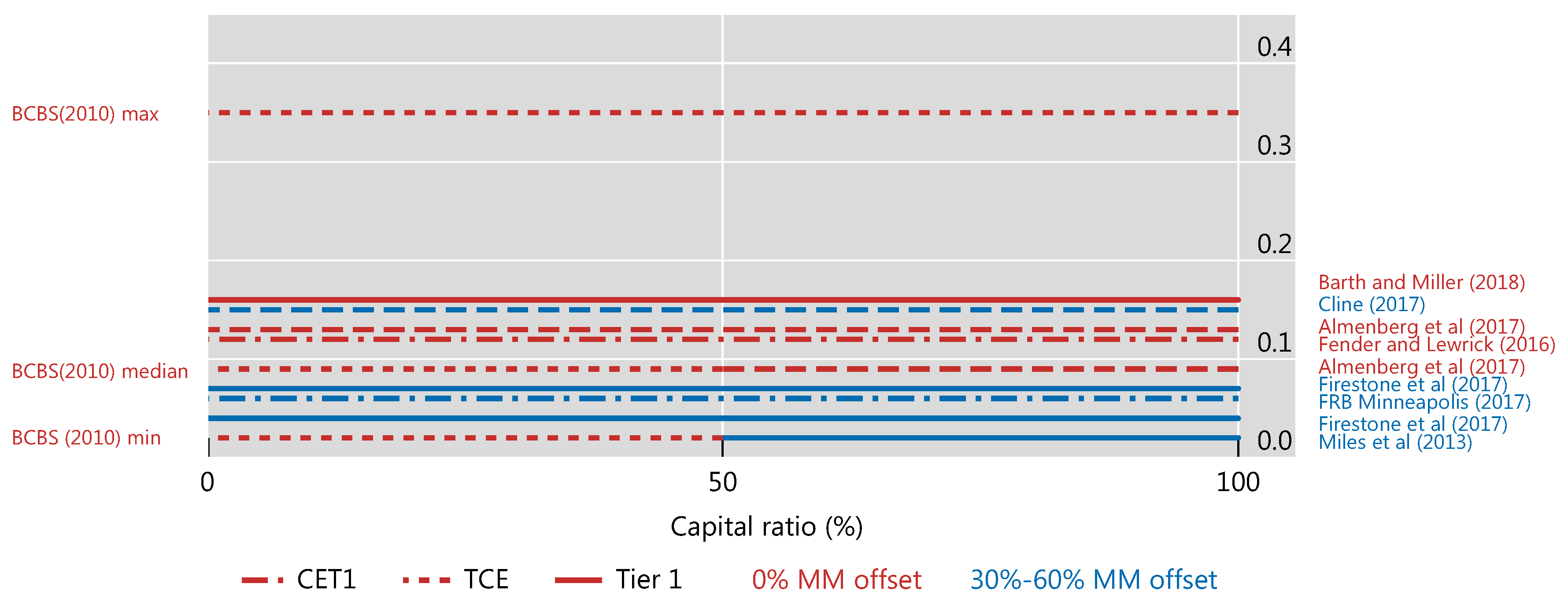
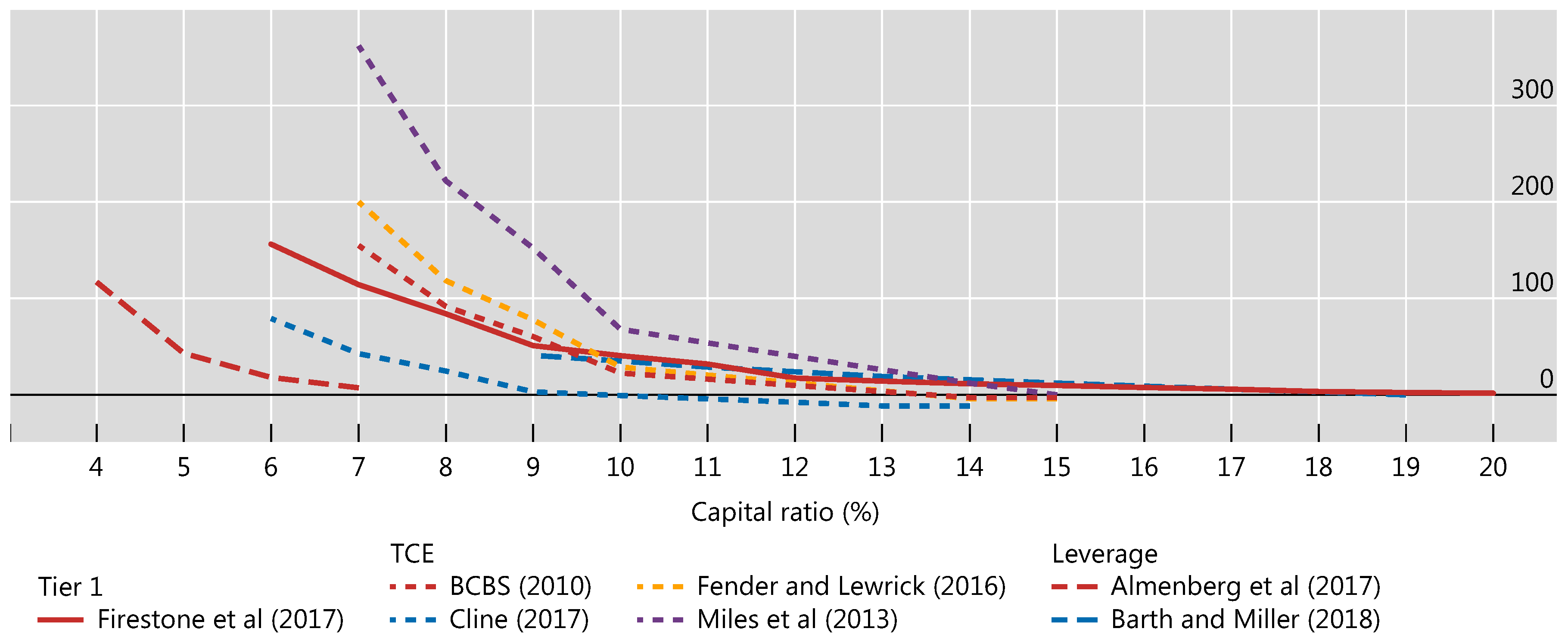
22
In some cases, estimates are approximate because values were derived from figures provided in the study. The full range of studies covered in Section 2 could not be included in these charts due to insufficient data availability in the respective studies.
23
The marginal cost and marginal benefit estimates derived from Table 1 would be for the respective initial levels of capital in each study. They cannot be used to infer optimal capital levels as discussed in Appendix D.
24
Increases in loan spreads owing to capital increases used in subsequent LEI studies tended to be lower than the 13 basis points reported in LEI (Table 1). The mean of 12 basis points for this marginal effect in the piecemeal studies confirms the LEI estimate. (This is the average of standardised estimates reported in FRAME for Benetton et al. (2017), Cosimano and Hakura (2011), Dagher et al. (2016), Glancy and Kurtzman (2018), Santos and Winton (2013), Slovik and Cournede (2011), and Sutorova and Teply (2013)). We focus on marginal costs here rather than on its components because some studies use macroeconomic models that do not consider loan spreads.
25
Piecemeal studies (see FRAME standardised estimates for Covas and Driscoll (2014) and Locarno (2011)) with an average marginal cost of capital equal to 0.10% of GDP are consistent with the median marginal cost of capital used in BCBS (2010). The minimum marginal cost estimate in these piecemeal studies at 0.02% of GDP is in the lower range of those presented in Figure 8.
26
Recall that net marginal benefits (k) = reduced crisis probability (k) × crisis cost—output drag (loan spreads (k)). Generally, steeper net marginal benefit curves result in lower k* estimates.
27
As shown in Table 1, Miles et al. (2013) do not provide estimates for the reduction in crisis probability. For the purposes of comparison, we use BCBS (2010) estimates in Figure 9.
28
Appendix D shows that using simple means of controlling for different capital ratios, by seeking to measure net benefits for a common capital ratio across studies, can still present difficulties when mapping comparisons of net benefits into conclusions about optimal capital.
29
For the cumulative net benefit, BCBS (2010) includes additional elements for the case where liquidity requirements are met. First, it has a one-off impact on the probability of a crisis (for an unchanged capital ratio), lowering it from 4.6% to 3.4% for a capital ratio of 7%. Second, it has a one-off cost of 0.08% of output in normal times. Both these elements are counted as part of the net benefit in BCBS (2010, Table 8).
30
The analysis presented in this appendix is joint work with Moritz Schularick (University of Bonn and New York University).
31
A firm with market power sets prices where demand is price elastic, so if a bank raised loan prices to fully reflect funding costs, then marginal revenue would fall below marginal cost and profits would decline. See Varian (1992).
32
If banks raise loan rates, however, non-bank competitors may as well.
33
Competition may also indirectly influence k* by its effect on financial stability but whether increased competition increases or decreases financial stability is much debated both theoretically and empirically. See Martinez-Miera and Repullo (2010) for example. Zigraiova and Havranek (2016) review empirical studies in this literature and finds little interplay between competition and stability.
Figure 1. Cost of crisis using Romer and Romer (2017a). Source: Romer and Romer (2017a), p. 3095 and p. 3100. Copyright American Economic Association; reproduced with permission of the American Economic Review.
Jrfm 13 00074 g001
Figure 2. Effect of a one percentage point higher capital ratio on crisis probability frequency. Based on seven RTF survey responses and nine estimates from seven studies (see references Almenberg et al. (2017), Barth and Miller (2018), BCBS (2010), Brooke et al. (2015), Firestone et al. (2017), Jorda et al. (2017), Mikkelsen and Pedersen (2017)). In some cases, whether or not the capital ratio is risk-weighted is not specified (“Not available”). Source: Financial Regulation Assessment: Meta Exercise, stats.bis.org/frame.
Jrfm 13 00074 g002
Figure 3. Effect of a one percentage point higher capital ratio on bank lending rates. Based on six RTF survey responses and 19 estimates from 11 studies (see references Almenberg et al. (2017), BCBS (2010), Benetton et al. (2017), Brooke et al. (2015), Cosimano and Hakura (2011), Dagher et al. (2016), Firestone et al. (2017), Glancy and Kurtzman (2018), Santos and Winton (2013), Slovik and Cournede (2011), Sutorova and Teply (2013)). Source: Financial Regulation Assessment: Meta Exercise, stats.bis.org/frame.
Jrfm 13 00074 g003
Figure 4. Effect of a one percentage point higher capital ratio on banks’ cost of funding and lending rate. Based on six RTF survey responses and 25 estimates from 17 studies (see references Almenberg et al. (2017), Baker and Wurgler (2013), Barth and Miller (2018), BCBS (2010), Benetton et al. (2017), Brooke et al. (2015), Cosimano and Hakura (2011), Dagher et al. (2016), Firestone et al. (2017), Gambacorta and Shin (2018), Glancy and Kurtzman (2018), Junge and Kugler (2013), Kashyap et al. (2010), Miles et al. (2013), Santos and Winton (2013), Slovik and Cournede (2011), Sutorova and Teply (2013)). Source: Financial Regulation Assessment: Meta Exercise, stats.bis.org/frame.
Jrfm 13 00074 g004
Figure 5. Effect of a one percentage point higher capital ratio on the short term growth of bank lending (literature). Based on 26 estimates from 13 studies (see references Aiyar et al. (2014a), Aiyar et al. (2014b), Aiyar et al. (2016), Behn et al. (2016), Bernanke et al. (1991), Berrospide and Edge (2010), Bridges et al. (2014), Dell’Arriccia et al. (2017), Gambacorta and Shin (2018), Iyer et al. (2014), Kapan and Miniou (2018), Kim and Sohn (2017), Roulet (2018)).
Jrfm 13 00074 g005
Figure 6. Cost of crisis (discounted, per cent of annual GDP).
Jrfm 13 00074 g006
Figure 7. Reduction in crisis probability (bps).
Jrfm 13 00074 g007
Figure 8. Marginal cost of higher capital requirements (per cent of annual GDP).
Jrfm 13 00074 g008
Figure 9. Net marginal benefit (discounted, annual GDP basis points).
Jrfm 13 00074 g009
Table 1. Optimal bank capital and components, estimated or inferred, by study: 2010–2018.
StudyBCBS (2010)Miles et al. (2013) (Economic Journal)Brooke et al. (2015) (BoE)Fender and Lewrick (2016) (BIS)Firestone et al. (2017) (FRB)Cline (2017) (Peterson Institute)Barth and Miller (2018) (Journal of Financial Stability)Federal Reserve Bank of Minneapolis (2017)Almenberg et al. (2017) 1
CoverageBCBS membersUKUKBCBS membersUSUS, Japan, Western EU USUSSweden
AssumptionsMM offset (%) 20455005035–600500
Discount rate (%)52.53.552.71.5550 to 3
Permanent crisis effects? Range Mostly (75%) temporary YesYesRangeYesMostly
(75–90%) temporary
YesYes
Other reforms incorporatedLiquidityTLAC, resolutionLiquidity, TLAC, resolution, ring-fencingTLAC, resolutionLiquidity, TLAC, resolution TLAC, resolutionNoneNone TLAC
Approximate marginal benefits and costs of capital 3
BenefitsReduced crisis probability
(annual, %) 4
1.6
(0.1–2.6)
0.03–0.1 51.30.6–1.70.91.70.80.7
Cost of crisis (discounted, annual GDP %)19–158 (median: 63)1404363–10041–996447 158180
CostsIncrease in loan spreads (bp) 4132.55–10133–72.366
Cost of higher spreads
(annual GDP bp) 4
921–5124–71516 69–13
Optimum (T1/RWA % unless indicated)10–15 6 (TCE/Basel II RWA)16–2010–1410–11 (CET1/RWA)13–2512–14 (CET1/RWA)25 723.5
(CET1/RWA)
10–24 (CET1/RWA)
1Almenberg et al. (2017) updates Sveriges Riksbank (2011). 2 Modigliani and Miller offset ranges from 0 to 100% (complete offset); see Section 2.3. 3 The BCBS (2010, p. 15) estimate is based on an increase in tangible common equity to RWA from 7% to 10% based on all models (Table 3). Brooke et al. (2015, p. 13) estimates are based on increases in the Tier 1 capital ratio from 8% to 11% and the Tier 1 leverage ratio from 3% to 4% (Table 5). Fender and Lewrick (2016) and Cline (2017) extrapolate estimates from BCBS (2010); the Firestone et al. (2017, pp. 18, 22) estimates are based on increases in the Tier 1 capital ratio from 8% to 11% (Tables 3 and 5). The Barth and Miller (2018, p. 43) estimate is the approximate marginal effect at 8% leverage ratio (Figure 5). The Almenberg et al. (2017, p. 19) estimates are based on leverage increasing from 3% to 4% (Table 8). The Federal Reserve Bank of Minneapolis (2017, p. 94) estimate is the average change in annual probability of crisis (bank bailout) as capital ratios increase from 13% to 20% (Table 2). 4 Measured as the marginal effect per unit of additional capital as a percentage of RWAs. 5 Brooke et al. (2015) allow for the appropriate level of bank capital to vary significantly with the risk environment in which the banking system operates. Its main conclusions relate to typical risk environments conditional on the use of time-varying capital buffers when economic risks are elevated—such as after credit booms—where the appropriate level of capital would be much higher. 6 Inferred from BCBS (2010) estimates: 10% where the net benefit of capital is highest under an assumption that crises do not have any permanent effects; and at least 15% where the net benefit of capital is highest if large permanent crisis effects are assumed. Note that the optimal ratio is likely to be higher than 15%, but BCBS (2010) does not provide results beyond 15%. BCBS (2010) eschewed “optimal capital”; all studies later treat it as a k* study. 7 Barth and Miller’s estimate of the optimal leverage ratio was converted to RWA terms using a 50% risk weight (per their figure used for expressing estimates in terms of RWA).
Table 2. Crisis data sets.
Study PeriodCountriesIndicator
Bordo et al. (2001)1880–200021 (later 56)1 indicates crisis at date, 0 otherwise
Reinhart and Rogoff (2008)1800–200866 1 indicates crisis at date, 0 otherwise
Laeven and Valencia (2012)1970–2011Global1 indicates crisis at date, 0 otherwise
Romer and Romer (2017b)1967–201224 (OECD) Continuous (1 to 15)
Jorda et al. (2017)1870–201317 (OECD)1 indicates crisis at date, 0 otherwise
Table 3. Non-capital bank reforms in LEI analysis.
StudyOther Reforms Considered and Effects
BCBS (2010)NSFR reduces crisis probability 1.2 percentage points to 1.5 percentage points given 10% liquidity, with smaller effects at higher capital levels.
Brooke et al. (2015)TLAC requirements; an enhanced resolution regime (including, implicitly, the effects of the UK ring-fencing structural reform policy); new Bank of England liquidity regime and liquidity regulations. Joint effect reduces k* by 5 percentage points.
Firestone et al. (2017)Higher liquidity reduces crisis probability, but minimal effect for capital over 10%; TLAC reduces crisis length and expected cost by 4% of GDP. Small effect on k*.
BIS (2015)TLAC reduces crisis probability and cost; reduces net benefits of increased capital from 2% to 1% of GDP.

