An Ensemble Classifier-Based Scoring Model for Predicting Bankruptcy of Polish Companies in the Podkarpackie Voivodeship


Abstract
1. Introduction
2. Literature Review
3. Environmental Background of the Research Conducted
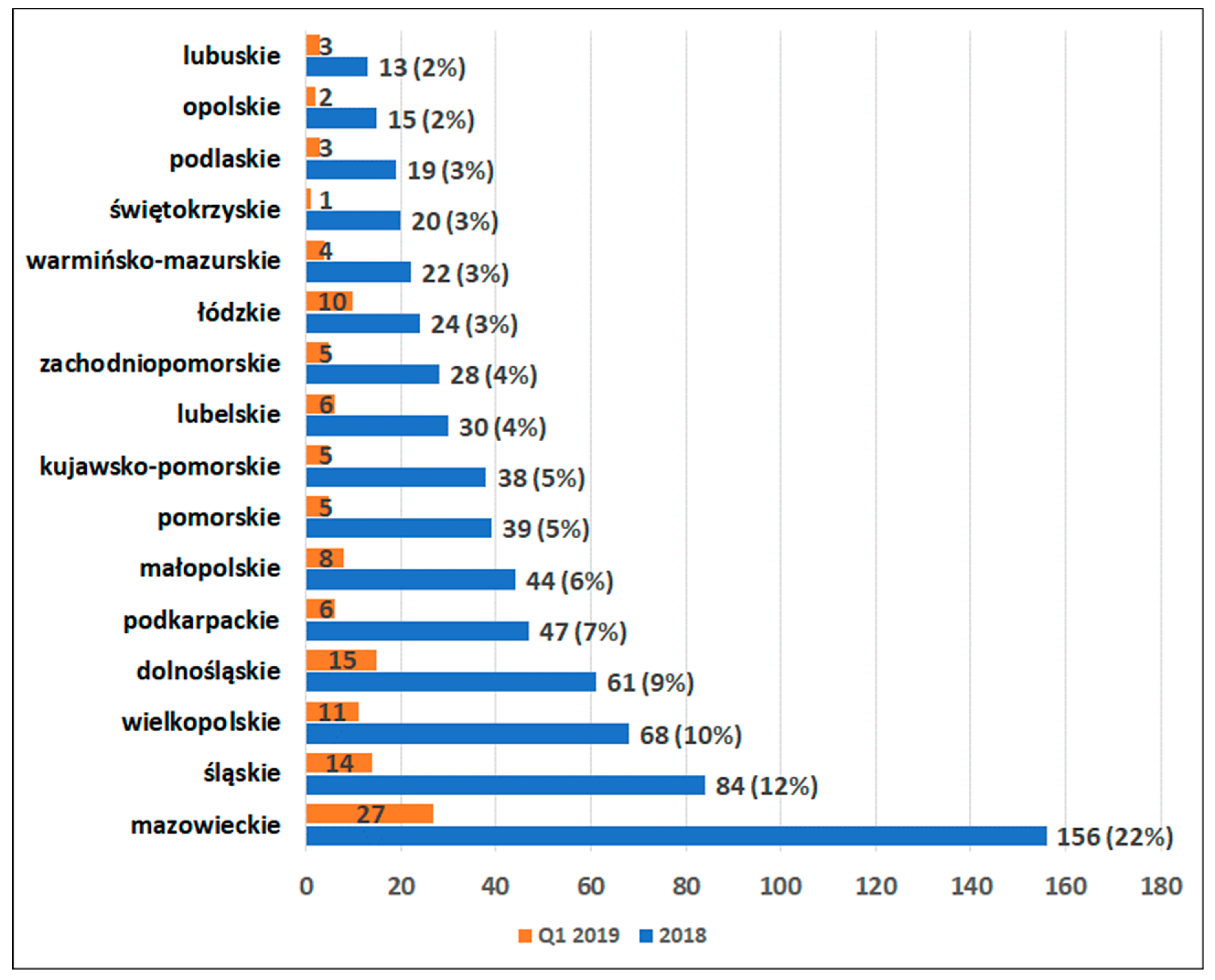
3.1. Statistical Description of Bankruptcies in Poland
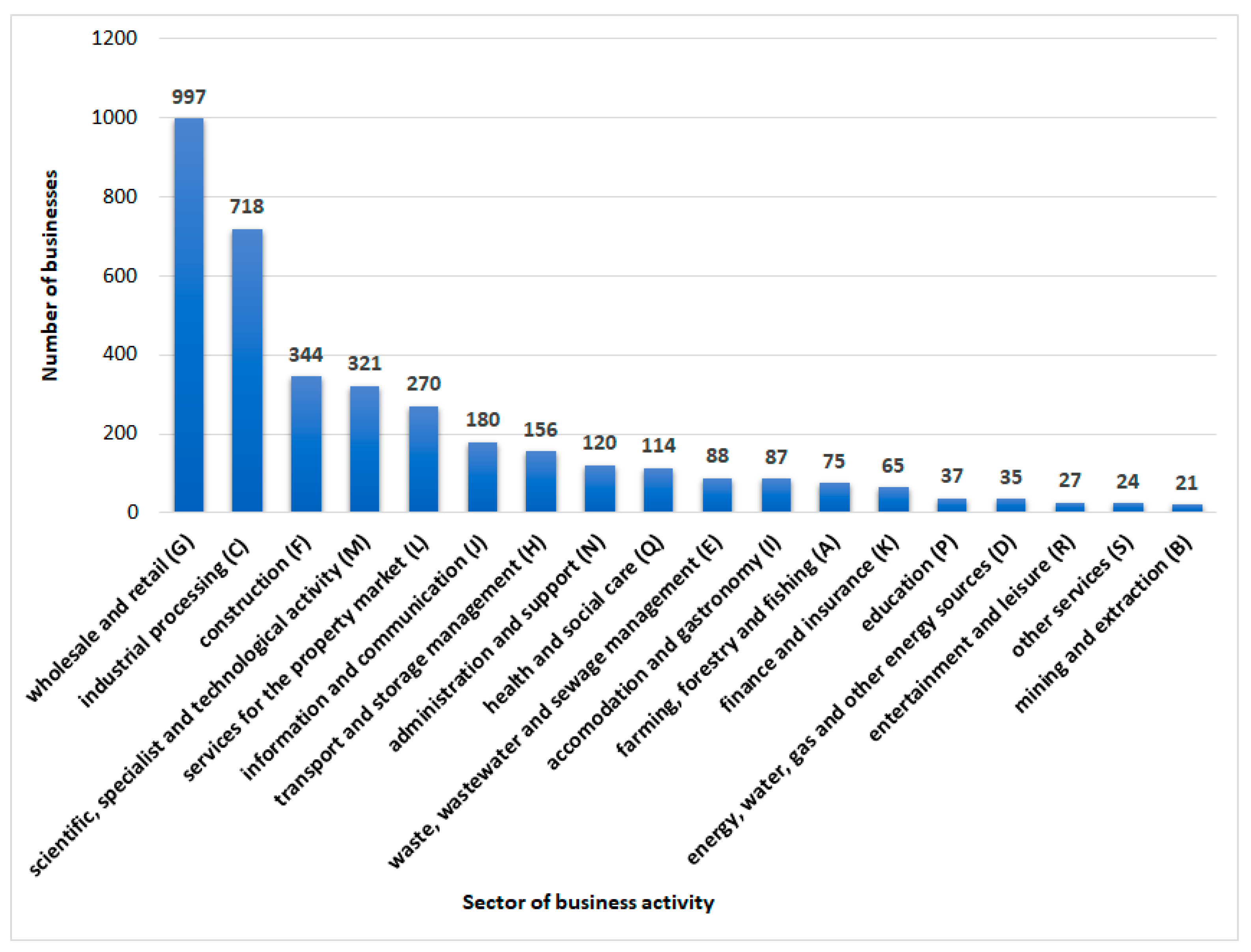
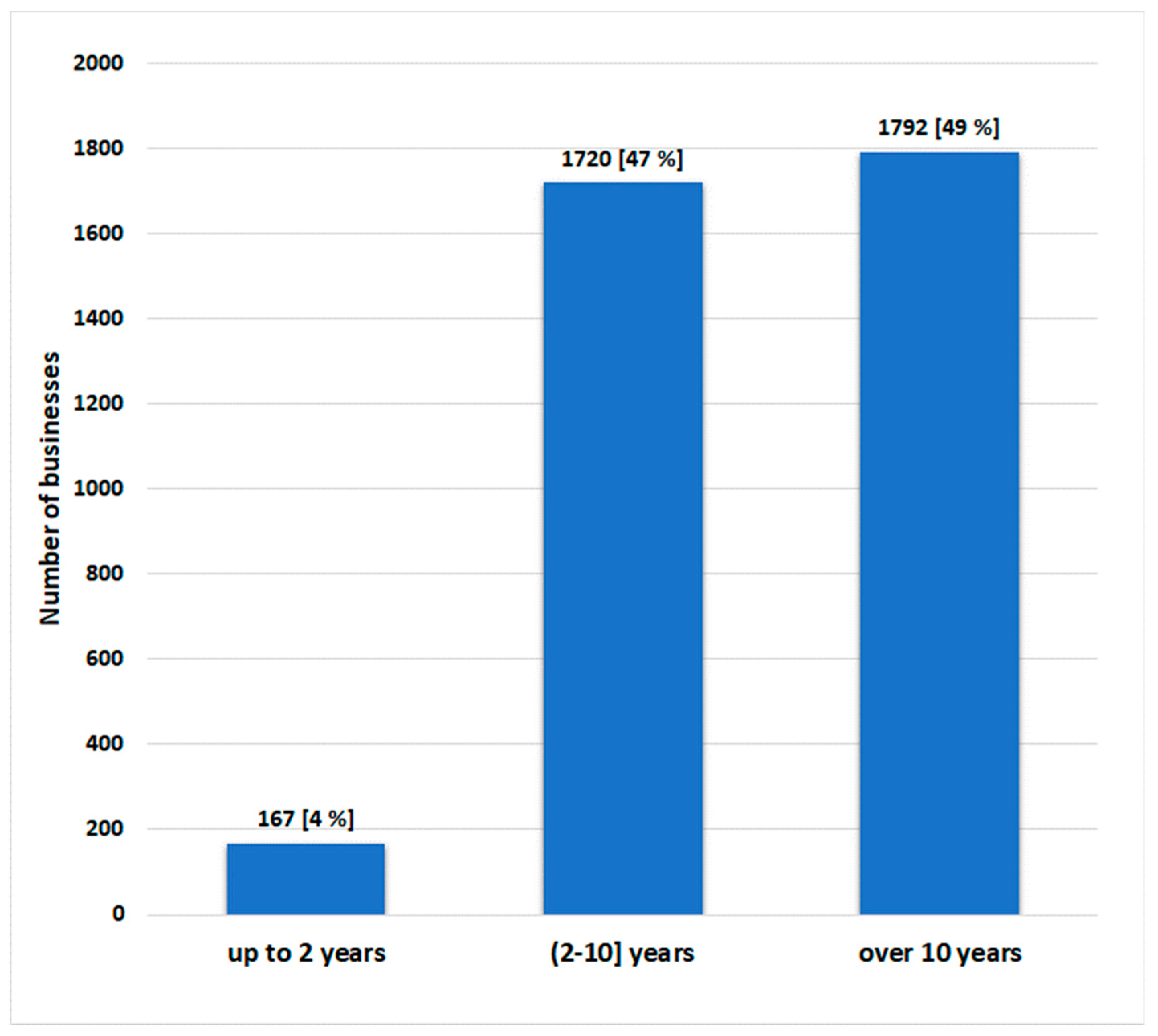
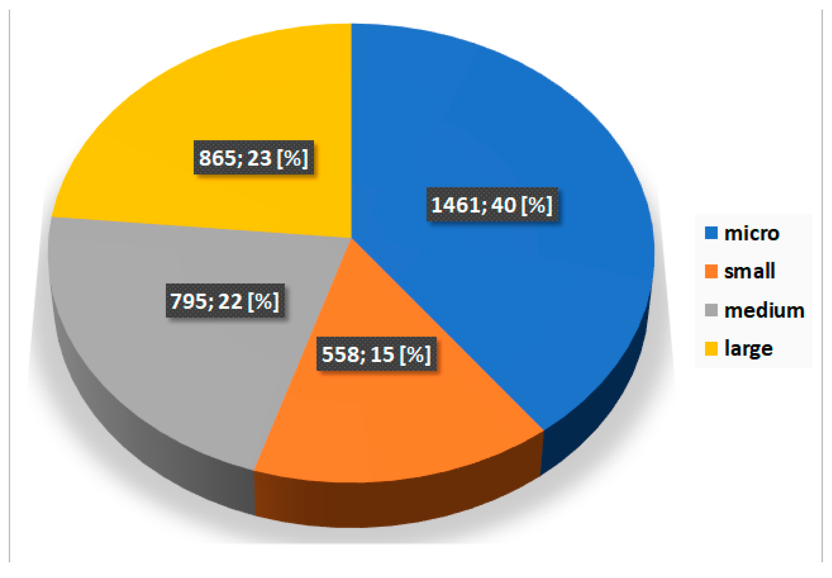
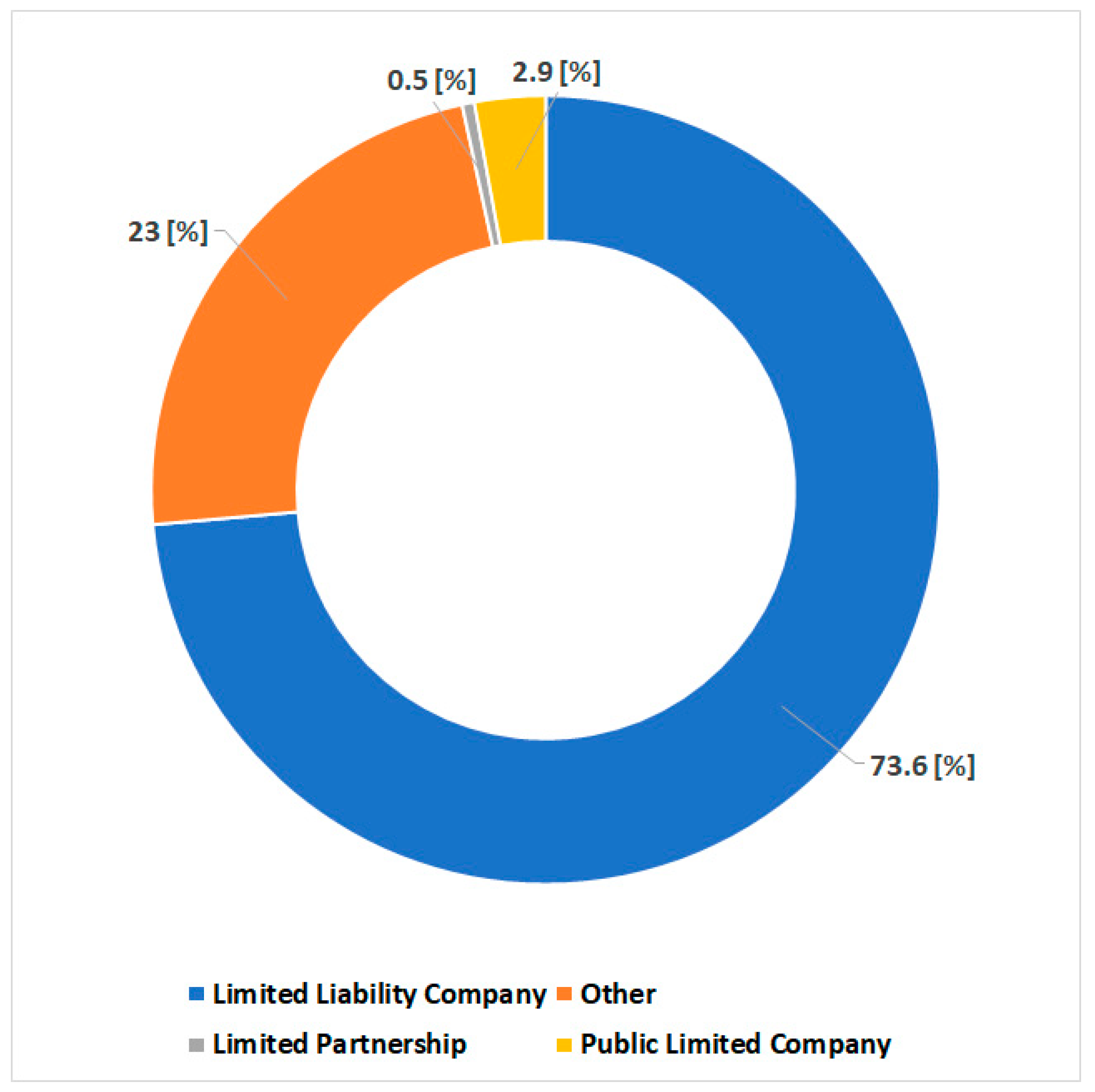
3.2. Characteristics of Companies Operating in the Podkarpackie Voivodeship
4. Materials and Methods
4.1. Ensemble Classifier Methodology
| Algorithm 1 AdaBoost.M1 algorithm |
|
| Algorithm 2 Bagging algorithm |
|
4.2. Feature Selection Process in Bankruptcy Prediction
| Algorithm 3 Genetic Algorithm Feature Selection (GAFS) |
|
4.3. Data Samples Description
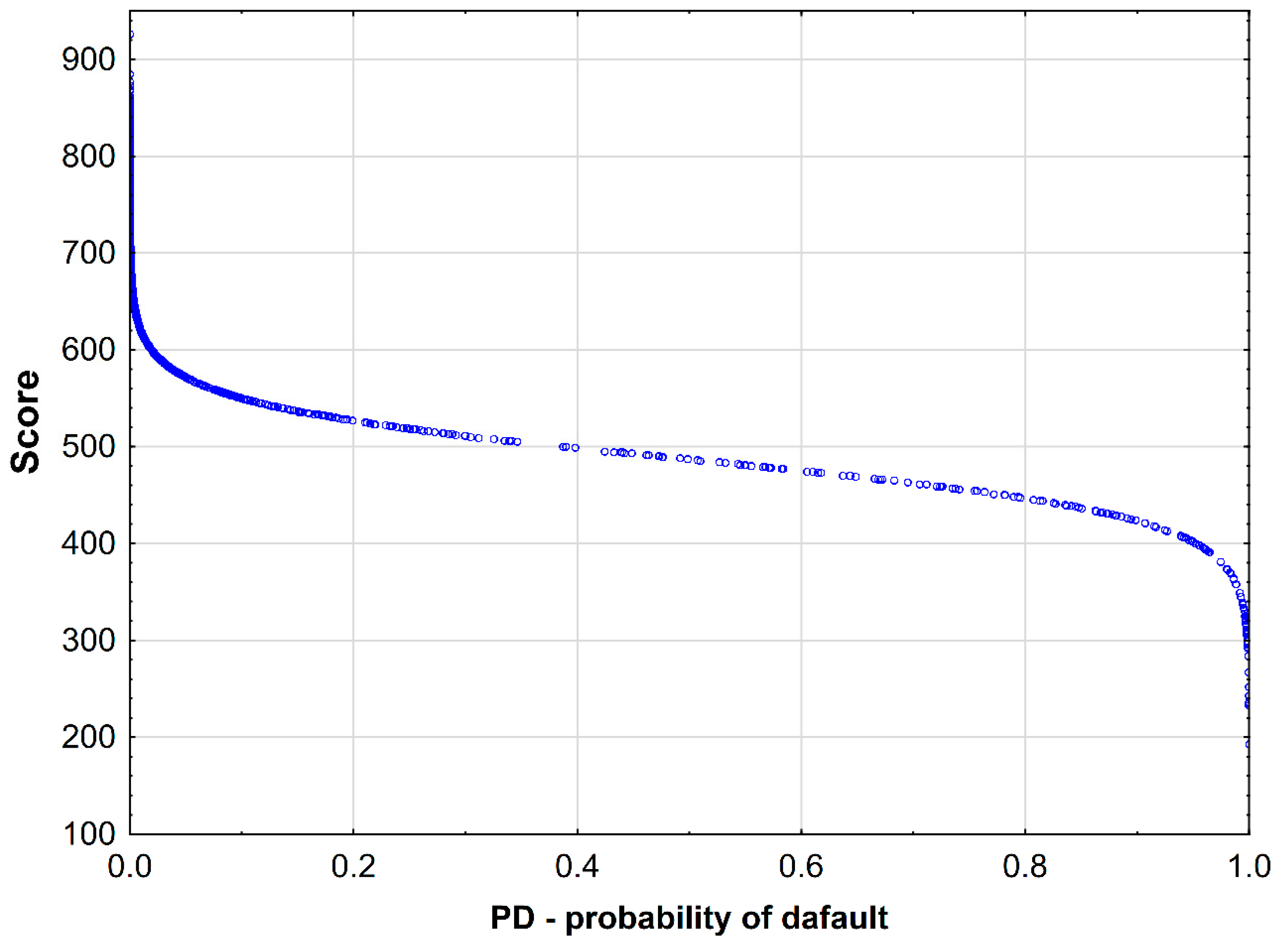
4.4. Procedure of Mapping PD into Scores
4.5. Validation Measures of Bankruptcy Prediction Models
4.6. Optimal Cut-Off Point for Scoring Determination
5. Research Results
- The choice of a suitable subset of financial ratios (bankruptcy predictors) determining the financial circumstances of the businesses analyzed (feature selection stage).
- Training and calibration of base models applied and ensemble models selected on the basis of the training sample. Determining the function of the probability of default and membership in forecast classes for both samples: training sample, and test and validation sample (which is not taken into account at the stage of calibration of the evaluated models).
- Determining the score value for the training sample and the test sample with a suitable scaling of the value of the resulting probability of default function for the estimated models and their transformation into corresponding resulting point score values.
- Validation of estimated models. Determining the values of validation statistics for the models applied and analysis of their discriminant capabilities for the training sample and the test sample. Selection of the best forecasting model.
- For the best model, determining the optimum cut-off point for the score value, i.e., the point below which a business should be categorized as bankrupt.
- Bankruptcy forecasts for analyzed businesses from the Podkarpackie Voivodeship in individual sectors of economic activity and business size. Final comparative analysis of results and final conclusions.
5.1. Feature Selection Stage—Selection of Ratios/Bankruptcy Risk Determinants
- Financial liquidity ratios: X1—Current ratio = Current assets to Short-term liabilities total (all liabilities with maturity shorter than one year): CA/STL, X2—Quick ratio = (Current assets − Inventories) to Short-term liabilities total: (CA-I)/STL, X3—Cash ratio = Cash and Cash equivalents to Short-term liabilities total: Cash/STL
- Profitability ratios: X4—Operating profit margin = Operating earnings to Net sales: OE/NS [%], X5—Return on assets (ROA) = Net profit (Total Revenue − Cost of Goods Sold − Operating Expenses − Other Expenses − Interest and Taxes) to Assets total (Balance sheet total): NP/BST [%], X6—Return on equity (ROE) = Net profit to Equity: NP/E [%], X7—Return on invested capital = Net profit to (Assets total − Short-term liabilities total): NP/(BST-STL) [%], X8—Net profitability = Net profit to Revenues from sales: NP/RS [%], X9—gross profit margin on sales = (Revenues from sales − Cost of goods sold) to Revenues from sales: (RS-CoGS)/RS [%], X10—operating return on assets = EBIT (Earnings Before Interest and Taxes) to Assets total: EBIT/BST [%]
- Debt ratios: X11—Overall debt = Liabilities total to Assets total (Balance sheet total): TL/BST [%], X12—Debt to equity = Liabilities total to Equity: (TL/E) [%], X13—Debt to EBITDA = Liabilities total to EBITDA: TL/EBITDA, X14—Financial leverage = Assets total (Balance sheet total) to Equity: BST/E [%]
- Management effectiveness ratios: X15—Receivable turnover = Revenues from sales to Short-term receivables: RS/STR, X16—Asset turnover = Revenues from sales to Assets total (Balance sheet total): RS/BST, X17—Inventory turnover = Revenues from sales to Inventories: RS/I, X18—Liability turnover = (Revenues from sales + Inventories) to Short-term liabilities total: (RS+I)/STL, X19—Working capital turnover = Revenues from sales to (Current assets − Short-term liabilities total): RS/(CA-STL)
- Capital structure ratios: X20—Structure of Equity to Assets total (Balance sheet total): E/BST [%], X21—Structure of Fixed assets to total assets (Balance sheet total): FA/BST [%], X22—Structure of Fixed assets to Current assets: FA/CA [%]
5.2. Calibration of the Parameters of Bankruptcy Risk Forecast Models (Calibration Stage)
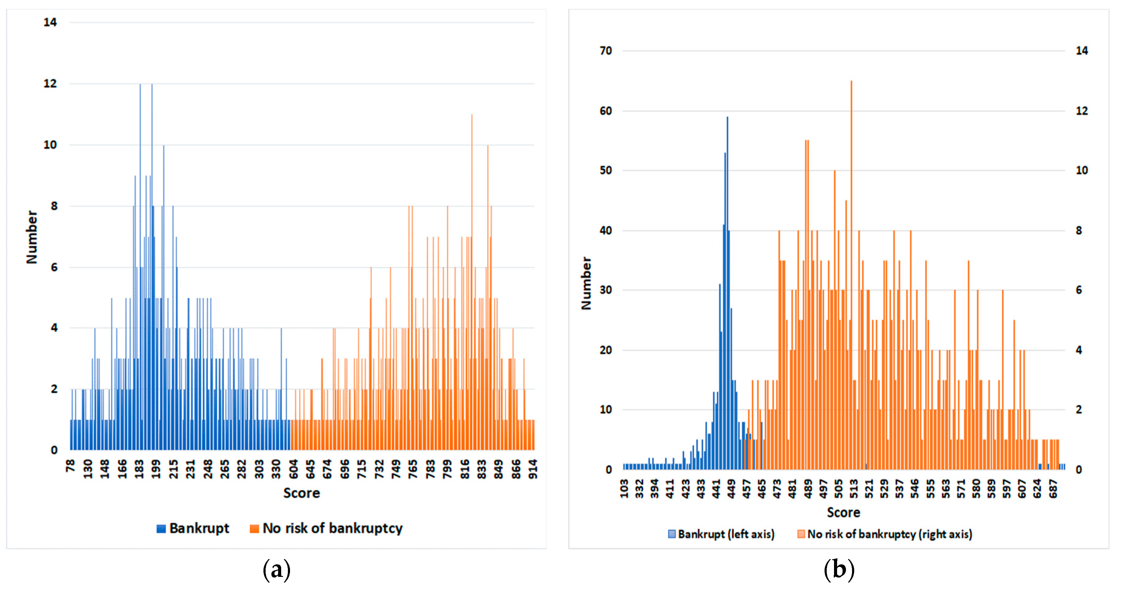
5.3. Determining Score for the Optimum Model (Score Scaling Stage)
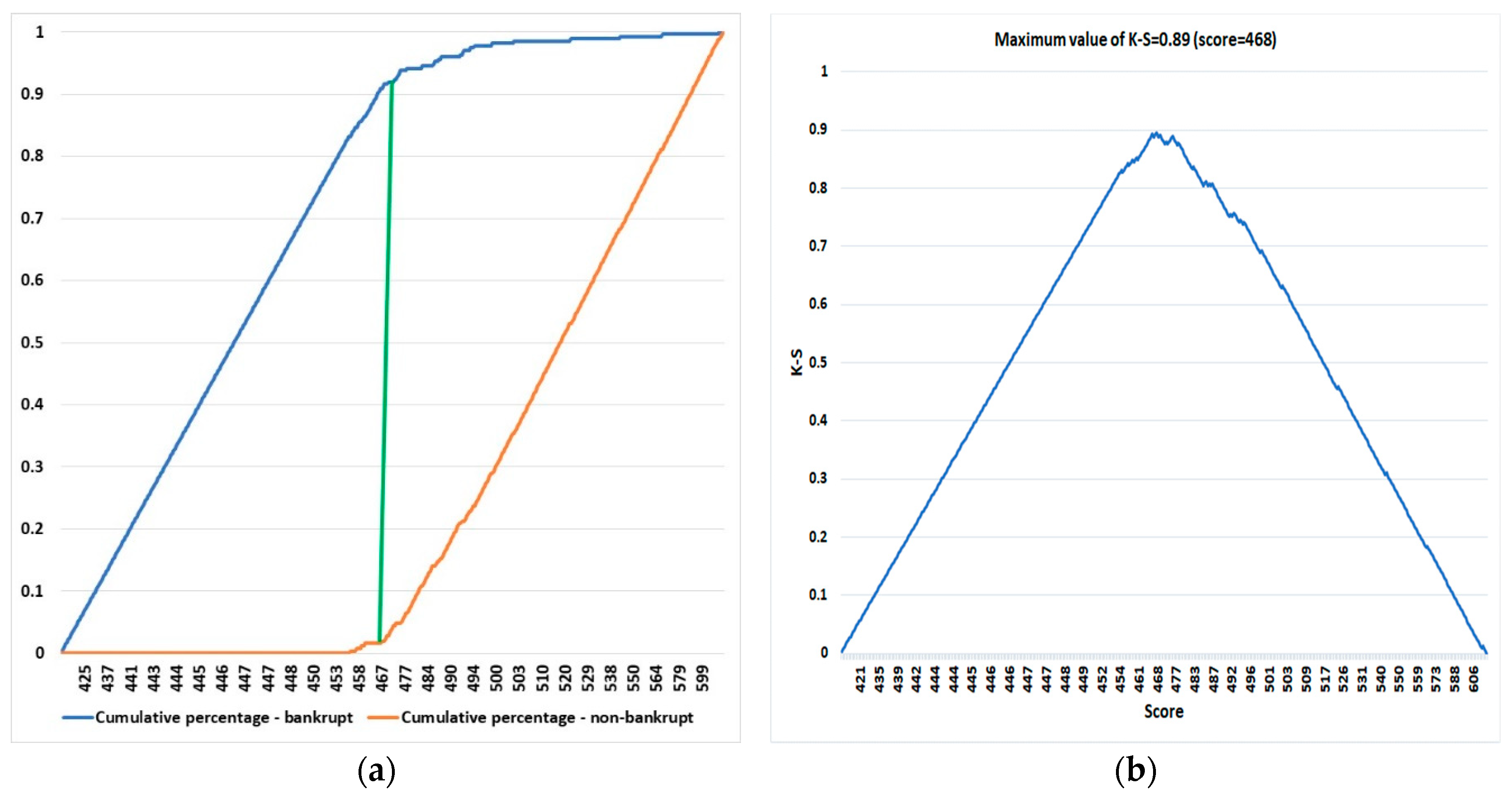
5.4. Model Validation (validation Stage)
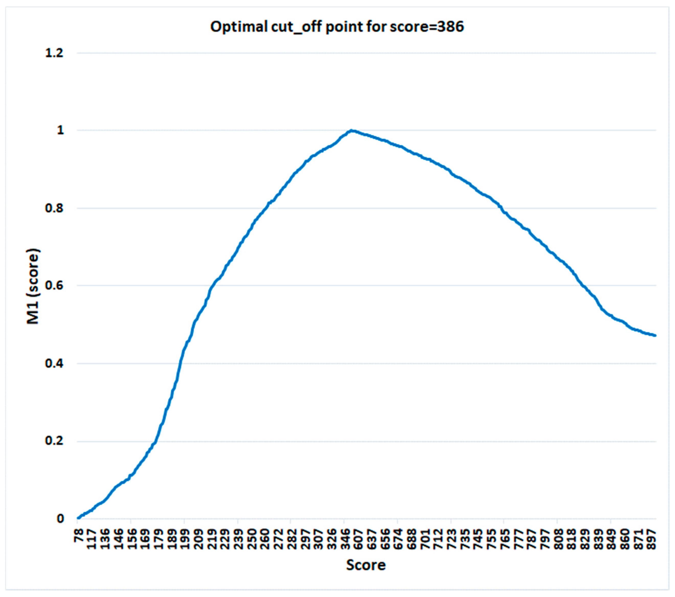
5.5. Optimal Cut_Off Point Determination Stage
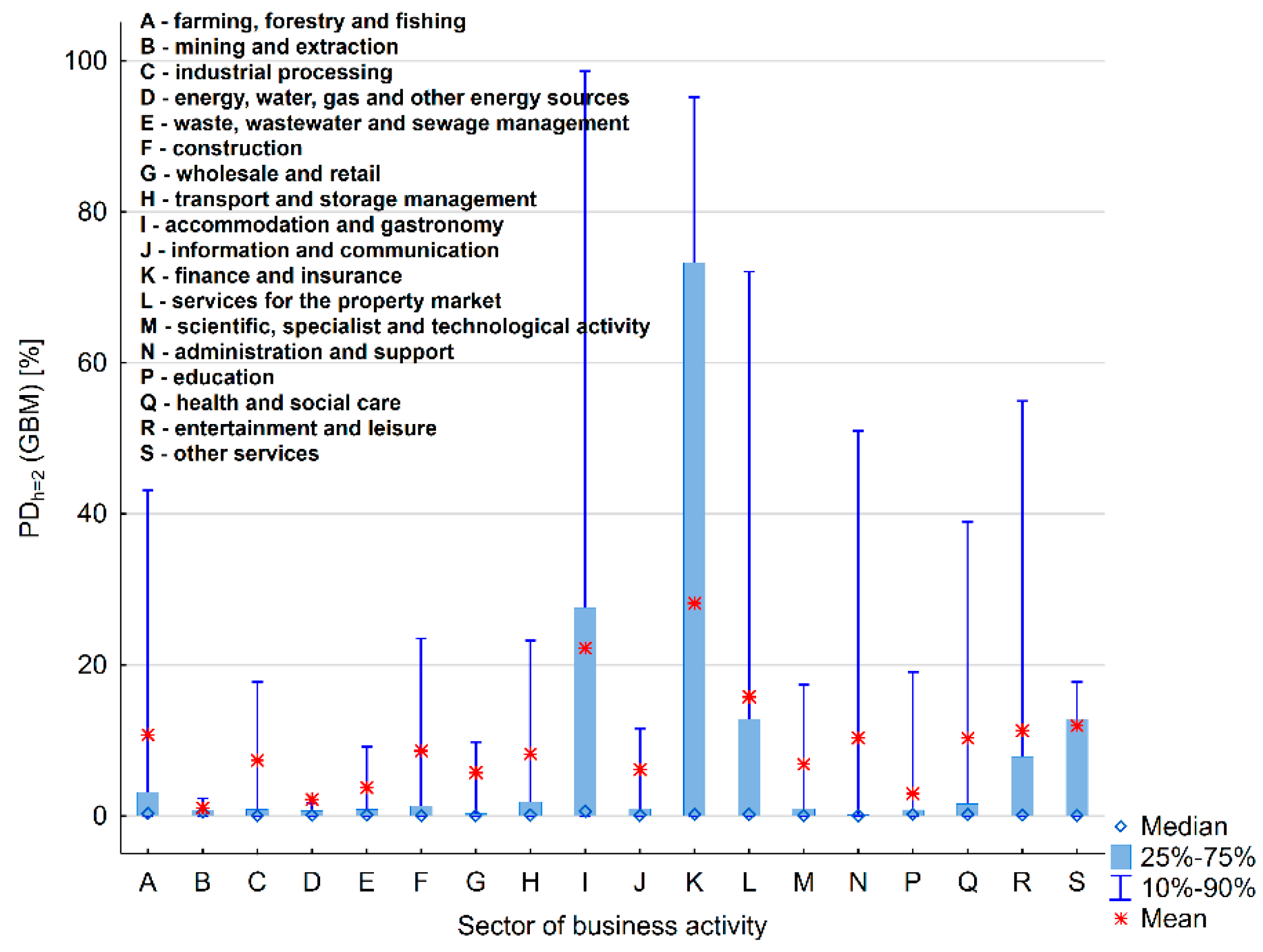
5.6. Classification of Enterprises from the Podkarpacie Region (Prediction Stage) Depending on the Risk of Their Bankruptcy
6. Discussion
7. Conclusions
- The scoring model designed for the early prediction of bankruptcy risk for Polish businesses from the Podkarpackie Voivodeship using ensemble classifiers was highly effective in forecasting and accurately evaluating the risk of default of the analyzed businesses.
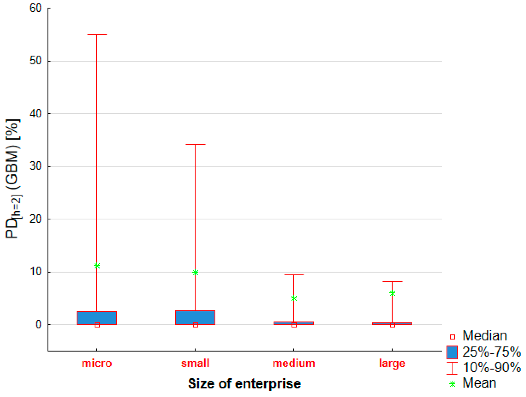
- An analysis of the forecast is obtained suggests that small enterprises are more exposed to risk of default than medium or large enterprises.
- The sector of business activity and unique characteristics of the economic activity influences a potentially higher risk of business bankruptcy. A higher number of potential bankruptcies is reported in some sectors of economic activity than in others.
- A higher risk of business bankruptcy for some particular industry branches may be caused the situation where bankruptcy models are sensitive to enterprises belonging to industry sectors. This can be considered as one of the limitations of the study presented in the paper. A potentially higher risk of business bankruptcy for some particular industry branches can be influenced by the model design. It would have to be examined in further research whether the estimated separate models for each sector would indicate lower values of PD and therefore lower exposure to the risk of bankruptcy of companies.
- Another limitation of the study is that bankruptcy models are sensitive to the phase of economic cycle (presented model does not cover it), but the influence of economic cycles on bankruptcy risk can be considered in further extensions of research.
- The approach presented in the paper can be used not only to assess the risk of bankruptcy of enterprises by market analysts and regional analysts, but also in banking activities to assess credit risk for corporate loans, where similar models are of course successfully implemented.
- The study may be extended in the future with an analysis and an assessment of the risk of bankruptcy for enterprises from other regions of Poland with the development of individual separate ensemble models for enterprises from key sectors of the country’s economy. It can also be extended to a comparative analysis of the risk of bankruptcy in given sectors of the economy for a group of countries, e.g., EU, Visegrad Group countries or the Three Seas Initiative countries.
Funding
Conflicts of Interest
Appendix A

| Classification Model Applied | Optimum Model Configuration (Training Sample) Parameter Selection Criterion: AUC (ROC) Sampling: (k = 5 fold) Cross-Validation |
|---|---|
| Model Parameters: | |
| Individual (single) classifier | |
| LDA (M1) linear discriminant analysis model | , , , , , , , , , , , , , |
| LOGIT (M2) logistic regression model | , , , , , , , , , , , |
| NNet (M3) neural network (single hidden layer network) | Network configuration: 19-5-1 Neuron activation function: logistic Error function = entropy fitting Calibrated parameter for weights: decay = 0.1 |
| SVM Radial (M4) Support Vector Machine | Cost parameter: C = 1 Hyper parameter: sigma = 11.969 |
| C&RT (M5) classification tree model | Tree complexity parameter (cp = 0.037) Tree split: (class: bankrupt) (class: no risk of bankruptcy) |
| MARS splines (M6) | product degree = 1 (degree of interaction); nprune = 12 (number of base functions); |
| Generalized Additive Model (GAM—M7) | Select = TRUE (feature selection); Link Function = Logit; Method = GCV.Cp (GCV method for an unknown parameter of model complexity) |
| Naive Bayes (M8) | Laplace Correction fL = 0 Distribution type usekernel = FALSE (Binomial) Bandwidth adjustment adjust = 1 |
| Ensemble meta-classifier (stacking) | |
| k-NN k-nearest neighbours, inputs: classification functions for base models (M1-M8) | Nearest neighbour parameter k = 9 |
| Ensemble classifier (boosting) | |
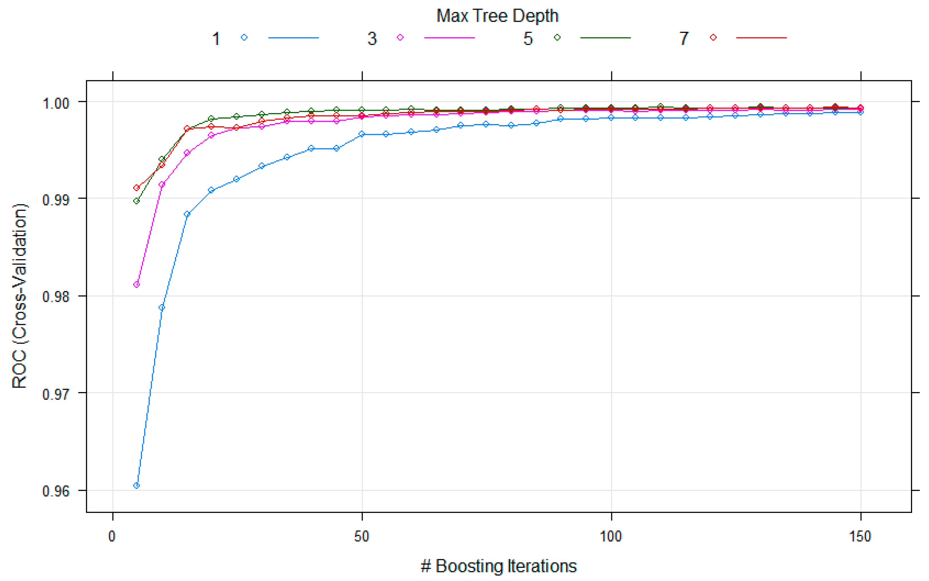
| Stochastic Gradient Boosting Machine (GBM) | Shrinkage = 0.2; n.minobsinnode = 15 (min. node size); n.trees = 130–boosting iterations interaction.depth = 5 (max. tree depth) |
| Boosted Logistic Regression (Logit Boost) | nIter = 13 (boosting iterations) |
| Ensemble classifier (bagging) | |
| Random Forest (RF) | mtry = 5 randomly selected predictors ntree = 500 (number of trees) |
| Averaged NNet (avNNet) | bag = TRUE; n = 5—bootstraps; size = 5—number of neurons in the hidden layer for component networks; decay = 0.9—decay parameter for weights; |
| Classification Model | Training Sample | ||||||
|---|---|---|---|---|---|---|---|
| AC | ACB | ACNB | AUCROC (GINI) | KS Statistics | Divergence (Div) | Information Value (IV) | |
| Base classifiers | |||||||
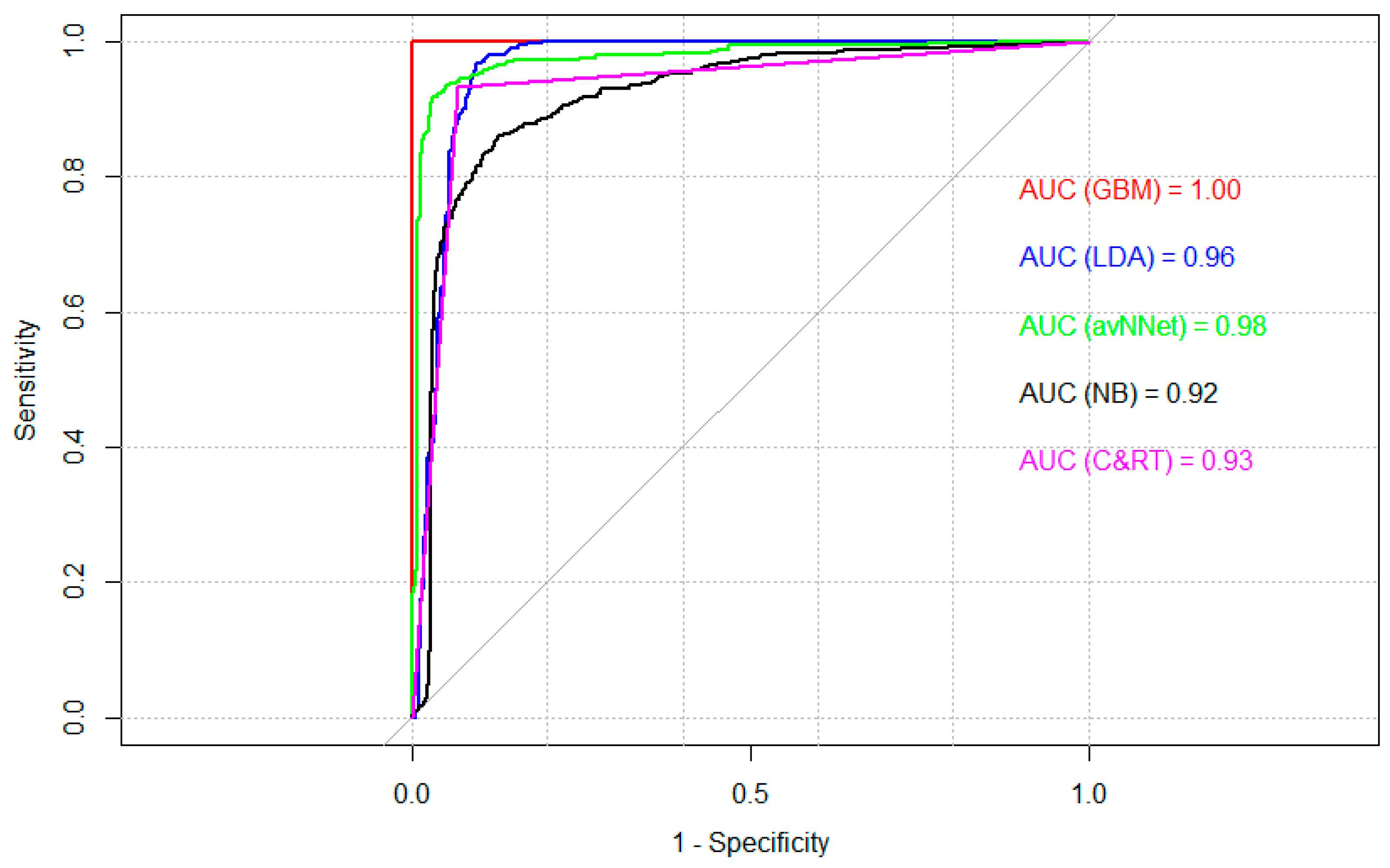
| Linear discriminant analysis (LDA)—M1 | 88.4 | 94.6 | 82.5 | 0.96 (0.92) | 0.87 | 2.6 | 5.2 |
| Logistic regression (Logit)—M2 | 96.8 | 96.1 | 97.6 | 0.97 (0.94) | 0.94 | 28.9 | 5.3 |
| Neural network (NNet)—M3 | 93.0 | 94.1 | 92.0 | 0.95 (0.90) | 0.86 | 7.5 | 5.2 |
| Support Vector Machine (SVM Radial—M4) | 96.4 | 95.4 | 97.4 | 0.99 (0.98) | 0.93 | 17.2 | 5.2 |
| Classification tree (C&RT)—M5 | 93.2 | 93.2 | 93.3 | 0.93 (0.86) | 0.87 | 11.9 | 5.2 |
| MARS splines—M6 | 96.0 | 95.8 | 96.3 | 0.99 (0.98) | 0.94 | 8.0 | 5.2 |
| Generalized Additive Model (GAM)—M7 | 97.7 | 98.0 | 97.4 | 0.99 (0.98) | 0.96 | 5.8 | 5.3 |
| Naive Bayes—M8 | 70.9 | 42.1 | 98.2 | 0.91 (0.82) | 0.73 | 1.0 | 5.2 |
| Ensemble classifier (stacking) | |||||||
| Meta-classifier ensemble: kNN—model results M1-M8 as inputs | 97.3 | 97.1 | 97.4 | 0.99 (0.98) | 0.96 | 23.0 | 5.3 |
| Ensemble classifiers (boosting) | |||||||
| Stochastic Gradient Boosting Machine (GBM) | 100 | 100 | 100 | 1.0 (1.0) | 1.0 | 92.1 | 5.3 |
| Logit Boost | 97.9 | 97.3 | 98.5 | 0.99 (0.98) | 0.96 | 20.5 | 5.3 |
| Ensemble classifiers (bagging) | |||||||
| Random Forest (RF) | 100 | 100 | 100 | 1.0 (1.0) | 1.0 | 6.4 | 5.3 |
| Averaged NNet (avNNet) | 94.0 | 94.6 | 93.4 | 0.98 (0.96) | 0.89 | 11.6 | 5.3 |
| Classification Model | Test Sample | ||||||
|---|---|---|---|---|---|---|---|
| AC | ACB | ACNB | AUCROC (GINI) | KS Statistics | Divergence (Div) | Information Value (IV) | |
| Base classifiers | |||||||
| Linear discriminant analysis (LDA)—M1 | 90.2 | 96.0 | 84.0 | 0.98 (0.96) | 0.89 | 11.8 | 7.1 |
| Logistic regression (Logit)—M2 | 96.5 | 94.5 | 98.8 | 0.97 (0.94) | 0.93 | 46.2 | 7.1 |
| Neural network (NNet)—M3 | 92.1 | 94.5 | 89.5 | 0.95 (0.90) | 0.86 | 11.2 | 7.1 |
| Support VectorMachine (SVM Radial)—M4 | 89.8 | 92.3 | 87.1 | 0.97 (0.94) | 0.82 | 10.8 | 7.1 |
| Classification tree (C&RT)—M5 | 94.2 | 95.2 | 93.1 | 0.94 (0.88) | 0.88 | 14.8 | 7.1 |
| MARS splines—M6 | 96.7 | 96.3 | 97.2 | 0.99 (0.98) | 0.95 | 41.7 | 7.1 |
| Generalized Additive Model (GAM)—M7 | 97.5 | 97.8 | 97.2 | 0.99 (0.98) | 0.96 | 43.0 | 7.1 |
| Naive Bayes—M8 | 68.4 | 41.7 | 97.6 | 0.93 (0.86) | 0.78 | 7.8 | 7.1 |
| Ensemble classifier (stacking) | |||||||
| Meta-classifier ensemble: kNN model result M1-M8 as inputs | 98.1 | 97.8 | 98.4 | 0.99 (0.98) | 0.97 | 22.2 | 7.1 |
| Ensemble classifiers (boosting) | |||||||
| Stochastic Gradient Boosting Machine (GBM) | 99.4 | 99.3 | 99.6 | 0.999 (0.998) | 0.99 | 57.6 | 7.1 |
| Logit Boost | 98.5 | 98.2 | 99.6 | 0.99 (0.98) | 0.98 | 20.6 | 7.1 |
| Ensemble classifiers (bagging) | |||||||
| Random Forest (RF) | 98.6 | 98.2 | 99.2 | 1.0 (1.0) | 0.98 | 4.5 | 7.1 |
| Averaged NNet (avNNet) | 93.8 | 96.0 | 91.5 | 0.97 (0.94) | 0.89 | 10.2 | 7.1 |
References
- Achim, Monica V., Codruta Mare, and Sorin N. Borlea. 2012. A statistical model of financial risk bankruptcy applied for Romanian manufacturing industry. Procedia Economics and Finance 3: 132–37. [Google Scholar] [CrossRef][Green Version]
- Agarwal, Vineet, and Richard Taffler. 2008. Comparing the performance of market-based and accounting-based bankruptcy prediction models. Journal of Banking & Finance 32: 1541–51. [Google Scholar]
- Ala’raj, Maher, and Maysam F. Abbod. 2016. Classifiers consensus system approach for credit scoring. Knowledge-Based Systems 104: 89–105. [Google Scholar] [CrossRef]
- Alaka, Hafiz A., Lukumon O. Oyedele, Hakeem A. Owolabi, Vikas Kumar, Saheed O. Ajayi, Olungbenga O. Akinade, and Muhammad Bilal. 2018. Systematic review of bankruptcy prediction models: Towards a framework for tool selection. Expert Systems with Applications 94: 164–84. [Google Scholar] [CrossRef]
- Alfaro, Esteban, Noelia Garcia, Matias Gamez, and David Elizondo. 2008. Bankruptcy forecasting: An empirical comparison of AdaBoost and neural networks. Decision Support Systems 45: 110–22. [Google Scholar] [CrossRef]
- Altman, Edward I. 1968. Financial ratios, discriminant analysis and the prediction of corporate bankruptcy. Journal of Finance 23: 589–609. [Google Scholar] [CrossRef]
- Anwar, Hina, Usman Qamar, and Abdul W. M. Qureshi. 2014. Global Optimization Ensemble Model for Classification Methods. The Scientific World Journal 2014: 1–9. [Google Scholar] [CrossRef]
- Barboza, Flavio, Herbert Kimura, and Edward Altman. 2017. Machine learning models and bankruptcy prediction. Expert Systems with Applications 83: 405–17. [Google Scholar] [CrossRef]
- Begley, Joy, Jin Ming, and Susan Watts. 1996. Bankruptcy classification errors in the 1980s: An empirical analysis of Altman’s and Ohlson’s models. Review of Accounting Studies 1: 267–84. [Google Scholar] [CrossRef]
- Breiman, Leo. 1996. Bagging predictors. Machine Learning 24: 123–40. [Google Scholar] [CrossRef]
- Breiman, Leo. 2001. Random Forests. Machine Learning 45: 5–32. [Google Scholar] [CrossRef]
- Brown, Iain, and Christophe Mues. 2012. An experimental comparison of classification algorithms for imbalanced credit scoring data sets. Expert Systems with Applications 39: 3446–53. [Google Scholar] [CrossRef]
- Bruneau, Catherine, Olivier de Brandt, and El A. Widad. 2012. Macroeconomic fluctuations and corporate financial fragility. Journal of Financial Stability 8: 219–35. [Google Scholar] [CrossRef]
- Chen, Yibing, Lingling Zhang, and Liang Zhang. 2013. Financial Distress Prediction for Chinese Listed Manufacturing Companies. Procedia Computer Science 17: 678–86. [Google Scholar] [CrossRef][Green Version]
- Chuang, Chun-Ling. 2013. Application of hybrid case-based reasoning for enhanced performance in bankruptcy prediction. Information Sciences 236: 174–85. [Google Scholar] [CrossRef]
- Cortes, Esteban A., Matias G. Martinez, and Noelia G. Rubio. 2007. A boosting approach for corporate failure prediction. Applied Intelligence 27: 29–37. [Google Scholar] [CrossRef]
- Diakomihalis, Mihail. 2012. The accuracy of Altman’s models in predicting hotel bankruptcy. International Journal of Accounting and Financial Reporting 2: 96–113. [Google Scholar] [CrossRef]
- Du Jardin, Philippe. 2018. Failure pattern-based ensembles applied to bankruptcy forecasting. Decision Support Systems 107: 64–77. [Google Scholar] [CrossRef]
- Emerging Markets Information Service (EMIS). 2019. EMIS Database. Available online: http://www.emis.com (accessed on 10 September 2019).
- Fedorova, Elena, Evgenii Gilenko, and Sergey Dovzhenko. 2013. Bankruptcy prediction for Russian companies: Application of combined classifiers. Expert Systems with Applications 40: 7285–93. [Google Scholar] [CrossRef]
- Freund, Yoav, and Robert E. Schapire. 1997. A decision theoretic generalization of online learning and an application to boosting. Journal of Computer and System Sciences 55: 119–39. [Google Scholar] [CrossRef]
- Friedman, Jerome H. 2002. Stochastic gradient boosting. Computational Statistics and Data Analysis 38: 367–78. [Google Scholar] [CrossRef]
- Główny Urząd Statystyczny (Statistics Poland). 2019. Bank Danych Lokalnych (Local Data Bank). Available online: https://bdl.stat.gov.pl (accessed on 10 September 2019).
- Hadasik, Dorota. 1998. The Bankruptcy of Enterprises in Poland and Methods of Its Forecasting. Poznań: Wydawnictwo Akademii Ekonomicznej w Poznaniu. [Google Scholar]
- Hamrol, Mirosław, and Jarosław Chodakowski. 2008. Prognozowanie zagrożenia finansowego przedsiębiorstwa. Wartość predykcyjna polskich modeli analizy dyskryminacyjnej. Badania Operacyjne i Decyzje 3: 17–32. [Google Scholar]
- Hastie, Trevor, Robert Tibshirani, and Jerome Friedman. 2013. The Elements of Statistical Learning: Data Mining, Inference, and Prediction. New York: Springer. [Google Scholar]
- Heo, Junyoung, and Jin Y. Yang. 2014. AdaBoost based bankruptcy forecasting of Korean construction companies. Applied Soft Computing 24: 494–99. [Google Scholar] [CrossRef]
- Hol, Suzan. 2007. The influence of the business cycle on bankruptcy probability. International Transactions in Operational Research 14: 75–90. [Google Scholar] [CrossRef]
- Hua, Zhongsheng, Yu Wang, Xiaoyan Xu, Bin Zhang, and Liang Liang. 2007. Predicting corporate financial distress based on integration of support vector machine and logistic regression. Expert Systems with Applications 33: 434–40. [Google Scholar] [CrossRef]
- Iturriaga, Felix J. L., and Ivan P. Sanz. 2015. Bankruptcy visualization and prediction using neural networks: A study of U.S. commercial banks. Expert Systems with Applications 42: 2857–69. [Google Scholar] [CrossRef]
- John, George H., Ron Kohavi, and Karl Pfleger. 1994. Irrelevant features and the subset selection problem. In Machine Learning Proceedings 1994. Proceedings of the Eleventh International Conference. Edited by William Cohen and Haym Hirsh. San Francisco: Morgan Kaufmann Publishers, pp. 121–29. [Google Scholar] [CrossRef]
- Jovic, Alan, Karla Brkic, and Nikola Bogunovic. 2015. A review of feature selection methods with applications. In 2015 38th International Convention on Information and Communication Technology, Electronics and Microelectronics. Edited by Peter Biljanovic, Z. Butkovic, K. Skala, B. Mikac, M. Cicin-Sain, V. Sruk, S. Ribaric, S. Gros, B. Vrdoljak, M. Mauher and et al. New York: IEEE, pp. 1200–5. [Google Scholar] [CrossRef]
- Karas, Michal, Maria Reznakova, and Petr Pokorny. 2017. Predicting bankruptcy of agriculture companies: Validating selected models. Polish Journal of Management Studies 15: 110–20. [Google Scholar] [CrossRef]
- Kim, Hyunjoon, and Zheng Gu. 2010. A Logistic Regression Analysis for Predicting Bankruptcy in the Hospitality Industry. Journal of Hospitality Financial Management 14: 17–34. [Google Scholar] [CrossRef]
- Kim, Myoung-Jong, and Dae-Ki Kang. 2010. Ensemble with neural networks for bankruptcy prediction. Expert Systems with Applications 37: 3373–79. [Google Scholar] [CrossRef]
- Kim, Myoung-Jong, Dae-Ki Kang, and Hong B. Kim. 2015. Geometric mean based boosting algorithm with over-sampling to resolve data imbalance problem for bankruptcy prediction. Expert Systems with Applications 42: 1074–82. [Google Scholar] [CrossRef]
- Kliestik, Tomas, Jana Kliestikova, Maria Kovacova, Lucia Svabova, Katarina Valaskova, Marek Vochozka, and Judit Olah. 2018. Prediction of Financial Health of Business Entities in Transition Economies. New York: Addleton Academic Publishers. [Google Scholar]
- Korol, Tomasz. 2010. Early Warning Systems of Enterprises to the Risk of Bankruptcy. Warsaw: Wolters Kluwer. [Google Scholar]
- Kuhn, Max, and Kjell Johnson. 2013. Applied Predictive Modeling. New York: Springer. [Google Scholar]
- Kumar, Ravi P., and Vadlamani Ravi. 2007. Bankruptcy prediction in banks and firms via statistical and intelligent techniques—A review. European Journal of Operational Research 180: 1–28. [Google Scholar] [CrossRef]
- Lessmann, Stefan, Bart Baesens, Hsin-Vonn Seow, and Lyn C. Thomas. 2015. Benchmarking state-of-the-art classification algorithms for credit scoring: An update of research. European Journal of Operational Research 247: 124–36. [Google Scholar] [CrossRef]
- Li, Hui, and Jie Sun. 2012. Case-based reasoning ensemble and business application: A computational approach from multiple case representations driven by randomness. Expert Systems with Applications 39: 3298–310. [Google Scholar] [CrossRef]
- Mączyńska, Elżbieta. 1994. Assessment of the condition of the enterprise. Simplified methods. Życie Gospodarcze 38: 42–45. [Google Scholar]
- Marcinkevicius, Rosvydas, and Rasa Kanapickiene. 2014. Bankruptcy prediction in the sector of construction in Lithuania. Procedia—Social and Behavioral Sciences 156: 553–57. [Google Scholar] [CrossRef]
- Ogólnopolski Monitor Upadłościowy (Coface Polish National Bankruptcy Monitor). 2019. Available online: http://www.coface.pl/en (accessed on 10 September 2019).
- Ohlson, James A. 1980. Financial ratios and the probabilistic prediction of bankruptcy. Journal of Accounting Research 18: 109–31. [Google Scholar] [CrossRef]
- Prusak, Błażej. 2005. Nowoczesne Metody Prognozowania Zagrożenia Finansowego Przedsiębiorstw. Warsaw: Wydawnictwo Difin. [Google Scholar]
- Ptak-Chmielewska, Aneta. 2016. Statistical models for corporate credit risk assessment—Rating models. Acta Universitatis Lodziensis Folia Oeconomica 3: 98–111. [Google Scholar] [CrossRef]
- Rajin, Danica, Danijela Milenkovic, and Tijana Radojevic. 2016. Bankruptcy prediction models in the Serbian agricultural sector. Economics of Agriculture 1: 89–105. [Google Scholar] [CrossRef]
- Siddiqi, Naeem. 2017. Intelligent Credit Scoring, 2nd ed. Hoboken: John Wiley & Sons. [Google Scholar]
- Stowarzyszenie Dolina Lotnicza (Aviation Valley Association). 2019. Available online: http://www.dolinalotnicza.pl/en/business-card (accessed on 10 September 2019).
- Sun, Jie, Hamido Fujita, Peng Chen, and Hui Li. 2017. Dynamic financial distress prediction with concept drift based on time weighting combined with AdaBoost support vector machine ensemble. Knowledge-Based Systems 120: 4–14. [Google Scholar] [CrossRef]
- Thomas, Lyn C. 2009. Consumer Credit Models. New York: Oxford University Press. [Google Scholar]
- Topaloglu, Zeynep. 2012. A Multi-period Logistic Model of Bankruptcies in the Manufacturing Industry. International Journal of Finance and Accounting 1: 28–37. [Google Scholar] [CrossRef]
- Tsai, Chih-Fong, and Yu-Feng Hsu. 2013. A meta-learning framework for bankruptcy prediction. Journal of Forecasting 32: 167–79. [Google Scholar] [CrossRef]
- Tsai, Chih-Fong, and Jhen-Wei Wu. 2008. Using neural network ensembles for bankruptcy prediction and credit scoring. Expert Systems with Applications 34: 2639–49. [Google Scholar] [CrossRef]
- Tsai, Chih-Fong, Yu-Feng Hsu, and David C. Yen. 2014. A comparative study of classifier ensembles for bankruptcy prediction. Applied Soft Computing 24: 977–84. [Google Scholar] [CrossRef]
- Twala, Bhekisipho. 2010. Multiple classifier application to credit risk assessment. Expert Systems with Applications 37: 3326–36. [Google Scholar] [CrossRef]
- Vlamis, Prodromos. 2007. Default Risk of the UK Real Estate Companies: Is There a Macro-economy Effect? The Journal of Economic Asymmetries 4: 99–117. [Google Scholar] [CrossRef]
- West, David, Scott Dellana, and Jingxia Qian. 2005. Neural network ensemble strategies for financial decision applications. Computers & Operations Research 32: 2543–59. [Google Scholar]
- Wolpert, David H. 1992. Stacked generalization. Neural Networks 5: 241–59. [Google Scholar] [CrossRef]
- Youn, Hyewon, and Zheng Gu. 2010. Predict US restaurant fi rm failures: The artificial neural network model versus logistic regression model. Tourism and Hospitality Research 10: 171–87. [Google Scholar] [CrossRef]
- Zhang, Cha, and Yunqian Ma. 2012. Ensemble Machine Learning. Methods and Applications. New York: Springer. [Google Scholar]
- Zhang, Defu, Xiyue Zhou, Stephen C. H. Leung, and Jiemin Zheng. 2010. Vertical bagging decision trees model for credit scoring. Expert Systems with Applications 37: 7838–43. [Google Scholar] [CrossRef]
- Zhou, Zhi-Hua. 2012. Ensemble Methods. Foundations and Algorithms. Boca Raton: CRC Press. [Google Scholar]
- Zięba, Maciej, Sebastian K. Tomczak, and Jakub M. Tomczak. 2016. Ensemble boosted trees with synthetic features generation in application to bankruptcy prediction. Expert Systems with Applications 58: 93–101. [Google Scholar] [CrossRef]
- Zweig, Mark H., and Gregory Campbell. 1993. Receiver-Operating Characteristic (ROC) plots: A fundamental evaluation tool in clinical medicine. Clinical Chemistry 39: 561–77. [Google Scholar] [CrossRef] [PubMed]


| Methods Used in Forecasting Business Bankruptcy Risk | ||
|---|---|---|
| Conventional Approach Based on Single Classifiers | Ensemble Classifiers | |
| Statistical Methods | Non-Statistical Methods and Machine Learning | |
| Logistic regression (LOGIT) | Mathematical programming | Stacking:
|
| Linear discriminant analysis (LDA) | Expert systems | Boosting (e.g.):
|
| Classification and Regression Trees (C&RT) | Neural networks (NNet) | Bagging (e.g.):
|
| Nearest Neighbor algorithm (k-NN) k-Nearest Neighbors | Support Vector Machine (SVM) | |
| Naive Bayes classifier (NB) | Generalized Additive Models (GAM) | |
| Multivariate Adaptive Regression Splines (MARS) | ||
| ReportedBankruptcy | Forecast Bankruptcy | |
|---|---|---|
| B | NB | |
| B (negative class: bankrupt) | TN (True Negative) | FN (False Negative) |
| NB (positive class: non-bankrupt) | FP (False Positive) | TP (True Positive) |
| Ratio | Discriminant Measures | ||
|---|---|---|---|
| IV | GINI | V-Cramer | |
| X9 (Z8)—Return On Sales (profit margin) (gross) [%] | 5.81 | 0.86 | 0.84 |
| X11 (Z10)—Overall Debt [%] | 4.82 | 0.88 | 0.87 |
| X12 (Z11)—Debt to Equity [%] | 4.04 | 0.81 | 0.79 |
| X13 (Z12)—Debt/EBITDA | 2.76 | 0.72 | 0.66 |
| X5 (Z4)—Return on Assets (ROA) [%] | 1.66 | 0.68 | 0.60 |
| X8 (Z7)—Net Profit Margin [%] | 1.62 | 0.67 | 0.58 |
| X10 (Z9)—Operating Return on Assets [%] | 1.59 | 0.66 | 0.57 |
| X4 (Z3)—Operating Profit Margin [%] | 1.57 | 0.66 | 0.57 |
| X7 (Z6)—Return On Invested Capital [%] | 1.40 | 0.65 | 0.55 |
| X20 (Z18)—Equity To Total Assets Structure [%] | 1.39 | 0.65 | 0.55 |
| X6 (Z5)—Return On Equity ROE [%] | 1.18 | 0.63 | 0.51 |
| X18 (Z16)—Liability Turnover | 0.93 | 0.61 | 0.46 |
| X21 (Z19)—Fixed Assets to Total Assets Structure [%] | 0.89 | 0.57 | 0.38 |
| X17 (Z15)—Inventory turnover | 0.75 | 0.59 | 0.42 |
| X15 (Z13)—Receivable Turnover | 0.72 | 0.58 | 0.40 |
| X19 (Z17)—Working Capital Turnover | 0.66 | 0.58 | 0.39 |
| X3 (Z2)—Cash Ratio | 0.66 | 0.58 | 0.39 |
| X1 (Z1)—Current Ratio | 0.59 | 0.57 | 0.37 |
| X16 (Z14)—Asset Turnover | 0.28 | 0.52 | 0.22 |
| Sector | Number of Businesses Forecast by the Ensemble Scoring Model in a Given Bankruptcy Risk Class (h = 2 years, until 2020) | ||
|---|---|---|---|
| Bankrupt (B) | Uncertain (“Grey Zone”) | Healthy (No Risk of Bankruptcy) (NB) | |
| A—farming, forestry and fishing | 2 (4%) (small = 1; medium = 1) | 3 (6%) (micro = 1; small = 1; large = 1) | 45 (90%) (micro = 10; small = 12; medium = 10; large = 13) |
| B—mining and extraction | 0 | 0 | 12 (100%) (micro = 4; small = 1; medium = 4; large = 3) |
| C—industrial processing | 11 (2%) (micro = 1; small = 4; medium = 5; large = 1) | 27 (5%) (micro = 6; small = 9; medium = 3; large = 9) | 543 (93%) (micro = 84; small = 83; medium = 175; large = 201) |
| D—energy, water, gas and other energy sources | 0 | 0 | 25 (100%) (micro = 4; small = 3; medium = 6; large = 12) |
| E—waste, wastewater and sewage management | 0 | 2 (3%) (small = 1; medium = 1) | 65 (97%) (micro = 11; small = 5; medium = 18; large = 31) |
| F—construction | 7 (3%) (micro = 2; small = 1; medium = 2; large = 2) | 10 (5%) (micro = 9; large = 1) | 203 (92%) (micro = 55; small = 44; medium = 52; large = 52) |
| G—wholesale and retail | 17 (2%) (micro = 9; small = 3; large = 5) | 19 (3%) (micro = 5; small = 4; medium = 5; large = 1) | 698 (95%) (micro = 185; small = 121; medium = 226; large = 166) |
| H—transport and storage management | 2 (3%) (micro = 1; small = 1) | 3 (4%) (small = 1; large = 2) | 70 (93%) (micro = 18; small = 10; medium = 20; large = 22) |
| I—accommodation and gastronomy | 7 (13%) (micro = 4; medium = 2; large = 1) | 4 (7%) (micro = 1; medium = 2; large = 1) | 45 (80%) (micro = 17; small = 8; medium = 6; large = 14) |
| J—information and communication | 0 | 3 (5%) (micro = 3) | 52 (95%) (micro = 16; small = 7; medium = 11; large = 18) |
| K—finance and insurance | 0 | 4 (33%) (micro = 1; small = 2; large = 1) | 8 (67%) (small = 2; medium = 4; large = 2) |
| L—services for the property market | 2 (3%) (micro = 1; small = 1) | 10 (14%) (micro = 5; small = 2; medium = 2; large = 1) | 61 (83%) (micro = 20; small = 8; medium = 12; large = 21) |
| M—scientific, specialist and technological activity | 1 (2%) (micro = 1) | 2 (3%) (micro = 1; large = 1) | 58 (95%) (micro = 24; small = 8;medium = 14; large = 12) |
| N—administration and support | 2 (5%) (micro = 2) | 3 (7%) (micro = 1; large = 2) | 38 (88%) (micro = 11; small = 3; medium = 8; large = 16) |
| P—education | 0 | 0 | 9 (100%) (micro = 1; small = 2; medium = 2; large = 4) |
| Q—health and social care | 1 (3%) (large = 1) | 2 (5%) (small = 1; large = 1) | 35 (92%) (micro = 10; small = 5; medium = 8; large = 12) |
| R—entertainment and leisure | 0 | 2 (18%) (micro = 2) | 9 (82%) (micro = 5; small = 2; medium = 2) |
| S—other services | 0 | 1 (9%) (micro = 1) | 10 (91%) (micro = 3; medium = 5; large = 2) |
| Total | 52 (2%) micro = 4%; small = 3%; medium = 2%; large = 2% | 95 (5%) micro = 7%; small = 6%; medium = 2%; large = 4% | 1986 (93%) micro = 89%; small = 91%; medium = 96%; large = 94% |
| Reported Bankruptcy | Forecast Bankruptcy (h = 2 years) to 2020 | ||
|---|---|---|---|
| Bankrupt | Uncertain (Potentially Bankrupt) | Healthy (No Risk of Bankruptcy) | |
| Bankrupt | 31 (79%) | 3 (8%) | 5 (13%) |
| No risk of bankruptcy | 21 (1%) | 92 (4%) | 1981 (95%) |
© 2020 by the author. Licensee MDPI, Basel, Switzerland. This article is an open access article distributed under the terms and conditions of the Creative Commons Attribution (CC BY) license (http://creativecommons.org/licenses/by/4.0/).
Share and Cite
Pisula, T. An Ensemble Classifier-Based Scoring Model for Predicting Bankruptcy of Polish Companies in the Podkarpackie Voivodeship. J. Risk Financial Manag. 2020, 13, 37. https://doi.org/10.3390/jrfm13020037
Pisula T. An Ensemble Classifier-Based Scoring Model for Predicting Bankruptcy of Polish Companies in the Podkarpackie Voivodeship. Journal of Risk and Financial Management. 2020; 13(2):37. https://doi.org/10.3390/jrfm13020037
Chicago/Turabian StylePisula, Tomasz. 2020. "An Ensemble Classifier-Based Scoring Model for Predicting Bankruptcy of Polish Companies in the Podkarpackie Voivodeship" Journal of Risk and Financial Management 13, no. 2: 37. https://doi.org/10.3390/jrfm13020037
APA StylePisula, T. (2020). An Ensemble Classifier-Based Scoring Model for Predicting Bankruptcy of Polish Companies in the Podkarpackie Voivodeship. Journal of Risk and Financial Management, 13(2), 37. https://doi.org/10.3390/jrfm13020037