Early Warning Signs of Financial Market Turmoils

Abstract

Volatility clustering and fat tails are prominently observed in financial markets. Here, we analyze the underlying mechanisms of three agent-based models explaining these stylized facts in terms of market instabilities and compare them on empirical grounds. To this end, we first develop a general framework for detecting tail events in stock markets. In particular, we introduce Hawkes processes to automatically identify and date onsets of market turmoils which result in increased volatility. Second, we introduce three different indicators to predict those onsets. Each of the three indicators is derived from and tailored to one of the models, namely quantifying information content, critical slowing down or market risk perception. Finally, we apply our indicators to simulated and real market data. We find that all indicators reliably predict market events on simulated data and clearly distinguish the different models. In contrast, a systematic comparison on the stocks of the Forbes 500 companies shows a markedly lower performance. Overall, predicting the onset of market turmoils appears difficult, yet, over very short time horizons high or rising volatility exhibits some predictive power.

1. Introduction

Financial market prices are vastly fluctuating with prices occasionally rallying upwards and suddenly collapsing back down. The notion of “excess volatility” has been coined as price fluctuations often not being able to be reconciled with changes in economic fundamentals (Shiller 2005). On the contrary, volatility, i.e., the standard deviation of returns, appears to exhibit a dynamics of its own, exhibiting temporal clustering and long-range dependence (Chakraborti et al. 2011; Cont 2001). Econophysics has since developed and proposed models which explain these and other stylized facts of volatility in terms of endogenous dynamics arising from the collective action of many heterogeneous traders (Aymanns and Farmer 2015; Franke and Westerhoff 2016; Lux and Marchesi 1999; Patzelt and Pawelzik 2013; Samanidou et al. 2007).

According to this view, market fluctuations are amplified by feedbacks inherent in the dynamics of traders, e.g., arising from chartist strategies (Lux and Marchesi 1999), herding (Franke and Westerhoff 2016) or leverage targeting (Aymanns and Farmer 2015). While these models can replicate several stylized facts, their empirical estimation and analysis remains challenging. Yet, according to these models, especially large market fluctuations are driven by dynamical instabilities and could potentially be preceded by specific statistical signatures such as critical slowing down. While critical slowing down has successfully been used as an early warning sign from physics to ecology (see Scheffer et al. (2012) and references therein), complex systems thinking is still not widespread among economic scientists and practitioners. Nevertheless, some anecdotal evidence, i.e., focusing on crisis periods alone without a systematic investigation of predictive performance, has found that rising volatility might provide an early warning sign of financial crises (Diks et al. 2018; Guttal et al. 2016). In contrast, within economics statistical studies of forecasting of financial crises provide quantitative comparison of different methods, e.g., logistic regression, but they have focused on aggregate macroeconomic data such as growth of equity prices and credit levels (Drehmann and Juselius 2013). Thereby being in the realm of classical statistics without influences from the science of complex systems.

Motivated by these studies, we analyze a similar question. In particular, we develop and analyze several early warning signs indicating periods of elevated volatility. Our contribution is threefold: First, we provide an operational method to automatically date the onset of volatility clusters, referred to as financial turmoil in the following. In contrast to financial crises, which occur very infrequently and are often dated manually based on the unfolding of macroeconomic developments after the fact (Reinhart and Rogoff 2009), financial turmoil is slightly more prevalent and thereby allows for better statistical analysis. Yet, it is sufficiently different from more common notions of financial risk, such as captured by (implied) volatility indices (Chicago Board Options Exchange 2019), SRISK (Brownlees and Engle 2017) or CoVaR (Adrian and Brunnermeier 2016). As demanded from econometric risk indicators, these statistics track financial or systemic risk and, in particular, stay elevated during periods of high volatility. Here, we are instead especially interested in the dynamics preceding such periods and therefore require methods to date their onset. Hawkes processes, i.e., self-exciting point processes, provide an alternative modeling framework and have been shown to capture clustering in extreme market returns (Embrechts et al. 2011; Stindl and Chen 2019). Thus, we build our dating procedure on such methods. To this end, a Hawkes process is fitted to each return series. Large jumps in the Hawkes intensity then reliably identify the first events in each series of clustered tail returns. Note that no prediction is desired here. Instead, our method is designed to date market events, i.e., mark there onset after they have been observed, in an automated and reproducible fashion. Secondly, we study several models and derive early warning indicators which are meaningful with respect to the instability underlying each model. In this respect, our investigations complement more direct fitting exercises and comparisons of agent-based models, e.g., via moment-matching (Franke and Westerhoff 2012) or likelihood based methods (Bertschinger and Mozzhorin 2020; Lux 2018). While agent-based models have been shown to capture volatility dynamics with similar precision as established stochastic volatility models, uncovering the mechanisms driving financial turmoils has remained unfruitful. A problem appears to be that model fitting requires a match to all of the data and not just of the instable times preceding financial turmoils. Thus, by focusing on these events specifically, we strive to uncover complementary information and obtain insights into the mechanisms underlying market instabilities as our main research objective. Thirdly, we carry out a systematic and quantitative investigation comparing the performance of several indicators across simulated as well as hundreds of actual stock data. To this end, we put forward the receiver operator characteristic (ROC), a well established technique from machine learning and statistics to evaluate the performance of binary classifiers. As we explain below, this method is particularly suited to access and compare forecasts of rare events.

Overall, our paper is structured as follows: Section 2.1 shortly introduces Hawkes processes and explains their role for identifying and dating onsets of turbulent market periods, i.e., market events. Thus, having defined what we consider as market events, Section 2.2 turns to our main research question on which possible mechanisms could drive such events. In particular, we consider three agent-based models illustrating different mechanisms leading to clustered volatility and derive early warning signals, i.e., specific statistical signatures, tailored to each of them. Next, in Section 2.3 we introduce the ROC and explain how it can be used to evaluate the ability of each indicator to predict market events. With all methodological considerations in place, Section 3 contains the evaluation results on both, simulated as well as real, market data sets. Last but not least, Section 4 discusses and concludes our study.

2. Methodology

2.1. Market Event Detection

Detecting the onset of turbulent market periods requires that we can identify and date the onset of volatility clusters, i.e., periods of elevated volatility. To this end, we start by fitting 2-dimensional Hawkes process, see Appendix A.1 for additional details, on daily stock return data within a certain observation period $[T_{*},T^{*}]$ as follows:

• The triplet series $(t_n,d_n,r_n)$ of events at times $t_n\in [T_{*},T^{*}]$ is specified as follows: if a positive return $r_n$ which exceeds the positive $5\%$ quantile occurs at day $t_n$, then $d_n=1$ and if there is a negative return which is smaller than the $5\%$ negative quantile, then $d_n=2$. Otherwise, no event is recorded.
  Thus, overall we focus on the largest $10\%$ of absolute returns. This threshold has been found to be well suited for detecting financial turmoil, which is thought to be accompanied by the largest absolute returns.
• For each Hawkes process, i.e., modeling positive and negative returns, we choose two independent exponential decay functions ${\omega }_j$, each of which has the form

  $${\omega }_j={\alpha }_{j}exp\left({\alpha }_{j}t\right)\mathrm{for}j=1,2$$
• As mark distributions we choose two independent Pareto distributions $f_j$, with densities

  $$f_j={\displaystyle \frac{{\rho }_j{\mu }_j^{{\rho }_j}}{{(x+{\mu }_j)}^{{\rho }_j+1}}}\mathrm{for}j=1,2$$

  along with a polynomial impact function $g_j$

  $${\displaystyle \frac{({\rho }_j-1)({\rho }_j-2)}{2{\mu }_j^2}}{x}^2.$$
• The $2\times 2$ branching matrix Q has zero entries on its diagonal. We make this restriction because even without this constraint the maximum likelihood fit of this Hawkes process on the triplet series $(t_n,d_n,r_n)$ for all the stocks and models which we consider in the sequel set the diagonal parameters of the branching matrix Q to zeroish values. This implies that the intensity for the Hawkes process exhibits no self-excitation and large positive returns are triggered by negative tail returns and vice versa.

Overall, these Hawkes processes describe the dynamics of observed event series $(t_n,d_n,r_n)$. As described in Appendix A.1, each time an event occurs, either the intensity for positive returns ($d_n=1$) or negative returns ($d_n=2$) jumps with mark value $r_n$. The process intensities are coupled via the branching parameters Q and the impact functions $g_{1,2}$. The choice for the polynomial impact function is motivated from the GARCH model. Denoting the intensity of the j-th component at time t with ${\lambda }_j\left(t\right)$, we can compute ${\lambda }_j\left(t\right)$ recursively (actually not the intensity ${\lambda }_j\left(t\right)$ itself but a proxy, see Liniger (2009))

$${\lambda }_j\left(t_n\right)={\eta }_j+exp(-{\alpha }_j(t_n-t_{n-1}))\left({\lambda }_j(t_{n-1}-{\eta }_j\right)+{\theta }_{j,d_{n-1}}{\alpha }_{j}exp(-{\alpha }_j(t_n-t_{n-1}))g_{d_{n-1}}\left(r_{n-1}\right)$$

where ${\eta }_j$ is the immigration parameter of the component j and we have assumed exponential decay functions. ${\theta }_{j,d_{n-1}}$ is the descendant parameter at row j and column $d_{n-1}$ in the kernel of a Hawkes process, as described in Appendix A.1. If we take the definition of the impact function $g_{d_{n-1}}$ and introduce

$$\begin{array}{cc}\hfill \beta & =exp(-{\alpha }_j(t_n-t_{n-1}))\hfill \\ \hfill \alpha & ={\theta }_{j,d_{n-1}}{\alpha }_{j}exp(-{\alpha }_j(t_n-t_{n-1})){\displaystyle \frac{({\rho }_{d_{n-1}}-1)({\rho }_{d_{n-1}}-2)}{2{\mu }_{d_{n-1}}^2}}\hfill \\ \hfill \omega & ={\eta }_j(1-\beta )\hfill \end{array}$$

the recursive formula adopts the form

$${\lambda }_j\left(t_n\right)=\omega +\alpha r_{n-1}^2+\beta {\lambda }_j\left(t_{n-1}\right).$$

If we take into account that $r_{n-1}$ is a return beyond a certain quantile, ${\lambda }_j\left(t_n\right)$ can be interpreted as variance ${\sigma }_{t_n}^2$ in terms of the GARCH(1,1) model. Nevertheless, there are important differences between our GARCH like formula and an actual GARCH(1,1) model: the parameters $\alpha ,\beta$ and $\omega$ depend on the time via the Hawkes process dynamics, and we do not assume that tail returns $r_{n-1}$ are normally distributed. Furthermore, the Hawkes process only describes the dynamics of tail returns, i.e., the 5% largest positive and negative returns, thereby focusing on turbulent periods alone.

Figure 1 shows an example of the 2-dimensional Hawkes process fitted to the returns of the S&P 500 within the time period $T_{*}=1950\backslash 01\backslash 04$ and $T^{*}=2016\backslash 12\backslash 30$. Over this time period the maximum likelihood estimate yields the following parameter values:

$$\begin{array}{ccccc}{\eta }_1=0.0221& {\theta }_{12}=0.528& {\alpha }_1=0.00489& {\mu }_1=0.0281& {\rho }_1=4.71\\ {\eta }_2=0.0340& {\theta }_{21}=0.331& {\alpha }_2=0.0318& {\mu }_2=0.0224& {\rho }_2=3.86\end{array}$$

It is clearly visible, how the Hawkes intensities jump most strongly at the beginning of a cluster covering several tail returns. This in turn allows us to date the onset of financial turmoil via large jumps in the Hawkes intensities. Note that the intensity dynamics of the Hawkes processes is inferred by fitting them to the whole observation window. Thus, large jumps in intensity arise after the fact, when an initial event—at the time of the jump—is followed by additional events. This way, the dynamics of the Hawkes process allows one to date the onset of a turbulent market period, i.e., a cluster of several events corresponding to tail returns but is not predictive for their occurrence.

Formally we define a market event as follows: Recall, ${\lambda }_1\left(t\right)$ denotes the intensity of the upper hawkes process in Figure 1. Here, we assume that a jump in the upper intensity process indicates a market crash and the onset of the subsequent volatility cluster. While it might feel more intuitive to consider the lower intensity process, we found that large negative jumps are purely driven by positive jumps and do not exhibit self-excitation (see remark 4 on the diagonal entries of the branching matrix being zero). Thus, dating is actually more precise when using the upper intensity process alone. We measure the jump-size via the ratio $I\left(t\right)={\lambda }_1\left(t\right)/{\lambda }_1(t-1)$ and introduce a binary event variable $Y_m$ via

$$Y_m=\left\{\begin{array}{cc}1\hfill & \mathrm{if}\mathrm{the}I\left(t\right)>\theta \hfill \\ 0\hfill & \mathrm{else}\hfill \end{array}\right.$$

where $\theta >0$ is a certain threshold. Throughout the paper we take the $1.5$ per mill quantile of the time series ${\left(I\left(t\right)\right)}_{t\in [T_{*},T^{*}]}$. Again, we have investigated other thresholds but found this value to work robustly across simulated as well as real market data. $Y_m\left(t\right)$ then simply records whether a market event occurred or not. Thus, all times where $Y_m\left(t\right)=1$ are the dates of the desired market events. Figure 1 shows the detected event dates (marked by red bars) as detected on the S&P 500 returns. It is clearly visible that large negative returns and, arguably, most onsets of volatility clusters are detected as market events.

Our goal is now to derive early warning indicators which can predict the occurrence of market events.

2.2. Indicators

Econophysics provides a variety of explanations for mechanisms which drive endogeneous market events, e.g., in terms of fundamentalists and chartists trading on a single asset or leveraged investors. Here, we pick three models and derive indicators from them.

2.2.1. Information Absorption

Patzelt and Pawelzik (2013) present a reduced agent based model where market instabilities occur from information absorption. In this model agents trade in money or stocks based on public information states $\mu \left(t\right)$. This information can be either exogeneous, i.e., unrelated to past price movements, or endogeneous. In the latter case, the information available is derived from the signs of the last K returns $r_{t-K},\dots ,r_{t-1}$. Thus, with $K=2$ four states of information could be distinguished corresponding to past price movements $(u,u),(u,d),(d,u)$ and $(d,d)$ where $u,d$ denote positive/negative returns, i.e., rising or falling prices, over the last two days respectively. Each agent then uses a fixed strategy mapping observed information to buy or sell decisions. Market prices are in turn determined from the aggregate demand of all traders. The model distinguishes between two types of traders, namely producers and speculators. Whereas producers have fixed resources, speculators gain or lose wealth based on their trading decisions. Appendix A.2 contains further details on this model.

Here, we consider the following parameters

$$N_s=2^{10},N_p=0,K=9,\gamma =0.8$$

(1)

and consider only the case of endogeneously generated information. Patzelt and Pawelzik (2013) show that with these parameters the model reproduces stylized facts known from stock market return series: volatility clustering, long-range correlation of the absolute values of the returns and heavy tails. A typical return time series generated by this parameter set is presented in Figure 2. Note that large negative returns are often followed by periods of elevated volatility and correctly detected as market events by our automatic dating method.

Interestingly, the collective trading activities of the agents corresponds to a learning rule related to gradient descent which reduces price fluctuations. Hence, the system tends in general towards an equilibrium after some time and price fluctuations, that is returns are reduced. This equilibrium becomes unstable once all predictable information, i.e., binary sequences encoding the return sign, has been already exploited by the agents. Then, an information state which has not been seen in the recent past leads to massive price changes because the market is not well adapted—see Patzelt and Pawelzik (2013) for further details. Therefore, Patzelt and Pawelzik do not only provide a reduced agent based model which reproduces stylized facts of financial markets but also provides an indicator for when market events are occurring in their model: they tend to occur after rarely seen information states.

Formally, we define the indicator value $X_{\mathrm{PP}}\left(t\right)$ as

$$X_{\mathrm{PP}}\left(t\right)=log\widehat{p}(sgn\left(r_{t-K}\right),\dots ,sgn\left(r_{t-1}\right))$$

where the probabilities $\widehat{p}(sgn\left(r_{t-K}\right),\dots ,sgn\left(r_{t-1}\right))$ of the binary sequences encoding the signs of the $K+1$ preceding returns are estimated by their empirical frequencies on the whole time series. Thus, low values of the indicator are expected to precede market events. To aid comparison with the simulation results, we fix $K=9$ in the following, but note that other choices would lead to similar results as the mechanism of the model is rather robust to changes of this parameter. Indeed, the indicator merely needs to rank sequences of past returns according to their probability in order to provide a meaningful early warning signal of market instabilities.

2.2.2. Scaling and Criticality

The seminal paper by Lux and Marchesi (1999) stresses the point that stock prices exhibit universal scaling behavior which can be found in other physical systems with a large number of interacting microscopic particles generating a trend on a macroscopic scale. In (Lux and Marchesi 1999) the particles are thought to be agents which fall into two classes: fundamentalists, they follow the premise of an efficient market and expect the price to follow the so called fundamental value; chartists, they are traders which do not only try to identify price trends and patterns but also take behavior of other agents into account. The main building block of the model is the possibility of agents to move from one group to another. That is, chartists may become fundamentalists and vice versa based on the current profitability of each strategy. We refer the interested reader to Lux and Marchesi (2000) for the mathematical details of the model.

Here, we simulated the model with the following parameters

$$\begin{array}{cc}\hfill & N=500,{\nu }_1=3,{\nu }_2=2,\beta =60,T_c(\equiv N{t}_c)=10,T_f(\equiv N\gamma )=5\hfill \\ \hfill & {\alpha }_1=0.6,{\alpha }_2=0.2,{\alpha }_3=0.5,p_f=10,r=0.004,R=0.0004,s=0.75\hfill \end{array}$$

as detailed in Appendix A.2. In this specification, the model generates return series with volatility clustering and market crashes whose sizes follow a power law. Those periods of wild market behavior occur in the model if the ratio of chartists versus fundamentalists is imbalanced in favor of the chartists. Market turmoil then occurs if the ratio exceeds a critical threshold. Figure 3 shows an example return series as well as the fraction of chartist traders. Again our method for dating market events nicely detects large negative returns starting a volatility cluster. Interestingly, this often concurs with local maxima in the fraction chartist traders even though that information is not available to the dating procedure.

Hence, we observe the phenomenon of criticality in this model, also known from nonlinear dynamical systems where tuning a parameter—in our case the ratio between chartists and fundamentalists—destabilizes an attracting equilibrium of the system into a repelling one, leading to rapid changes: a massive drop of stock prices. Indeed, Lux and Marchesi (2000) have shown that the deterministic skeleton of the model exhibits a fixed point which loses stability when the fraction of chartists becomes to high. A well known indicator of a system approaching such a critical transition is critical slowing down. That is, if the system is disturbed, the recovery rate is getting slower. If we translate this into the terms of the model by Lux and Marchesi (1999), this means that correcting deviations of the stock price from its fundamental value takes longer if the ratio of chartists and fundamentalists approaches the previously mentioned threshold. Hence, an indicator which measures the recovery rate provides insight about future possible market bursts.

Formally, critical slowing down leads to a characteristic scaling of the recovery rate, variance and autocorrelation when a system approaches a critical transition (Scheffer et al. 2009). As measuring the recovery rate directly requires repeatable perturbations to the system and autocorrelations tend to be small in market returns, we focus on variance scaling alone. This is also justified as volatility being large compared to mean returns and exhibits the most strongly visible patterns in market returns. Under suitable regularity conditions, the variance ${\sigma }^2$ scales as

$${\sigma }^2\approx {(-\tau )}^{-\alpha }$$

where $\tau$ denotes the distance of the control parameter to the critical transition and the exponent $\alpha$ depends on the type of instability ($\alpha =0.5$ for saddle-node and $\alpha =1$ for Hopf bifurcations) (Meisel et al. 2015). It is common practice to assume that the distance to criticality reduces proportional to the time to the critical transition, i.e., $\tau =t-t_{\mathrm{crit}}$. Furthermore, the increasing trend in variance close to a critical transition is commonly detected by using a sliding window to estimate short-term variances and computing Kendall’s rank correlation coefficient. Critical slowing down is then associated with a strongly positive correlation of sliding variances. Unfortunately, this method has been shown to exhibit very low power in detecting critical transitions (Boettiger and Hastings 2012) and will be of limited use in our case where considerable noise is expected. Yet, as we search for a specific scaling, a likelihood ratio test—which by the well-known Neyman–Pearson lemma constitutes the most powerful test for simple hypothesis—can be derived. Thus, we define our indicator as

$$X_{\mathrm{LM}}\left(t\right)=log\frac{{\widehat{p}}_{\alpha }(r(t-w+1),\dots ,r\left(t\right))}{{\widehat{p}}_0(r(t-w+1),\dots ,r\left(t\right))}$$

where ${\widehat{p}}_0(r(t-w+1),\dots ,r\left(t\right))$ and ${\widehat{p}}_{\alpha }(r(t-w+1),\dots ,r\left(t\right))$ denote the maximum likelihood estimates for a null-model assuming constant variance and a critical slowing down model assuming variance scaling as above. Both models are optimized over a window of w preceding returns and the likelihood values are given as

$$\begin{array}{cc}\hfill {\widehat{p}}_0(r(t-w+1),\dots ,r\left(t\right))& =\underset{\sigma }{max}\prod _{i=0}^{w-1}\mathcal{N}(r_{t-i};0,\sigma )\hfill \\ \hfill {\widehat{p}}_{\alpha }(r(t-w+1),\dots ,r\left(t\right))& =\underset{\sigma ,t_c>t,\alpha \ge 0}{max}\prod _{i=0}^{w-1}\mathcal{N}\left(r_{t-i};0,\sigma \sqrt{{(t_c-(t-i))}^{-\alpha }}\right).\hfill \end{array}$$

Note that the second model nests the first, i.e., with $\alpha =0$, and thus the the indicator $X_{\mathrm{PP}}\left(t\right)$ is bounded below by zero. Yet, large positive values indicate a much better fit of the critical slowing down model compared to the null model and are therefore expected to precede market events.

2.2.3. Leverage Cycle

Aymanns and Farmer (2015) investigate an agent based model composed of a leveraged bank B and a noise trader N which invest both into a single stock with price $p\left(t\right)$ at time t. In the present context, we only outline a simplified model which can be found in Section 4.2 of (Aymanns and Farmer 2015). The bank invests only a fixed percentage amount $w_B\in (0,1)$ of their capital into the stock while the rest is saved in cash $w_c=1-w_B$. The weight $w_N$ of capital which the noise traders invest into the stock follows a stochastic process. At time $t+1$ the bank perceives its portfolio risk $\sigma (t+1)$ according to

$${\sigma }^2(t+1)=(1-\delta ){\sigma }^2\left(t\right)+\delta {\left(log\left({\displaystyle \frac{p\left(t\right)}{p(t+1)}}\right)\right)}^2$$

with the risk perception parameter $\delta$. According to its risk perception, the bank computes its target leverage, that is, the ratio between total assets and equity of the bank, according to the formula

$$\lambda \left(t\right)=\alpha {({\sigma }^2\left(t\right)+{\sigma }_0^2)}^b$$

where $\alpha$ and b denote two time independent parameters. Banks then expand or shrink their balance sheet in order to match the desired target leverage. Details of the full process, i.e., on how the leverage cycle effects asset prices, can be found in Aymanns and Farmer (2015).

Here, we simulated the model with parameters

$$E_0=10,{\overline{\lambda }}_0=5,w_B=0.05,n_0=0.1,\xi =1.2,\rho =0.9,\eta =0.01$$

and

$$\alpha =0.1,b=-0.5,\delta =0.06$$

as detailed in Appendix A.2. $\alpha$ is interpreted as the risk appetite of the bank and b is the cyclicality parameter. If $b<0$, the bank is acting procyclical, that is, the bank’s leverage is stimulated by a low risk perception. The case $b>0$ is called contracyclical. The annotation comes from the fact that a positive cyclicality parameter produces leverage cycles: the banks leverage steadily increases until it drops dramatically. This drop in leverage comes along with a price crash of the traded asset and the procedure starts over again. Since $b<0$, leverage and risk perception are inverse proportional. Hence, if the leverage is high, then risk perception is low and vice versa. Since risk perception can be computed from previous market prices—it is nothing else than an exponentially weighted mean over previous logarithmic returns—$\sigma \left(t\right)$ provides an early warning indicator for future market crashes in this model and we define

$$X_{\mathrm{AF}}\left(t\right)={\sigma }^2\left(t\right).$$

Figure 4 shows a simulated return series from the leverage cycle model. Here, market crashes correspond to huge negative returns—which are well detected as market events by our dating method—and are preceded by low indicator values according to the model.

2.3. Performance Evaluation

Having defined market events and model derived indicators, we now want to evaluate their predictive performance. Obviously, a good indicator should signal market events, by adopting large values ahead of each event. On the other hand, only few values of similar magnitude should occur if no event happened. This is especially important, as market events are rather rare—about one event every five years—and could lead to a high number of false positive warning signals. In such a situation, an early warning signal which never issues a warning, i.e., being utterly useless, could easily achieve a lower overall error than a more sophisticated indicator as it never raises a false positive warning. Thus, we need a more elaborate method in order to compare different indicators. Here, we use the Receiver Operator Characteristic (ROC) which allows one to access how the indicator reveals information about market events.

Assume that the indicator variable $X\left(t\right)$ is used to predict market events d days into the future. Then, we fire a warning signal if $X\left(t\right)>\delta$ for a threshold $\delta$ and compare the resulting binary series with the actual series of market events $Y_m(t+d)$ shifted d days ahead. Now, we compute the rates $r_c\left(\delta \right)$ of correct predictions and $r_f\left(\delta \right)$ of false positives:

$$\begin{array}{cc}\hfill r_c& =\frac{\#\mathrm{correct}\mathrm{predictions}}{\#\mathrm{events}}\hfill \\ \hfill & =\frac{{\sum }_t(X\left(t\right)>\delta )·Y_m(t+d)}{{\sum }_t{Y}_m(t+d)}\hfill \\ \hfill r_f& =\frac{\#\mathrm{false}\mathrm{predictions}}{\#\mathrm{nonevents}}\hfill \\ \hfill & =\frac{(X\left(t\right)>\delta )·(1-Y_m(t+d))}{{\sum }_t(1-Y_m(t+d))}.\hfill \end{array}$$

The ROC curve then is the graph of $r_c$ over $r_f$ for different values $\delta$, as illustrated in Figure 5. The ROC curve is monotonically increasing from $(0,0)$ toward $(1,1)$. It illustrates the informativity of an indicator in the following way: if the indicator is independent of actual market events, i.e., when no warning is ever raised, the ROC is the diagonal from $(0,0)$ toward $(1,1)$ whereas a perfectly informative warning signal corresponds to a ROC curve consisting of the points $\left\{\right(x,1):x\in (0,1\left]\right\}$. Note that the ROC curve can be below the diagonal when raised warnings are actually indicating nonevents and vice-versa. Such a warning signal is obviously useful and informative but should be inverted, i.e., the omission of a warning should be considered as signaling an event. A common method, to summarize the information provided from the ROC curve is to compute the area under the curve (AUC) score. Here, an AUC score of 0.5 identifies an uninformative indicator, whereas scores of 1 (or 0) correspond to perfect detection of market events.

3. Results

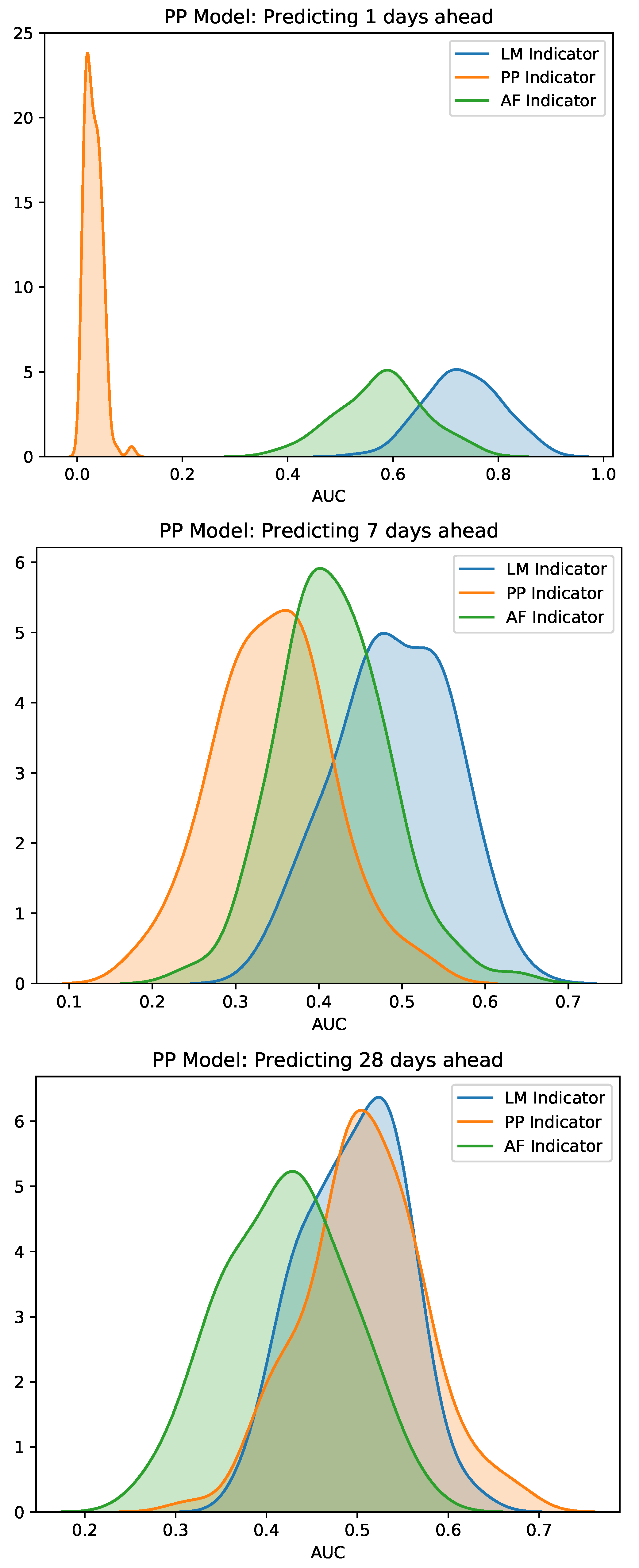
3.1. Early Warning Signals for Simulated Market Events

In this section we analyze the performance of the indicators for the various models, PP, LM and AF, introduced above. In all three cases we simulated the models for 50,000 time steps and recorded the last $16,000$ returns for further analysis, corresponding to roughly the number of trading days of the S&P 500 data. Each model was simulated 100 times. See Appendix A.2 for further details on these simulations.

For each series we have detected market events and then computed the ROC curve for the various indicators. To summarize our results, we in turn computed the corresponding AUC score. Figure 6 shows the distribution of AUC scores obtained over 100 simulation runs for return series generated according to the PP model. AUC scores are shown for predicting market events $d=1,7$ and 28 days into the future (from top to bottom). Especially when predicting over short horizons ($d=1$) the PP indicator works almost perfectly and, as expected, low indicator values precede market events giving rise to AUC scores close to zero. It appears that over larger horizons, none of the indicators is predictive with all AUC scores clustering around $0.5$.

Figure 7 shows the corresponding results on return time series simulated according to the LM model. In this case, all indicators seem to be of similar quality with none being perfect. Especially at larger time horizons there seems to be a slight edge for the LM indicator though. That the risk perception indicator derived from the AF model exhibits a similar performance could be somewhat expected as it, being a short term estimate of market volatility, also reacts quickly to raising volatility.

Figure 8 shows the corresponding results on return time series simulated according to the AF model. In this case, the AF indicator shows almost perfect performance with low indicator values, i.e., volatility, preceding market events. In contrast, the LM indicator looking for raising volatility is not useful reflecting that the mechanism of the model is completely different. Interestingly, the PP indicator is also predictive, but now with large indicator values preceding market events. The performance of all indicators drops just slightly when predicting across larger time horizons.

Overall, the indicators work reasonable well—mostly almost perfectly—with respect to the model they where designed for. In addition, on return series from other models they sometimes exhibit reasonable performance but can nevertheless be well separated as their behavior is sufficiently different across times series simulated from different models. We now turn to real market data.

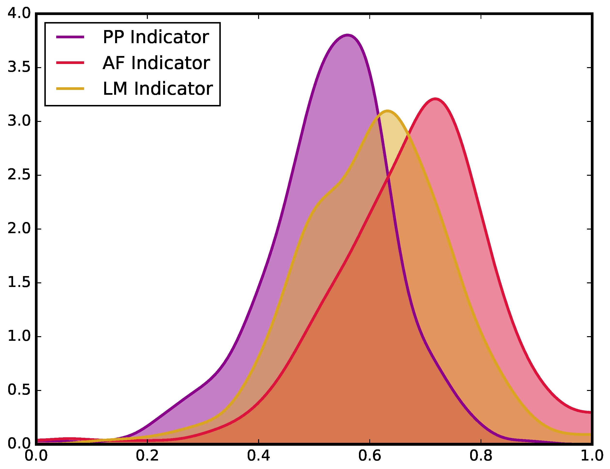
3.2. Early Warning Signals for Real Market Events

Here, we investigate the performance of all indicators on the return series from the S&P 500 between 4 January 1950 and 30 December 2016 as well as on stocks of the Forbes 500 universe. Based on availability, we selected 401 stocks for our experiments (see Appendix A.3).

Figure 9 shows the ROC curve of all indicators on the S&P 500 when predicting $1,7$ and 28 days ahead (from top to bottom). In each case, the grey areas show the 95% confidence region of ROC curves resulting from totally uninformative indicators. Thus, the performance of an indicator should be considered as statistically significant at the 5% level to the extend its ROC stays outside this region. According to this criterion, only the LM and AF indicators appear to be somewhat predictive for very short time horizon of a single trading day. Interestingly, in contrast to the results on the AF model, high values of the AF indicator are predictive. Thus, on the S&P 500 data, high or rising volatility indicate the onset of market events.

To further investigate the predictive performance, we have in turn tested the indicators on stocks of the Forbes 500 universe. Figure 10 shows the corresponding distribution of AUC scores obtained for one day ahead predictions. Whereas the PP indicators performs close to change level, on average over all stock tested, the other indicators shows some predictive power. Especially the AF indicator exhibits a very good performance in some cases, closely followed by the LM indicator. Note that the relative ranking of the indicators is most similar to the data simulated from the LM model. Nevertheless, the AF indicator appears somewhat better and the PP indicator is clearly worse with no tendency towards lower probabilities. In this respect, it appears that the structure of real market data is different than the model generated return series.

4. Conclusions

Starting from three econophysics models, each illustrating a different mechanism generating clustered volatility, we have derived early warning indicators for predicting the onset of turbulent market phases. In order to rigorously evaluate and compare all indicators, we have proposed a novel method for dating the onset of volatility clusters, i.e., market events. To this end, we fit a two-dimensional Hawkes process to tail returns and generate a market event if the intensity of the Hawkes process exhibits a large jump. Using simulated as well as real market data we have visually checked that this method produces market events that capture the intuitive notion of a volatility cluster reasonable well.

Next, we have introduced the ROC curve in order to systematically evaluated all indicators. These were then compared on simulated as well as real market data in terms of their AUC score. We found that the indicators are able to accurately predict market events on simulated data, especially on time series simulated from the model they were derived from. Furthermore, all indicators clearly distinguished between data simulated from the different models and achieved their best performance on data simulated from the same model they were derived from. Thus confirming our idea that different mechanisms could be detected based on specific statistical signatures. In contrast, the performance on actual market data is markedly lower and also more similar between the different models. Yet, over very short time horizons high or rising volatility appears to be able to predict market events to some extent, thus at least ruling out the mechanism based on low perceived risk. From this perspective, our findings confirm the results of Guttal et al. (2016) who found that financial crises appear to be preceded by increasing volatility. They have not investigated the problem of false alarms in a systematic fashion though. In this respect, our results substantiate their claims as the ROC curve precisely relates the ability to detect actual events with the rate of false alarms. Note that an informative signal, i.e., with a high AUC score, score would not be guaranteed to generate good trading returns, e.g., when used in an investment strategy. Yet, the idea to derive trading signals from agent-based models might be interesting to directly investigate in the future.

Overall, predicting the onset of market crashes—as attempted in this as well as other studies—remains elusive. We believe that substantial progress on this problem requires first and foremost a workable definition, ideally provided as an algorithm to allow large scale data screening, of what constitutes a market crash or event that is to be predicted. Modern machine learning has greatly advanced by relying on public data sets which allow for the systematic evaluation and compare different models. In particular, the price offered by Netflix in 2014 has prompted many other companies and academic institutions alike to open up challenging data sets to scientific research. With models becoming more and more complex, it becomes increasingly difficult to identify significant differences on purely empirical grounds. Thus, models need to be studied and evaluated from multiple angles and over multiple data sets. We believe that our contribution of indirectly testing model predictions in terms of indicators derived from instabilities, is valuable in this respect.

References

1. Adrian, Tobias, and Markus K. Brunnermeier. 2016. CoVaR. American Economic Review 106: 1705–41. [Google Scholar] [CrossRef]
2. Aymanns, Christoph, and J. Doyne Farmer. 2015. The dynamics of the leverage cycle. Journal of Economic Dynamics & Control 50: 155–79. [Google Scholar]
3. Bertschinger, Nils, and Iurii Mozzhorin. 2020. Bayesian estimation and likelihood-based comparison of agent-based volatility models. Journal of Economic Interaction and Coordination. [Google Scholar] [CrossRef]
4. Boettiger, Carl, and Alan Hastings. 2012. Quantifying limits to detection of early warning for critical transitions. Journal of the Royal Society Interface 9: 2527–39. [Google Scholar] [CrossRef] [PubMed] [Green Version]
5. Brownlees, Christian, and Robert Engle. 2017. SRISK: A conditional capital shortfall measure of systemic risk. The Review of Financial Studies 30: 48–79. [Google Scholar] [CrossRef]
6. Chakraborti, Anirban, Ioane Muni Toke, Marco Patriarca, and Frédéric Abergel. 2011. Econophysics review: I. empirical facts. Quantitative Finance 11: 991–1012. [Google Scholar] [CrossRef] [Green Version]
7. Chicago Board Options Exchange. 2019. The Cboe Volatility Index—VIX. Cboe White Papers. Available online: https://cdn.cboe.com/resources/vix/vixwhite.pdf (accessed on 20 November 2020).
8. Cont, Rama. 2001. Empirical properties of asset returns: Stylized facts and statistical issues. Quantitative Finance 1: 223–36. [Google Scholar] [CrossRef]
9. Diks, Cees, Cars Hommes, and Juanxi Wang. 2018. Critical slowing down as an early warning signal for financial crises? Empirical Economics 57: 1201–28. [Google Scholar] [CrossRef] [Green Version]
10. Drehmann, Mathias, and Mikael Juselius. 2013. Evaluating Early Warning Indicators of Banking Crises: Satisfying Policy Requirements. Technical Report 421. Basel: Bank for International Settlements. [Google Scholar]
11. Embrechts, Paul, Thomas Liniger, and Lu Lin. 2011. Multivariate hawkes processes: An application to financial data. Journal of Applied Probability 48: 367–78. [Google Scholar] [CrossRef] [Green Version]
12. Franke, Reiner, and Frank Westerhoff. 2012. Structural stochastic volatility in asset pricing dynamics: Estimation and model contest. Journal of Economic Dynamics and Control 36: 1193–211. [Google Scholar] [CrossRef] [Green Version]
13. Franke, Reiner, and Frank Westerhoff. 2016. Why a simple herding model may generate the stylized facts of daily returns: Explanation and estimation. Journal of Economic Interaction and Coordination 11: 1–34. [Google Scholar] [CrossRef] [Green Version]
14. Guttal, Vishwesha, Srinivas Raghavendra, Nikunj Goel, and Quentin Hoarau. 2016. Lack of critical slowing down suggests that financial meltdowns are not critical transitions, yet rising variability could signal systemic risk. PLoS ONE 11: e0144198. [Google Scholar] [CrossRef] [PubMed] [Green Version]
15. Hawkes, Alan G. 1971a. Point spectra of some mutually exciting point processes. Journal of the Royal Statistical Society Series B 33: 438–43. [Google Scholar] [CrossRef]
16. Hawkes, Alan G. 1971b. Spectra of some self-exciting and mutually exciting point processes. Biometrika 58: 83–90. [Google Scholar] [CrossRef]
17. Liniger, Thomas. 2009. Multivariate Hawkes Processes. Ph.D. thesis, ETH Zurich, Zürich, Switzerland. [Google Scholar]
18. Lux, Thomas. 2018. Estimation of agent-based models using sequential Monte Carlo methods. Journal of Economic Dynamics and Control 91: 391–408. [Google Scholar] [CrossRef] [Green Version]
19. Lux, Thomas, and Michele Marchesi. 1999. Scaling and criticality in a stochastic multi-agent model of financial market. Letters to Nature 397: 498–500. [Google Scholar] [CrossRef]
20. Lux, Thomas, and Michele Marchesi. 2000. Volatility clustering in financial markets: A microsimulation of interacting agents. International Journal of Theoretical and Applied Finance 3: 675–702. [Google Scholar] [CrossRef]
21. Meisel, Christian, Andreas Klaus, Christian Kuehn, and Dietmar Plenz. 2015. Critical slowing down governs the transition to neuron spiking. PLOS Computational Biology 11: e1004097. [Google Scholar] [CrossRef] [Green Version]
22. Ogata, Yosihiko. 1981. On Lewis’ simulation method for point processes. IEEE Transactions 27: 23–31. [Google Scholar] [CrossRef] [Green Version]
23. Patzelt, Felix, and Klaus Pawelzik. 2013. An inherent instability of efficient markets. Scientific Reports 3: 2787. [Google Scholar] [CrossRef]
24. Reinhart, Carmen M., and Kenneth S. Rogoff. 2009. This Time is Different: Eight Centuries of Financial Folly. Princeton: Princeton University Pressw. [Google Scholar]
25. Samanidou, Egle, Elmar Zschischang, Dietrich Stauffer, and Thomas Lux. 2007. Agent-based models of financial markets. Reports on Progress in Physics 70: 409. [Google Scholar] [CrossRef] [Green Version]
26. Scheffer, Marten, Jordi Bascompte, William A. Brock, Victor Brovkin, Stephen R. Carpenter, Vasilis Dakos, Hermann Held, Egbert H. van Nes, Max Rietkerk, and George Sugihara. 2009. Early-warning signals for critical transitions. Nature 461: 53–59. [Google Scholar] [CrossRef] [PubMed]
27. Scheffer, Marten, Stephen R. Carpenter, Timothy M. Lenton, Jordi Bascompte, William Brock, Vasilis Dakos, Johan van de Koppel, Ingrid A. van de Leemput, Simon A. Levin, Egbert H. van Nes, and et al. 2012. Anticipating critical transitions. Science 338: 344–48. [Google Scholar] [CrossRef] [PubMed] [Green Version]
28. Shiller, Robert J. 2005. Irrational Exuberance. Business and Economics. Princeton: Princeton University Press. [Google Scholar]
29. Stindl, Tom, and Feng Chen. 2019. Modeling extreme negative returns using marked renewal Hawkes processes. Extremes 22: 705–28. [Google Scholar] [CrossRef]
1.
In order to obtain volatility clustering, we had to increase β ten-fold compared to the original reference. This adjustment was stable across three independent implementations of the model in Python, Haskell and C++ which all produced identical results.
2.
Aymans & Farmer also discuss a policy rule for adapting α ( t ) . Since this does not substantially change the qualitative dynamics of the model we stick with α ( t ) α for simplicity.
3.
The bank’s equity at time t is given as E ( t ) = A ( t ) L ( t ) .
Figure 1. The S&P 500 return series along with the intensities of the Hawkes processes describing the 5 % quantiles of the positive and negative returns. The largest upward jumps of the Hawkes intensities are considered to mark onsets of market turmoil.
Jrfm 13 00301 g001
Figure 2. Return time series produced for purely endogenous information and the parameters in Equation (1) for 16 , 000 time steps. The red lines mark the times of market turmoil as detected by our method based on Hawkes process intensities.
Jrfm 13 00301 g002
Figure 3. Return time series in blue along with the ratio of chartists compared to the overall number of trading agents. One clearly sees that the volatility clusters if the ratio is close to one. As before, the red lines mark the times of market turmoil as detected by our method based on Hawkes process intensities. Interestingly, these correspond to local maxima of the chartist fraction even though this information was not available to the dating method.
Jrfm 13 00301 g003
Figure 4. Return time series generated from the leverage cycle model. Market crashes are clearly visible as strong negative returns and are reliably detected as market events (red) by our dating method.
Jrfm 13 00301 g004
Figure 5. Illustration of the receiver operator characteristic (ROC) curve: The left panel shows the distribution of indicator values which either where followed by an event or not. A warning signal is then raised if the indicator value exceeds a certain threshold. For each threshold, the fraction of correctly predicted events as well as the fraction of false alarms is recorded. Thereby, as shown in the right panel, the ROC curve is obtained. In the example, the indicator is informative with an AUC score of 0.89 .
Jrfm 13 00301 g005
Figure 6. A kernel density plot of the distribution of AUC scores for the various indicators on 100 return time series simulated according to the PP model. Results are for predicting events d = 1 , 7 and 28 days into the future (from top to bottom).
Jrfm 13 00301 g006
Figure 7. A kernel density plot of the distribution of AUC scores for the various indicators on 100 return time series simulated according to the LM model. Results are for predicting events d = 1 , 7 and 28 days into the future (from top to bottom).
Jrfm 13 00301 g007
Figure 8. A kernel density plot of the distribution of AUC scores for the various indicators on 100 return time series simulated according to the AF model. Results are for predicting events d = 1 , 7 and 28 days into the future (from top to bottom).
Jrfm 13 00301 g008
Figure 9. ROC curves for the different indicators for the S&P 500 time series when predicting 1 , 7 and 28 days ahead (from top to bottom). The grey areas show the 95% confidence region of ROC curves resulting from totally uninformative indicators. Thus, the performance of an indicator should be considered as statistically significant at the 5% level to the extent its ROC stays outside this region.
Jrfm 13 00301 g009
Figure 10. A kernel density plot of the histogram of areas beneath the ROC curves for the various indicators for return time series of all stocks in the Forbes 500 index.
Jrfm 13 00301 g010
Publisher’s Note: MDPI stays neutral with regard to jurisdictional claims in published maps and institutional affiliations.