Application of Genetic Algorithm to Optimal Income Taxation

Abstract

This paper, intended for researchers, introduces a stochastic method for calculating the optimal tax schedule based on taxpayer utility, population skill distribution, and wages. It implements and extends the classic approach to optimal income tax calculation introduced by J.A. Mirrlees. A genetic algorithm is applied instead of the numerical or analytical method of solving the problem. In the experimental part of the article, we took basic statistics for Germany in 2017 to infer about the distribution skills and wages of the working population. Their aim was to verify whether our approach would give similar results to those known from the literature on the subject. Thus, we have calculated the impact of the taxpayer attitude to work and budget external flows on the income tax schedule. Then, we measured the convergence of the search process across multiple runs of the algorithm. Analysis of obtained results brought us to the conclusion that they are similar to one known from the literature.

1. Introduction

In this paper, we describe results from transformation of a model of the income tax optimization to the statistical optimization framework based on genetic algorithms. We propose a method of a guided search of the solutions space, while the literature is dominated by a numerical or analytical approach. Our goal was to develop a more open and flexible framework for problem definition and finding the optimal solution through solutions space search. We were motivated by the fact that the stochastic optimization framework gives the researcher a more flexible and open method of defining the problem. This would allow modeling noncontinuous or even nonfunctional dependencies like some expressed by algorithms. Thus, it can be used for a better modeling of many real relationships difficult to denote and solve in the traditional way. This article describes an improved version of the model and algorithm introduced first in Małecka-Ziembińska (2012). The differences mainly lie in the technical improvements related to the optimization process.

However, the stochastic optimization has serious drawbacks as it does not guarantee finding the global optimum for the problem Ziembiński (2012). It may be particularly difficult for some highly-dimensional problems where the search space is particularly huge and the landscape of gradients embodied in it can be very complex. Thus, we believe that our contribution lies in the verification of the statistical optimization framework in the context of the optimal income taxation on some experimental data. For this purpose, we transformed and extended the model described in Mirrlees (1971) and conducted a series of experiments to evaluate the model. We wanted to verify if it delivers similar conclusions to one cited earlier in the literature.

The literature on subject of the tax optimization is rich and has a long history. The quantitative studies on the optimal taxation can be traced back to Ramsey (1927). However, while that paper discuses the optimal indirect taxes, it does not address income tax. Mathematical model of the optimal income taxation has been introduced in the paper Mirrlees (1971). The purpose of the tax optimization problem is to find the optimal income tax schedule that will maximize the social welfare. The paper describes the assumptions that led to the creation of a simplified economy model with a population of uniform taxpayers. First, it is assumed that the distribution of skills and associated wages is known in the population. Then, the same utility function describes the preferences of all taxpayers, and a single social welfare function determines the government’s tax policy. The paper contains a comprehensive solution to the problem obtained algebraically and numerically. However, results mainly have a theoretical impact because they were calculated for some arbitrary example configurations. Even so, the article explains many of the features of an optimal income tax schedule. Thus, the Mirrlees (1971) model appears to be a milestone in the research on the optimal income tax from the current perspective.

Some relationships that should be included in the simulated economy as proposed in Mirrlees (1971) had to be excluded due to complexity. They include differences in household size, preferences between taxpayer groups, the impact of tax concurrency between countries, migration, and social security, the impact of production and labor market structure. In most cases, they could not be easily introduced to the mathematical model due to their complexity for a realistically simulated economy. However, still, they may be crucial for the reliability and credibility of the result. It motivated us to search for another way for the problem definition and solution. We focused on stochastic optimization methods because they provide a conceptually open and flexible computational framework. From a rich world of different search methods, we chose a family of genetic algorithms. They are mature methods with properties and reliability thoroughly verified in recent decades. They also have a long history of successful applications in solving many technical and economic problems.

The problem definition introduced in Mirrlees (1971) has many assumptions. Some of them are simplifications required for the model solvability using contemporary methods. Because we refer to them in our model, they have to be enumerated in this paper:

• The consumption model defines only one type of labor and one commodity. The utility defines a concave function of consumption and leisure. Both goods are perceived by taxpayers as interchangeable.
• Taxpayers’ preferences are determined by the utility function, where the equivalent allocations of goods create indifference curves. Taxpayers are “homogeneous” because their preferences describe the same utility function. The government knows this taxpayers’ preference between consumption and leisure.
• A simulated economy takes into account a limited population of “homogeneous” taxpayers. Their distribution is described by the density function. Each taxpayer strives to achieve the optimal state determined by his utility function (e.g., individual’s egoism).
• Total utility for a population is the sum of individual utilities. However, aggregate utility is scaled nonlinearly to account for taxpayers’ reluctance to inequality. The scaling function determines the income tax schedule shape what defines its redistributive nature.
• Optimization covers a single period after which income tax is charged. Hence, the savings accumulated in the previous periods are ignored in the model.
• The model ignores the migration of people between countries. Thus, all effects of the tax competition between regions or nations are ignored too.
• Administrative and compliance costs are disregarded as their impact is considered negligible for the optimal income tax schedule.
• A “negative” income tax is considered and it is a subsidy paid from the budget to taxpayers.

The author found others environment features to be insignificant or having a marginal impact on the income tax schedule. As a consequence, it gave many simplifications and paved the way for the development of the solvable optimization model.

The model introduced in Mirrlees (1971) assumpes that the taxpayer’s population is described by the density function $f\left(n\right)$. Variable n denotes a range of skills and thus taxpayers can be distinguished on the basis of the skills assigned to them. The n’th skill reflects also a remuneration paid to the taxpayer for the performance of a unit of work.

The model defines the allocation of work to taxpayers with the work function $y\left(n\right)$. It is assumed that the work time values are marked in the range $\left[0;1\right]$. It leads us to the income before the taxation which is derived from the labor function according to formula $z\left(n\right)=y\left(n\right)·n$. The actual consumption of goods by taxpayers is calculated taking into account the income taxes collected or subsidies granted. If the tax charged is denoted as $t\left(n\right)$, then the taxpayers’ effective consumption is defined as $c\left(n\right)=z\left(n\right)-t\left(n\right)$.

The model is based on the assumption that there are two types of preferences in the optimized tax system. One, which affects taxpayers, is defined by the utility function $u\left(c\right(n),y(n\left)\right)$. This concave function is the same for all taxpayers. The other represents social policy and reflects an aversion to inequality. Thus, it captures the government’s redistribution policy, and it is defined by the $G\left(u\right)$ welfare function.

The income tax optimization problem introduced in Mirrlees (1971) centers on finding the $c\left(n\right)$ (distribution of consumption) that maximizes social welfare W, where, it is denoted as follows:

$$W={\int }_0^{\infty }G\left(u(c\left(n\right),y\left(n\right))\right)·f\left(n\right)\mathit{dn}.$$

(1)

It is worth noting that the $t\left(n\right)$ (tax schedule) is optimized indirectly by finding the optimal $c\left(n\right)$.

The findings delivered in Mirrlees (1971) suggest that the resulting optimal income tax schedule is close to linear. Obtained schedules often had negative income taxation (subsidies) for the lowest earning taxpayers. Moreover, the redistributive nature of the income tax was not obvious as only a slight reduction in inequality was observed after its imposition. The conclusion suggests that a hypothetical wage-based tax would be even more effective in improving social welfare. Many of these findings were challenged in later papers providing extended models, so it is necessary to mention at least some of them. It is particularly important because some conclusions will agree to results presented in our paper.

Extended concepts familiar to those described in Mirrlees (1971) were considered in Diamond and Mirrlees (1971). That paper presents research on the optimal taxation for direct and indirect taxes. It also discusses various tax practices in different countries. Subsequent studies on the income taxation were described in Atkinson and Stiglitz (1976). Their conclusions point to the need for taxes other than lump–sum taxes, which could result from the non-uniform characteristics of taxpayers. They noted that difficulties in observing taxpayers’ characteristics made it difficult to find the optimal income tax schedule. From our perspective, we believe that the statistical optimization framework gives us the opportunity to include such properties in the problem definition. Due to the fact that we can simulate the behavior of individual heterogeneous taxpayers instead of modeling them as a function of their skills.

Furthermore, Sadka (1976) suggests that some assumptions about finding a trade-off between equity and efficiency present in Mirrlees (1971) may lead to a confusing preference for a linear taxation. The author in Mirrlees (1971) verified findings from the perspective of max–min and utilitarian criteria. He found that the optimal income tax schedule is progressive for any utility function for which the elasticity of the substitution between leisure and consumption is equal to or less than one. On the other side, analysis in that paper concluded that, in some conditions, the tax may be regressive for higher income levels. Moreover, according to the author, it may be even fully regressive if the elasticity for substitution is greater than one and the predetermined level of public consumption is greater than zero. Thus, the degree of progression (or regression) depends strongly on the utility function shape and the scale of government needs. As we will show later in the article, the model we propose confirms some of these findings.

Another study described in Helpman and Sadka (1978) considers taxation of a full income. The full income is considered to be the taxpayer’s potential income. According to this study, the optimal average tax rate is progressive for the optimum conditions of Bentham and Rawl. However, marginal tax rates were progressive only to Rawl’s optimality condition. However, the tax does not have to be progressive if the earned income is taken into account alone instead of the full income.

A complementary analysis comparing different tax bases for the tax efficiency can be found in Blomquist (1981). Interestingly, the study used computational simulations to select the optimal tax base. The author assessed seven different tax bases using a computer program for gradient based nonlinear local optimization. The method uses a population of 500 virtual taxpayers in a simulated economy. In the conducted experiments, the CES utility function was used to determine taxpayers’ preferences. Authors assumed that the wages are exogenous what one may consider as unrealistic, thus they suggest research on endogenous ones too. However, under the above assumption, obtained results showed that the wage-based tax base is a promising alternative to earnings-based tax base. It offers the greatest gain of welfare. Hence, these findings Mirrlees (1971) confirmed conclusions.

On the other hand, a mixed tax system was examined in Stern (1984). The article describes optimal direct and indirect taxes and pursue the income tax research began in Stern (1976). It begins with a discussion of relationships between income and commodity taxes. It then proposes a combined taxation model supported by experiments done for the CES utility function at various elasticity. Acquired results were in line with the previous observations for income tax rates. Taxes grew with increasing aversion to inequality and decreasing elasticity of substitution in the optimal solution. Moreover, the demand to increase budget revenues progressed growth of income tax rates. It aligns with the previous findings.

More contemporary research on the optimal income taxation was described in Heathcote and Tsujiyama (2019). Authors provided an extensive research on various customization of the model introduced in Mirrlees (1971). They focused on relationships between model parameters and progressive or u-shape optimal tax rates. Delivered findings are similar to those from earlier studies. However, they found that distortions introduced by tax at low income levels may produce less pronounced growth of the marginal tax rate for these groups. They also found that u-shape tax rates are optimal when there are significant gains from high marginal tax rates at low income levels. Then, the subsidies are granted mainly to the poorest sacrificing the redistribution to the middle class taxpayers. It happens for high government expenditures (high predetermined level of public consumption) ending even at the regressive tax rates. It also happens if the planner has a strong taste for redistribution (e.g., higher preference to leisure).

Many other articles discuss the problem of the optimal income tax schedule. They introduce extensions related to taxpayers’ migration Mirrlees (1982), uncertainty of data known to governments Mirrlees (1990), diversified populations Kaplow (1996), Su and Judd (2006), Cremer et al. (2003), Kaplow (2008), and labor supply distortions Cahuc and Zylberberg (2008). These articles contain many interesting comments on some possible extensions of the optimal income tax model that could help better reflect real economies.

A method for optimizing personal income tax using a genetic algorithm was proposed in Morini and Pellegrino (2018). The authors optimize the personal income tax system with the example of Italy. They built a complex model of the Italian tax system and used a genetic algorithm to find the optimal values of the model parameters in the context of tax cuts reform. Their results suggest that there is a margin for improving equity in the Italian tax system. These studies were carried out further towards the application of multiple objective genetic algorithms Pellegrino et al. (2019). The authors noticed that the direction of tax reform may depend on conflicting criteria. Therefore, they propose multi-objective optimization for decision makers, which leads to a set of compromise solutions that form the Pareto front.

Technically, the result in our article comes from applying information technology research to the world of tax optimization. In particular, the optimization engine proposed in our contribution uses the genetic algorithm. It was developed to find the optimal income tax schedule in a very complex and highly dimensional space of possible solutions. The genetic algorithm is a stochastic optimization method that uses the concept of evolution to find the optimal solution. It monotonically produces better solutions in the following iterations, and it is relatively robust in avoiding local optima. Such robustness is an important feature because local optima are like “traps” for the stochastic search process. They can often occur in more complex problems and can prevent the search algorithm from finding the global optimum. This concept of stochastic optimization was proposed in Fraser (1957). He has evolved towards various fitness landscape search strategies. Some of them are inspired by nature—for example, the genetic algorithm Holland (1975). Historically, it was created on the basis of observations of evolution in the natural environment. The Goldberg (1989) book can be recommended to anyone who wants to learn more about the principles of this method.

2. Results

2.1. Main Contribution to the Optimal Income Tax Model

Our model proposed in this paper was built on the model introduced in Mirrlees (1971) with the contribution of the following new features:

• The amount of available labor in the simulated economy is limited. It is shared among the available jobs. The taxpayer’s earning ability is limited by his skill. Hence, each taxpayer is assigned a skill value. It limits taxpayers’ ability to find desired work as they can only get jobs that match or are below their skill level. It departs from the model defined in Mirrlees (1971).
• The value of the utility function depends on a consumption and a leisure. The income is calculated as the product of working time and wage rate, and the taxpayer’s consumption depends on his net income, taxes, and costs. However, the wage rate depends on the skills required for the assigned job. The leisure is calculated as the difference of the total time of life and working time. Moreover, in our framework, we can replace it with a complex utility calculation algorithm that takes into account various other inputs. Our approach extends a utility construction introduced in Mirrlees (1971).
• The optimized variables of this optimization model set up the redistribution curve. Thus, it is a list of income ranges and assigned values reflecting redistribution. Redistribution values are amounts of money taxed or awarded (for curve knots with negative values) to the taxpayer if his earnings fall within a specific income gap. The node-based structure of the redistribution curve does not depend on specific family of functions. Such approach helps to find even irregular tax schedules because each node of the curve contains an independently optimized variable. The number of dimensions in the solution search space is equal to the number of nodes in the redistribution curve. Hence, it is highly dimensional optimization problem and solution is not limited to predetermined family of functions. Such implementation differs from the model defined in Mirrlees (1971).

The approach proposed in Morini and Pellegrino (2018) differs from our proposal in various ways. We stick to the traditional model proposed in Mirrlees (1971). Therefore, our model includes homogeneous taxpayers described by their individual utility function and differentiated according to the value of skills. The value of skills limits a taxpayer’s ability to find better paid jobs and thus affects their earnings. In our case, we don’t use actual pre-tax income as the optimization parameter to get the result. Instead, we only use the population skills distribution to allocate jobs and the labor market structure inferred from input income data. Job allocation follows an optimized redistribution curve (solution dependent tax/subsidies), job limits (we consider limited labor demand). It maximizes the individual score of the utility function of each taxpayer in terms of income tax and job limits for a given skill. Thereafter, the pre-tax income is computed based on the job allocation data and the budget is determined to evaluate the solution. Hence, in our model, we inherently take into account the impact of the income tax system on the structure of taxpayers’ employment.

On the other hand, the model proposed in Morini and Pellegrino (2018) describes different parts of the population and distinguishes classes of taxpayers (e.g., married, single, self-employed). The authors introduced empirically driven parameterized model of the income tax system reflecting one implemented in Italy. Then, using the genetic algorithm, they search for the optimal values of the model parameters. Their fitness function was constructed to reduce loses of the taxpayers and keeping the budget revenues possibly intact.

From this perspective, our model seems to produce more general results, and it is less focused on the implementation of the specific income tax system. We provide a node based redistribution curve as a solution model that is able to detect non-trivial properties of the tax schedule that may arise when various new constraints, instabilities, shocks, or features are introduced. In our case, each node of the redistribution curve can change its value independently of the others. However, we have introduced a parameterized optional constraint that enforces some kind of fiscal simplicity, requiring a smooth redistribution curve in the output. It prevents the appearance of too exotic and impractical tax schedules in solutions.

The paper is intended for the community of research interested in applying stochastic optimization methods to the problem of optimal income taxation. The proposed definition of the problem does not take into consideration extensions like savings, optimization of the multi-cycle tax schedule, and many others. We focused on the transformation of the classical approach proposed in Mirrlees (1971) to the framework of the stochastic optimization.

As we will show, the obtained results reasonably illustrate the properties of the optimal income tax model. However, they should not be treated as direct advice to decision–makers. In our opinion, there is a complexity gap between micro-simulations and real macroeconomics. It is not always possible to isolate the process in the economy and consider it separately. However, often such isolate gives us valuable insight into the properties of the system under study. We hope that a more declarative model definition used in the stochastic optimization that we pursue here can help in the more complex model development.

2.2. Definition of the Computational Model

The labor market is simulated by a labor allocation matrix D. Columns m represent skills (jobs paid at increasing wages) and rows v represent a growing number of labor units. For each specific column and row of the labor allocation matrix $i\in 0,\dots ,v$ and $j\in 1,\dots ,m$, it is possible to define $w\left(j\right)$ as a wage for a unit of labor in j-th job and $l\left(i\right)$ a standardized quantity of labor associated with row i-th. The normalization bias of the labor time is labeled $l_{\mathit{top}}$ and the row at $i=0$ accumulates unemployment. Hence, the pretax income for the matrix cell can be calculated as $z(i,j)=w\left(j\right)·l\left(i\right)$. The number of skills, their associated wages, and the distribution of job quotas are the optimization parameters. The simulated population of taxpayers is labeled P. The k-th taxpayer $p_k\in P$ is allocated in the D at a particular cell coordinates denoted as $h_k=\langle i,j\rangle$.

The labor allocation for matrix D has some constraints. The model enforces taxpayers distribution according to limits in labor availability. The available work assignments are associated with the D columns. They are defined by the parameter $l_{\mathit{max}}\left(i\right)$, which limits the allocated (post–tax) labor supply for jobs requiring given skills.

The income tax is defined by the redistribution curve $R_d\left(g\right)$, where $g\in 1,\dots ,q$ and q is the number of income slots. The borders of income slots are defined by $R_b\left(g\right)$, where $R_b\left(0\right)=0.0$ and $R_b\left(q\right)=\infty$. The curve defines a positive or negative amount for each income slot. This amount is either a tax or a grant depending on whether $R_d\left(g\right)$ is positive or negative. Therefore, if $z_k$ is the pretax income of k-th taxpayer and $R_b(g-1)\le z_k<R_b\left(g\right)$, then $t_k=R_d\left(g\right)$ is taxed (or granted) amount. The income slots’ borders $R_b$ are optimization parameters while redistribution curve $R_d$ values are optimized variables.

The consumption of k-th taxpayer is calculated as $c_k=z_k-t_k-f_k(z_k,t_k)$, where $f_k$ defines some additional costs. The nature of costs described by $f_k$ may vary. The function may represent compliance costs of taxation, a tax free amount, allowances, or some other ”hidden” costs of taxation. Because $c_k$ cannot be negative in the optimization result; therefore, $t_k<z_k-f_k(z_k,t_k)$. This inequality imposes a constraint in the model on positive $R_d\left(g\right)$ values. Finally, the utility for k-th taxpayer is defined by $u_k(c_k,(l_{\mathit{top}}-l_k)/l_{\mathit{top}})$, where $l_k$ is labor for allocation $h_k$. Hence, if $h_k=\langle i,j\rangle$, then $l_k=l\left(i\right)$.

The labor allocation defined by $h_k=\langle i,j\rangle$ generates income $z_k$ of k-th taxpayer. The finding of $h_k$ for all $p_k\in P$ is generally nontrivial. Various strategies may be applied for this purpose. They may be implemented as the labor allocation algorithm resembling a particular real-life labor market. It is feasible in the stochastic optimization framework but difficult in the traditional problem solving approaches.

Calculations describing particular taxpayers’ budgets are propagated on the whole population P. Thus, the total tax collected from taxpayers T and total grants to taxpayers R are defined as follows:

$$T\left(P\right)=\sum _{p_k\in P}{t}_k:t_k>0,$$

(2)

$$R\left(P\right)=\sum _{p_k\in P}{t}_k:t_k<0.$$

(3)

Both sums are important for the budget equation in the simulated economy. However, in the stochastic simulations, it is difficult to ensure exact equality constraints. Applying them strictly would make the optimization process almost impossible because a number of feasible solutions in the search space would drastically reduce.

Therefore, it is proposed following inequality relaxing the budget constraint:

$$T\left(P\right)+B\ge R\left(P\right)+C_T\left(P\right)+C_R\left(P\right),$$

(4)

where B-money obtained or granted to the budget (they may represent transfers between the income tax system and some other fiscal components in the simulated economy), $C_T\left(P\right)$ is the tax administration costs, and $C_R\left(P\right)$ is social administration costs.

The inequality in the budget constraint should not be seen as conceptually troublesome. The algorithm minimizes the difference between both sides of the inequality accordingly to the problem’s optimization criterion. It happens because any excess of the money should be spared on grants for taxpayers or simply remain untaxed. Thus, any excess of $T\left(P\right)-R\left(P\right)$ would be naturally minimized during the optimization. The direction of the inequality was chosen according to the assumption that the collected taxes amount should be greater than the money spent. Thus, such budget in the acceptable solution is always feasible. Note that the budget inequality also puts constraints on negative values of the optimized curve $R_d$ representing subsidies.

The policy of the government is described by the social welfare function $G\left(u\right)$. This function represents the aversion to inequality in the population. It is a parameter of the optimization model assumed to be known by the government. This function is a crucial component of the optimization goal function, and it leads us to the following definition of the problem.

The problem of the optimal income tax schedule is finding a feasible $R_d$ values that would maximize the social welfare defined as follows:

$$\mathit{max}\sum _{p_k\in P}G\left(u_k(c_k,(l_{\mathit{top}}-l_k)/l_{\mathit{top}})\right).$$

(5)

The redistribution curve must be found for given: G, $u_k$, D, $l_{\mathit{max}}$, $l_{\mathit{top}}$, w, P, $R_b$, $f_k$, $u_k$, $C_T$, $C_R$, B, the labor allocation algorithm, and budget constraint.

It is worth remarking that the proposed computational model is an extensible structure that abstracts from a specific method of stochastic optimization. It can be easily extended to provide multi-cycle model for the optimal income taxation if we optimize a sequence of $R_d$ co-evolved curves. Such an extension would require separate labor assignments in subsequent cycles, and therefore be greedy for processing power.

2.3. The Model Customization

The model introduced above requires allocation algorithm, functions, and data as parameters to conduct experiments. We used the welfare and utility functions introduced in Mirrlees (1971) to retrieve comparable results. However, the proposed computational model can be easily reprogrammed with other functions if necessary.

Thus, the individual utility is defined as follows:

$$u(c,l)=\alpha ·log\left(c\right)+log(1-l),$$

(6)

where $\alpha$ is the scaling coefficient reflecting taxpayer’s preference on goods, c is the taxpayer consumption, and l is the taxpayer labor.

The social welfare function has the following notion:

$$G\left(u\right)=-\frac{1}{\beta }·e^{-\beta ·u(c,l)}$$

(7)

where $\beta$—the coefficient reflecting social aversion to inequality in the simulated economy, $u(c,l)$—the utility function. The default values in experiments were $\alpha =1$ and $\beta =1$. We used the social welfare as the negative function. It gets closer to 0.0 as individual utility increases. Such approach helps with reducing errors in aggregating social welfare when evaluating a solution. This is because its implementation on a positive exponential scale can give us a wide range of values that would add together causing numerical errors.

The labor allocation algorithm distributes the population in a real-market like manner. In our case, taxpayers in P with higher skills are allocated first. The allocation of taxpayers reduces the quantity of available labor which is delimited by $l_{\mathit{max}}\left(i\right)$. Therefore, if the available labor limit was exceeded for a given column of D, then the subsequent taxpayer is allocated to a lower paid but available quantity of labor. Thus, he is given an inferior job or sent to unemployment. This decision depends on the individual utility function $u_k$ value. It is calculated on the basis of the taxpayer location in the labor matrix D and redistribution curve R (through consumption and labor time). It should be maximized for the taxpayer within current labor availability constraints. Hence, the algorithm iterates through the matrix D cells seeking for the cell with available labor and maximizing $u_k$ (including cells reflecting unemployment). Subsequently, allocated taxpayers have lower skills and a lower probability of finding the job maximizing their utilities. Ultimately, some group of taxpayers with the lowest skills may remain unemployed. Thus, it is a kind of the best first allocation. It should reflect to some extent the real cases where more qualified taxpayers are sought to work than less qualified taxpayers. Hence, such highly qualified taxpayers have a privileged position when choosing to work in a competitive environment.

The above algorithm produces allocation $h_k=\langle i,j\rangle$ for all $p_k\in P$. It is computationally expensive and efficient for a few taxpayers (agents) used in the simulation. It relies on the utility calculation for each taxpayer for all cells in D at given redistribution curve $R_d$ and labor limits. Because calculated utilities are hardwired to $R_d$ and $u_k$, it appears that many of the calculations are redundant. Thus, in our implementation, a dedicated cache for intermediate calculations has significantly reduced computational costs of this algorithm.

The redistribution curve $R_d$ used in experiments comprised 40 nodes irregularly distributed. Nodes for lower incomes are located more closely to one another in this curve implementation. This is explained by the fact that most of the population falls into low or medium income slots. Thus, such nodes’ distribution makes the tax approximation more accurate for the range of low incomes. In the consequence, the redistribution curve border incomes $R_b$ are generated according to the following equation:

$$R_b\left(g\right)=-(1-\frac{1}{{\varphi }^{-(g+\kappa )}}),$$

(8)

where $\varphi >1.0$ is a parameter of the function determining the growing rate, $\kappa \ge 0$ is a parameter of the function determining the distribution shift. In the experiments, used settings were $\varphi =1.17$ and $\kappa =2$.

2.4. Experimental Data

A crucial part of experiments’ customization involves selection of data sets. Our model is proposed for observing the optimal properties of a tax schedule under different input settings, rather than for actual quantitative decision-making. Hence, we did not focus on exact data in experiments and used approximated ones. On the other hand, we would not like to use a fully artificial data set and break the connection to real-life. Thus, we focused on data set generated by “reverse engineering” from statistics on OECD.StatExtracts (2020) for Germany in 2017. In our opinion, such a set should correspond to a real case of a mature and stable economy. The one we need to verify properties of our Mirrlees model’s transformation.

According to Mirrlees (1971), the distribution of skills in the taxpayers’ population can be derived roughly from the distribution of income in the real balanced economy. Therefore, the term “skill” in the problem definition can be recognized more as the capability to earn money rather than some educational attainments. In our configuration, 50 levels of skills have been distinguished in the simulations.

In many countries, current data about taxpayers incomes are usually not published except for some general statistics. Hence, we “recovered” the distribution by an income curve approximation. For this purpose, we used statistics published in OECD.StatExtracts (2020) by using another genetic algorithm. Because it is not a main contribution in this paper and it is relatively trivial, we decided to not describe it here. However, some assumptions must be introduced to clarify data source.

The key issue in finding an approximation of the data is the selection of the appropriate income model. For this purpose, we use Lorenz curve $LC$ for cumulative share of people $p\in [0;1]$ ordered according to income (Lorenz 1905). A complex curve model proposed in Wang et al. (2011) was applied and denoted as follows:

$$\begin{array}{ccc}\hfill LC\left(p\right)& =& {\left({\delta }_{LC}·p+\left(1-{\delta }_{LC}\right)·L_{{\lambda }_{LC}}\left(p\right)\right)}^{{\alpha }_{LC}}\hfill \\ & & ·{\left({\delta }_{LC1}·\left(1-{\left(L_{{\lambda }_{LC1}}\left(1-p\right)\right)}^{{\beta }_{LC1}}\right)+\left(1-{\delta }_{LC1}\right)·L_{{\lambda }_{LC0}}\left(p\right)\right)}^{{\eta }_{LC}}\hfill \end{array}$$

(9)

Symbol p is a share of the taxpayer’s population. The following symbols ${\alpha }_{LC}\ge 0$, ${\beta }_{LC1}\in \left(0;1\right)$, ${\delta }_{LC}\in \left[0;1\right]$, ${\delta }_{LC1}\in \left[0;1\right]$, ${\eta }_{LC}\ge 0$, ${\lambda }_{LC}>0$, ${\lambda }_{LC0}\ne 0$, ${\lambda }_{LC1}\in \left(-\infty ;0\right)\cup \left(0;l{n}^{-1}\left({\beta }_{LC1}\right)\right)$ are model parameters, meeting conditions ${\alpha }_{LC}+{\eta }_{LC}\ge 1$ and ${\delta }_{LC}+{\delta }_{LC1}<1$. Furthermore, the equation:

$$L_{{\lambda }_{LC}}\left(p\right)=\frac{e^{{\lambda }_{LC}·p}-1}{e^{{\lambda }_{LC}}-1}$$

(10)

where ${\lambda }_{LC}\ne 0$ defines generic $LC$ model for the Pareto income distribution. A verification of $LC$ model applicability is described in Wang et al. (2011). Function argument p represents a cumulative share of people from lowest to highest incomes. According to the paper, the function provides the lowest error of approximation for data from the USA collected in 1983. Thus, it was chosen by us in our calculations to infer the income data approximation from basic statistics.

The goal optimization function for $LC$ approximation was parameterized with statistics available in OECD.StatExtracts (2020) for the Germany in 2017. We used the Germany data because we recognize it as mature and balanced economy in time well after 2008 crisis and before Covid. The goal function considers the income inequality (Gini coefficient Gini 1910) and poverty lines for the whole population before the taxation. The following values were taken $P_{\mathit{Gini}}=0.454$, $P_{\mathit{poverty}40\%}=0.28$, $P_{\mathit{poverty}50\%}=0.33$, $P_{\mathit{poverty}60\%}=0.36$. The poverty line in our case is the ratio of the population earning less than $40\%$, $50\%$, and $60\%$ of the median income. The curve optimization pass has delivered values for the parametrization of the model described by Equation (9). We denoted them in

Table 1. Lorenz curve parameters obtained for Equation (9) by the approximation.

${\mathit{\alpha }}_{\mathit{L}\mathit{C}}$	2.785002724509986	${\mathit{\lambda }}_{\mathit{L}\mathit{C}0}$	3.1358583948780385
${\beta }_{LC}$	0.11556036645313784	${\lambda }_{LC1}$	−0.0518184637825162
${\eta }_{LC}$	0.12814760297069056	${\sigma }_{LC}$	0.2531818236541253
${\lambda }_{LC}$	−0.8276942971333705	${\sigma }_{LC1}$	0.4111980827271129

. Found $LC$ well approximates published statistics. It offers the accuracy of two places after the decimal point for basic statistics took as parameters of the goal function.

The $LC$ results tell us about the distribution of income in the population, for example, if $LC\left(0.4\right)=0.2$, forty percent of the lower-income population earned a fifth of the total income. Obtained $LC$ was used for the generation of the income distribution curve used as input data required for experiments. The income distribution has been obtained from OECD.StatExtracts (2020) for the total income of $1.693037\times {10}^9$ (euro) and the total population of $43.2848$ millions of working taxpayers.

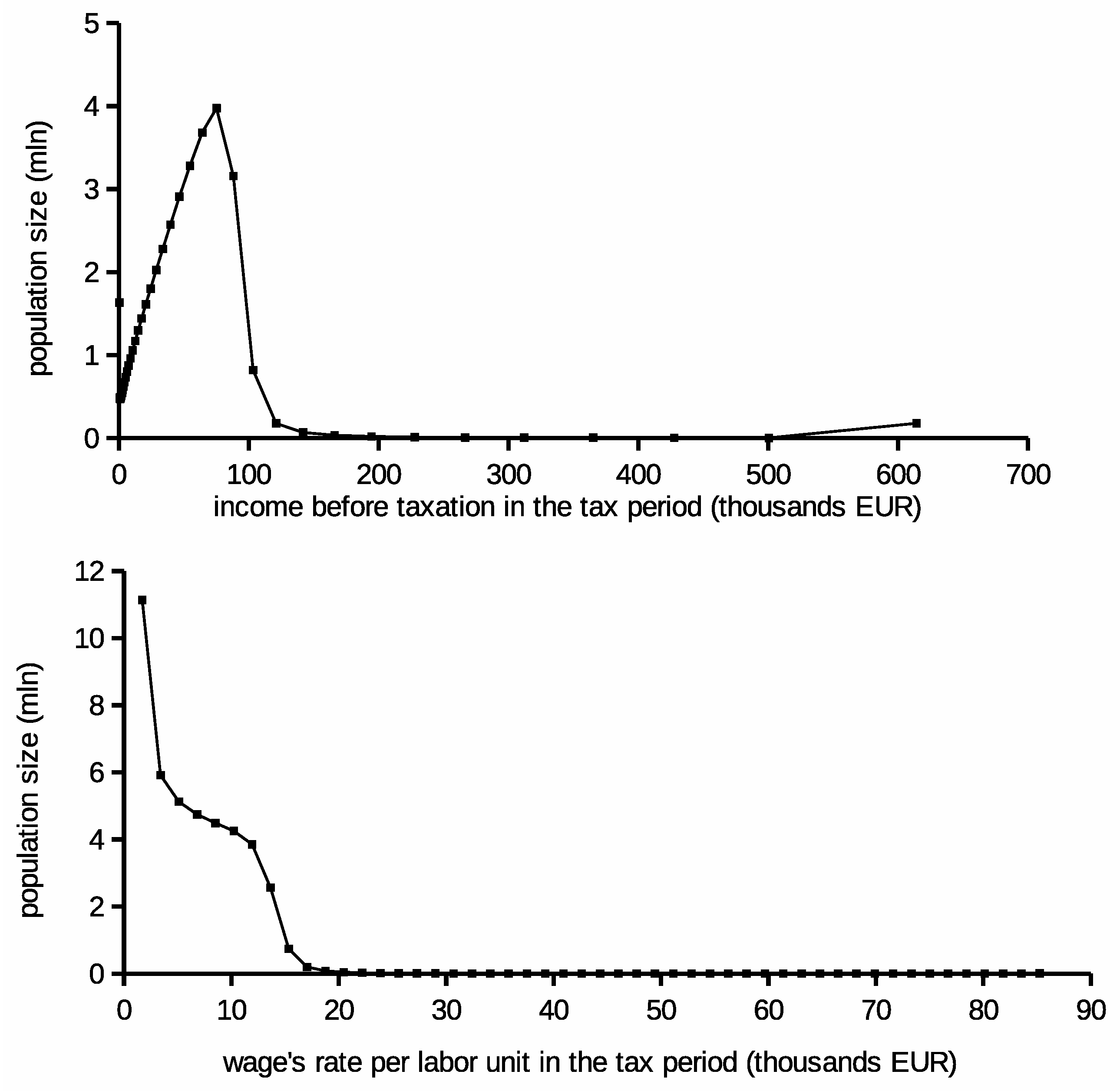
The pre-tax labor supply in the simulated economy was estimated from this population density distribution too. It reflects labor demand for balanced labor market (low unemployment). It is worth reminding readers that the $l_{\mathit{max}}\left(i\right)$ depends on skills (e.g., higher paid jobs are rarer in the economy). Approximation of $l_{\mathit{max}}\left(i\right)$ was done under assumption that each citizen works 6 h daily on average. This makes 1560 working hours for 260 days in a year and the total available labor of $6.75\times {10}^{10}$ work-hours. According to our model, each labor unit is allocated in the simulation to the whole tax cycle (e.g., year). Hence, each allocated labor unit in the simulation equals approximately 260 h in a year. The maximum allowed quantity of labor for taxpayer was set to $l_{\mathit{max}}=l_{\mathit{top}}=12$ units. The labor assignment has been done according to the allocation matrix that had 50 columns (skills) and 13 rows (labor).

The income and wage rate distributions are presented in Figure 1. The wage rate is shown per labor unit, which is equal to 260 work-hours. According to the model assumptions, taxpayers’ skills distribution depends on the wage rate. However, skills are uniformly scaled in the contrast to growing redistribution curve slots.

Calculation based on the whole population could be computationally expensive. In the context of stochastic optimization algorithms, where they are repeated multiply for each iteration almost impossible. Hence, the population was scaled down to 1000 representatives. Related $l_{\mathit{max}}\left(i\right)$ distribution was proportionally reduced to 6000 units. However, both scaling factors were remembered to provide the final result according the original values’ ranges be reverse scaling.

Furthermore, the distribution of the population has been tuned to ensure that at least three representatives are assigned to each skill. However, this modification disturbs slightly the distribution; it ensures that there is no discontinuity in the model setup. This is helpful in obtaining redistribution curves with more regular shapes. The reduction of the skills number or introduction of more representatives to the simulation are also possible as alternatives.

The following settings configure the budget equation and individual costs. A thoroughgoing presentation of all possible configurations would not be feasible in this paper. Therefore, for the sake of the simplicity, taxation and redistribution costs have been neglected in this description. It was assumed that $C_T=C_R=0$ and individual costs $f_k=0$. The default budget flow was neutral $B=0.0$.

2.5. Evaluation

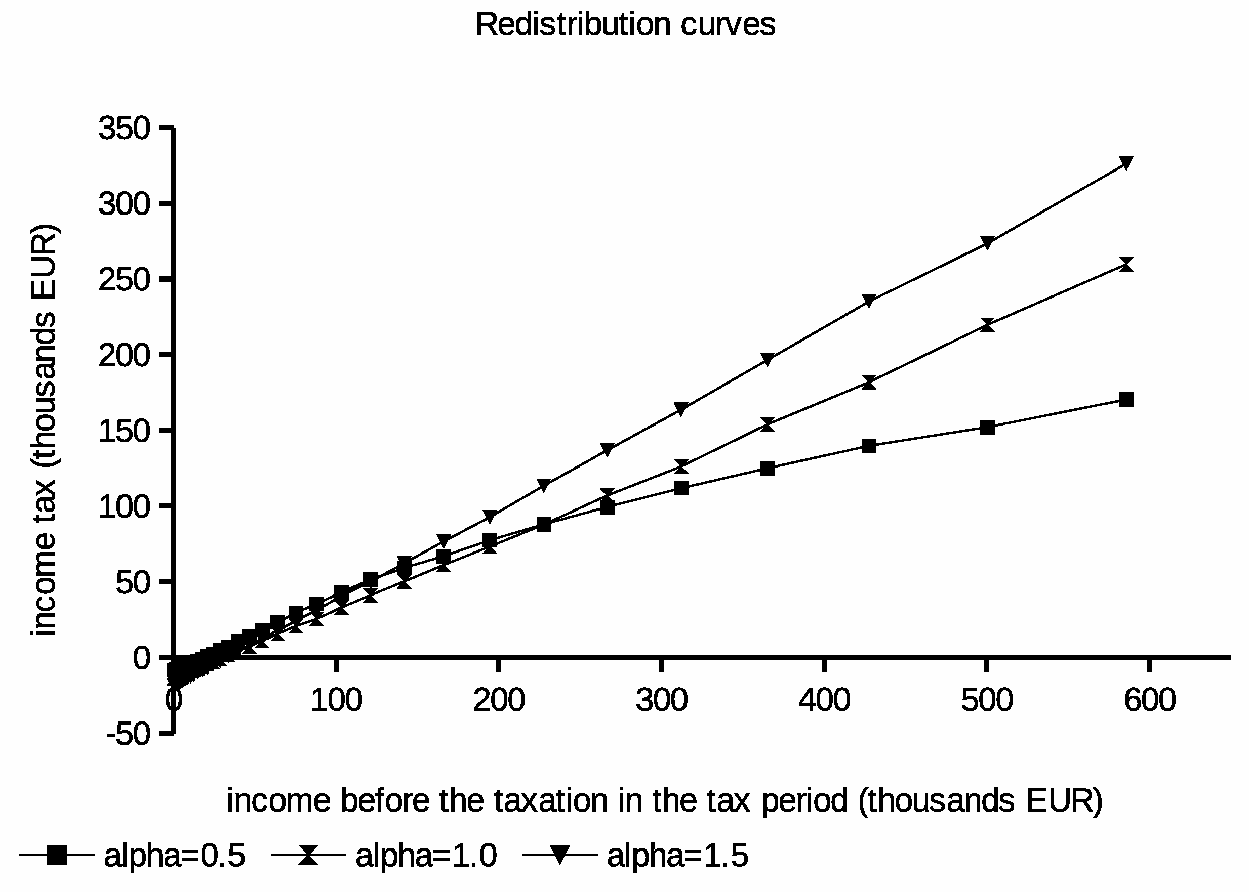
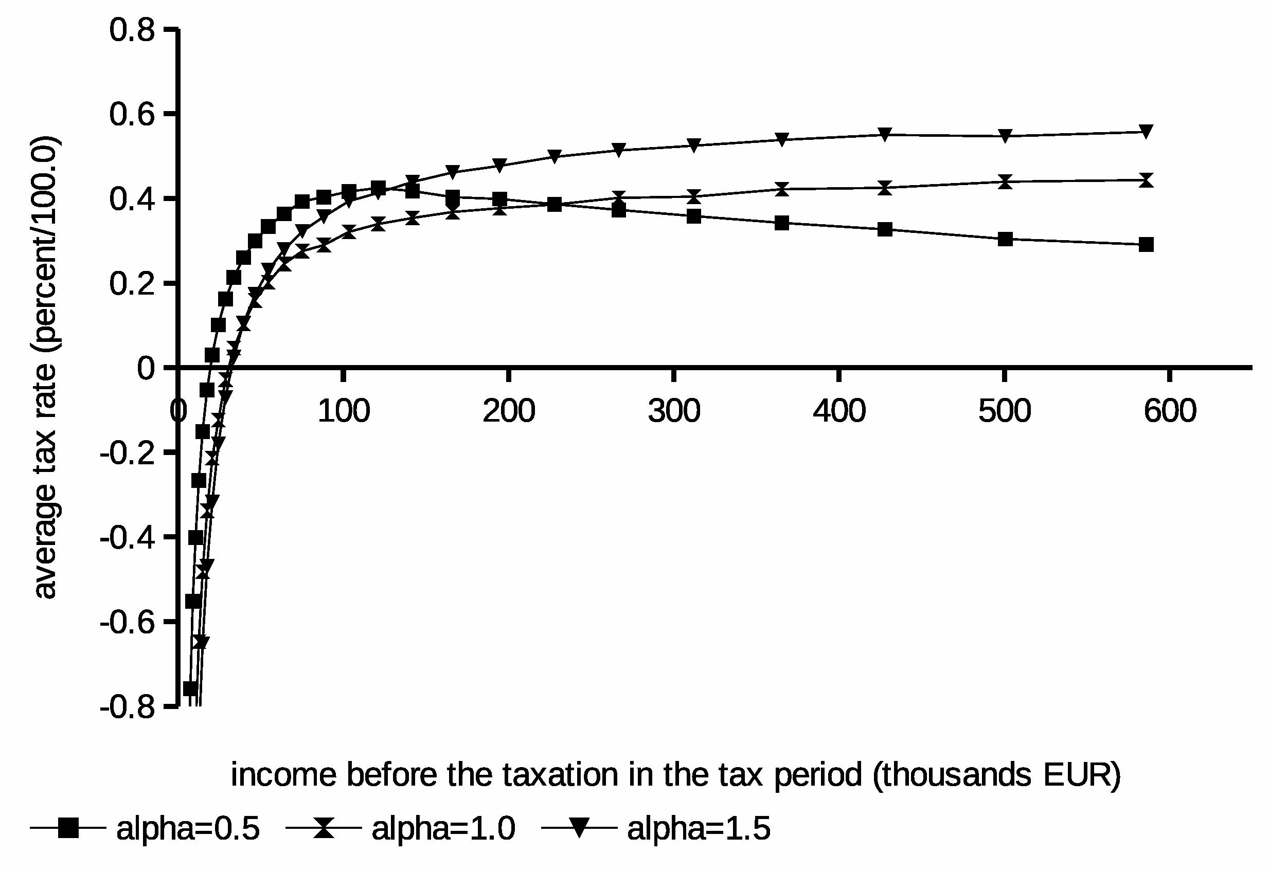
The initial set of experiments has been conducted for three different $\alpha$ values for the individual utility function.

They represent different taxpayers’ preferences between consumption and leisure, which has a significant impact on taxpayers’ labor supply. Redistribution curves obtained as solutions from optimization are plotted in Figure 2. Moreover, the derived average tax schedules obtained from these curves are in Figure 3. Statistics from produced solutions are summarized in

Table 2. Results from simulations for different $\alpha$ values.

Parameter Value ($\mathit{\alpha }$)	0.50	1.00	1.50
The social welfare value before the taxation and the redistribution	−10.50	−77.90	−577.70
The social welfare value after the taxation and the redistribution	−7.93	−38.97	−172.26
Total income produced (millions EUR)	792,862.3	1,247,232	1,319,852
Total collected income tax (millions EUR)	201,446.2	287,157.8	389,690.3
Total redistributed money (millions EUR)	201,446.2	287,157.8	389,690.3
Budget balance (thousands EUR)	10.72	24.06	39.48

.

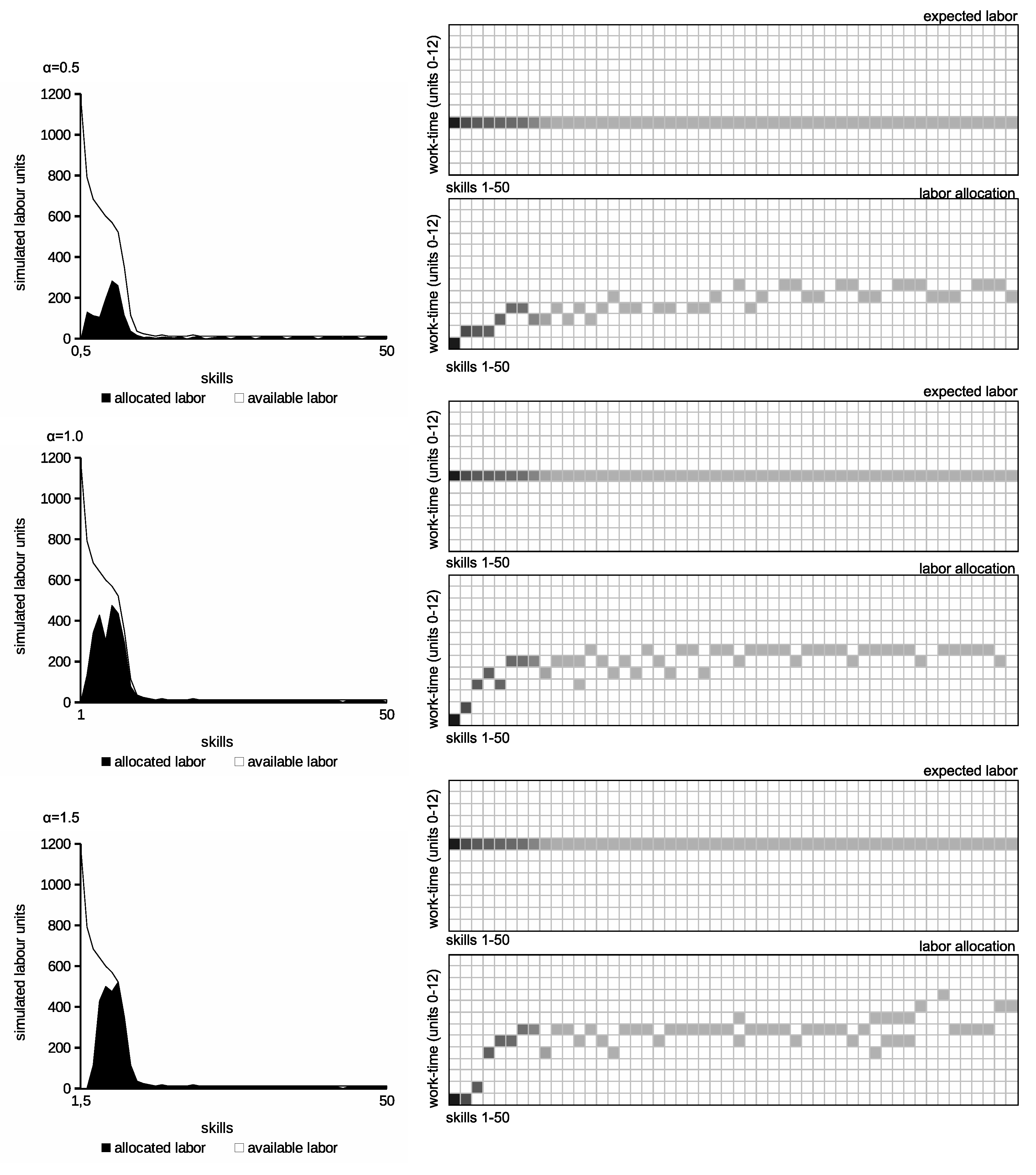
Results obtained from these experiments show that the lower $\alpha$ values lead to the observable increase of the income tax for low and medium earners. For the same schedules, the tax may drop for high earners. This result can be explained by an increased positive attitude for the leisure resulting from the low $\alpha$ value. Such labor–leisure preference results in the lower labor assigned to the population and lower produced income. In the consequence, taxes imposed on low earning taxpayers are higher. This interpretation is confirmed by results describing labor allocation in Figure 4. These charts show available and allocated labor distributions according to skill levels. Thus, they represent the distribution of labor demand and supply after tax. The grids in the right-hand column show the distribution of taxpayers in the D matrices for the various $\alpha$, where the darker boxes represent the denser population assigned to the matrix cell. They show the “labor allocation” computed by the algorithm considering $u\left(k\right)$ and $l_{\mathit{max}}\left(i\right)$ limits. On the other hand, the “expected labor” grids show the taxpayer’s ideal allocation in D according to individual $u\left(k\right)$ in the absence of income tax and $l_{\mathit{max}}\left(i\right)$ limits. The figures suggest that low $\alpha$ values cause unemployment in low earning taxpayers. It must be balanced by higher taxes imposed on the working population. The labor allocation figures show some dispersion for some high earning taxpayers. This is caused by small $l_{\mathit{max}}\left(i\right)$ for high earning taxpayers. Thus, it should be understood as a kind of artifact of the discrete nature of the presented model.

Interestingly, for the low $\alpha$ value, the redistribution curve observably depends on the income’s distribution in the population. This could lead to u-shaped schedules where the most tax burden is imposed on medium earning taxpayers. The unemployment is reduced for $\alpha =1.5$, but the average taxes imposed on the higher earning population are the highest. In this case, the positive attitude for the work causes even higher taxes for high earners to not cause an observable decrease of the utility for them. In conclusion, results from initial experiments explain that the balance between redistribution and taxes clearly depends on the positive attitude of the society toward the work. They also indicate that barriers in getting suitable jobs by taxpayers e.g., institutional, procedural, or juridical may lead to lower taxes and a higher need for the redistribution leading to worse budget performance.

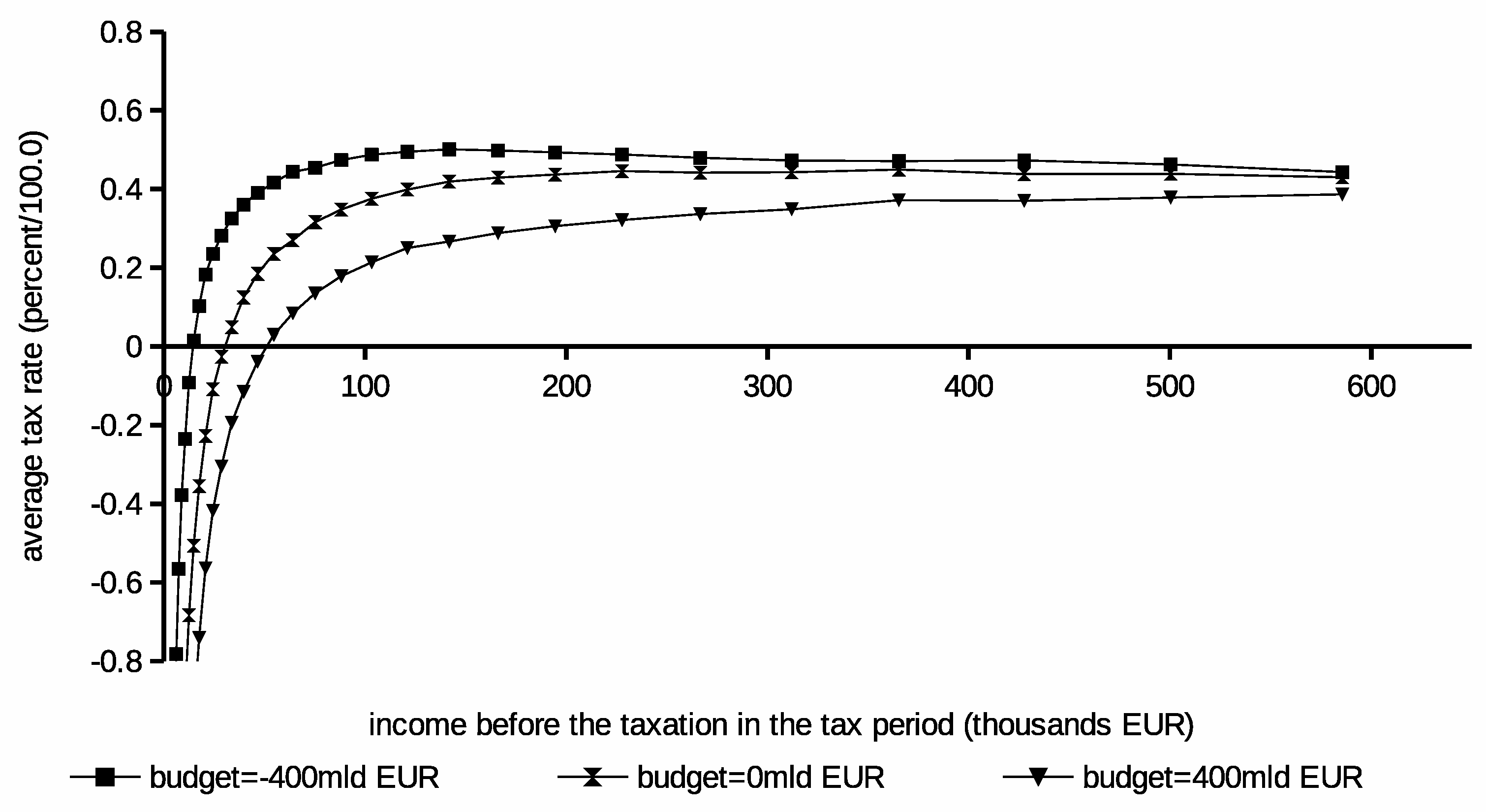
The second experiment was conducted to reveal the impact of budget flows on the income tax schedule. Three different B settings were considered. The optimization pass produced results shown in Figure 5. Solutions’ budgets are summarized in

Table 3. Simulation results for different B values (budget flow).

Parameter Value (Budget Flow B)	−400,000,000	0	400,000,000
The social welfare value before the taxation and the redistribution	−77.90	−77.90	−77.90
The social welfare value after the taxation and the redistribution	−58.95	−39.02	−28.06
Total income produced (millions EUR)	1,315,282.0	1,179,599.0	1,107,163.0
Total collected income tax (millions EUR)	522,595.7	310,216.0	189,271.2
Total redistributed money (millions EUR)	122,595.7	310,193.6	589,271.2
Budget balance (thousands EUR)	9.23	22,412.9	2.03

. The plots show gradual growth of the tax burden if the outflow of money from collected taxes (e.g., for other purposes than redistribution) is increasing. Moreover, the social grants are decreasing noticeably at the same time. This experiment’s results lead to the conclusion that e.g., public debt’s cost or other expenditures has a profound impact on the income tax schedule. The outflow increase leads to reduction in social welfare due to higher taxes and lower social grants. The burden related to this negative “offset” propagates on all income groups in the population. Thus, it clearly lowers the income level at which taxpayers stop receiving the social contribution and start pay the income tax. Both experiments were run in our engine for 4,000,000 iterations.

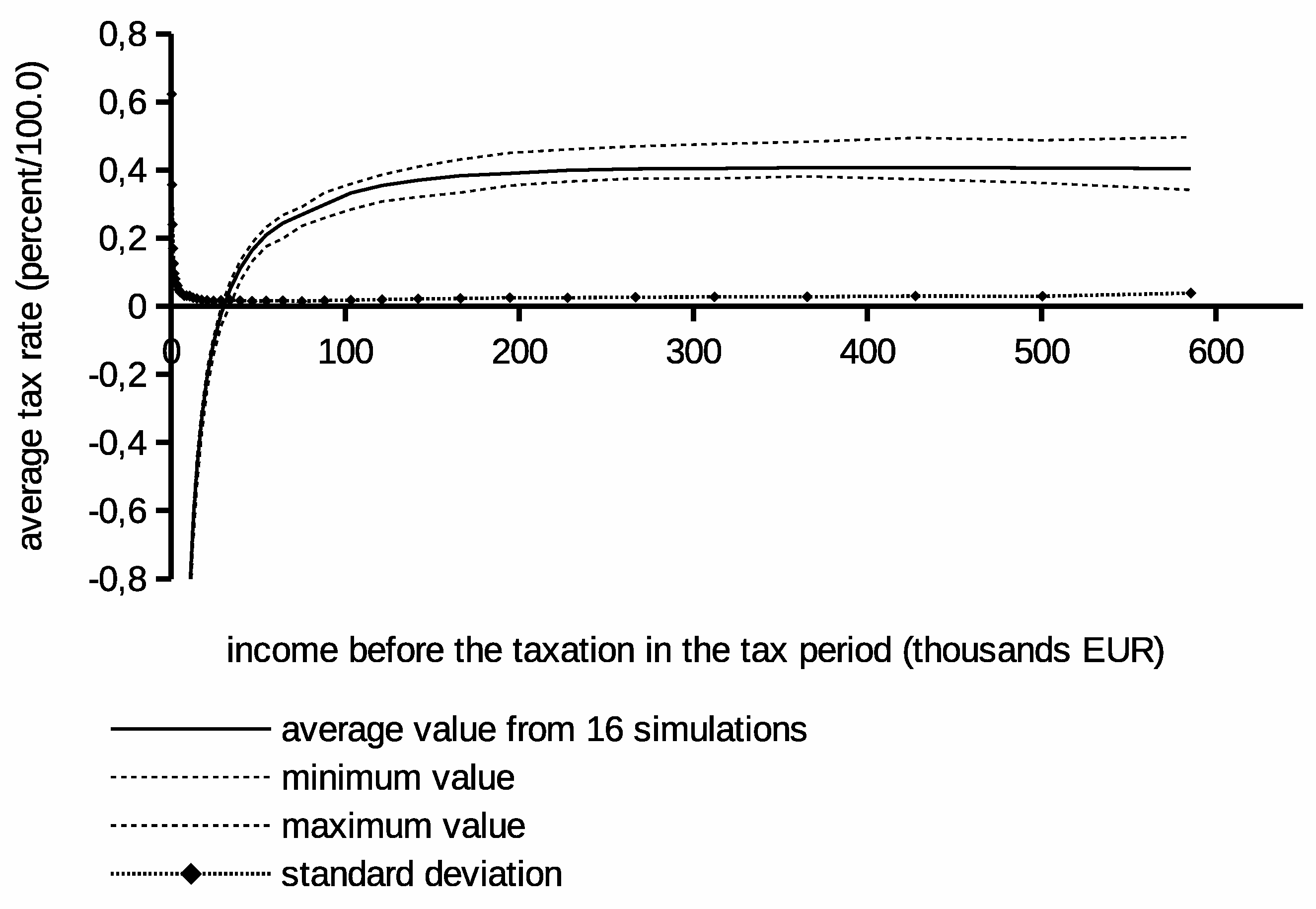
The last experiment has verified the stability of the proposed optimization method. In this experiment, the same calculations have been repeated 16 times with different initial pseudo-random generator settings. They were run for the same number of iterations equal to 3,000,000. It should produce comparably optimized solutions. It is known that the quality of the result depends monotonically on the number of iterations in the stochastic optimization. Therefore, we wanted to observe if results converge. The range of tax values confining all obtained tax schedules is plotted in Figure 6. Corresponding statistics describing the resulting budgets are in

Table 4. Aggregates obtained from repeated simulations.

	Values
	of the Best Solution	Average	Minimum	Maximum
The social welfare value after the taxation and the redistribution	−38.61	−39.01	−39.47	−38.61
Total income produced (millions EUR)	1,254,896	1,227,233	1,107,394	1,300,785
Total collected income tax (millions EUR)	289,811	294,402	257,932	332,073
Total redistributed money (millions EUR)	289,810	294,400	257,931	332,073
Budget balance (thousands EUR)	1097.50	1626.29	1.75	14,350.18

. We can observe that all solutions fall within a relatively narrow range of values after a few iterations. Note that the average values from all simulations in Figure 6 are not a tax schedule. It only tells about the position of the average of the 16 individual proper solutions.

If our method would deliver in repeated simulations strongly different results, then the divergence could thwart credibility and applicability of computed results. In our case, most of the simulation runs deliver results that converge. The observed dispersion is probably due to an insufficiently optimized budget inequality in some individual cases. Obviously, an optimization involving a larger number of iterations could result in tighter convergence of solutions, and the range band in Figure 6 might be narrower. However, the stochastic optimization method does not guarantee that (local optima).

3. Discussion

The described model does not take into account many circumstances in the real economy, such as the impact of other taxes. Therefore, the results presented should not be taken as direct guidelines for policy-making in the real economy without further research. However, they may help you identify relationships in tax schedules that arose from different settings used in experiments. An expanded model considering complexity of the whole tax system, interactions with other components of the economy, labor, and financial markets may be required to deduct policy-making ready guidelines. It is necessary to fill it with accurate real–life data.

Nevertheless, the results of the $alpha$ and B experiments appear to be comparable to ones described in Sadka (1976) and Heathcote and Tsujiyama (2019). In both articles, it was stated that the attitude to work and external budget flows have a profound effect on the optimal tax rate. Particularly, aversion to work or high budget expenditures produce u-shaped schedules. Our results acknowledged these findings. We found that changing the income tax schedule has a significant impact on the labor market. As a consequence, it has an observable impact on the total amount of wealth produced in the economy.

The proposed labor allocation algorithm is just an example of many possible ones. In an extended model, each kind of job may require a customized algorithm corresponding to behavior of the particular real-life labor market. Moreover, the labor allocations and the redistribution curve can be optimized together in the more flexible optimization configuration. It would vastly increase the number of search space dimensions. In such an alternate configuration, taxpayers may migrate between adjacent cells of the labor allocation matrix during optimization to maximize their utility. Such approach could further increase the social welfare in the simulated economy. However, the resulting labor allocation would not fit the case of a free market—primarily because it is necessary to “altruistically” divide labor between taxpayers, which in practice would require a significant control of the labor market by the government.

Furthermore, repeated experiments in the stochastic framework for the same configuration can deliver interesting knowledge about the simulated economy properties. Various suboptimal results obtained for the same number of iterations reflect the landscape of solutions in space. Such pool of solutions for slightly different values of the goal function usually covers a niche around the optimum in the explored search space. In our case, they have slightly different social welfare values. They can indicate which parts of the redistribution curve are more prone to modifications and which ones are more hardwired to optimization parameters. A set of similar schedules, scattered around the optimal, can be used to identify income groups for which the income tax schedule may change with little negative impact on the social welfare of the entire population. In this way, repeated simulations can be used as a tool to analyze the sensitivity (or elasticity) of the income tax schedule.

From the computational point of view, our choice of the genetic algorithm to solve the problem of optimal income taxation was motivated by the following considerations:

• A problem for the stochastic optimization method can be formulated more declaratively. This formulation may involve complex nontrivial relationships in the simulated economy. These features may be defined in nonlinear equations and for nonmonotonic or noncontinuous functions or even by algorithms. Hence, it is relatively easy to add some features e.g., groups of taxpayers, households differences, allowances, administrative expenses, compliance costs, execution, international tax competition, relationship to some other taxes, and regional differences between taxes. Additionally, nontrivial constraints on the tax schedule may be easier imposed on the solution.
• A flexible modeling framework can be useful in the processing of data collected in real economies. This method makes it possible to model significant parts of the real economy and study their behavior in simulations. Thus, it allows for ”what–if” analyses that may be used to assess effects before proposed changes to the tax system are introduced to a real economy.
• The proposed computation method is relatively easy to scale. Thus, the power of the modern computing clouds can be utilized to find the solution fast. The method allows for iterative refinement of the obtained solution to the acceptable level of ”quality” under the feasibility constraints. Moreover, it is possible to begin the optimization from a simple tax schedule and gradually evolve the solution towards a more complex one with the better score.
• The genetic algorithm produces better solutions by modifying the current population with use of operators. These operators are often derived from observations of evolution in biology e.g., mutation, cross-over. They produce child solutions and, after that, the algorithm selects those of them which benefit the population. However, certain domain-related operators can also be used in the optimization. They would utilize the knowledge of properties of the optimized problem. Despite the fact that they may reduce the universality of the genetic algorithm implementation, their introduction may greatly improve the efficiency of computations for the particular optimization problem. Moreover, they can be very useful in later stages of the optimization where near-optimal solutions require more precise adjustments to produce the offspring. In the problem of the optimal income taxation, they may modify the income tax schedule according to the population density or the labor supply.

In addition to genetic algorithms, many other alternative stochastic optimization methods have emerged in recent decades. They include extensions to Monte Carlo method, the tabu search, the simulated annealing, and various particle swarm optimization methods. Clearly, they can be considered as alternatives to the optimization problem under study. They have different computational properties due to different search space exploration techniques, which in some cases may lead to better results. However, according to the no–free lunch theorem, known from evolutionary optimization, any method could dominate the others for all possible optimization problems.

Despite the many advantages of the proposed optimization method, some limitations should be mentioned to get a complete picture:

• In general, the stochastic method does not guarantee the delivery of an optimal solution. Rather, it allows for gradual improvement of the population of solutions. Moreover, it is not possible to determine whether the produced solution is actually globally optimal. Additionally, many optimal solutions may coexist with the same evaluation scores. Unfortunately, the proposed method is incapable of determining and delivering all of them.
• Better solutions are generated by applying modifications to optimized values by various operators. The method browses for solution to the search space. It causes that the mathematical proof for the solution cannot be easily provided. We only know if it is feasible and the score of the goal function. Thus, the properties of the obtained solution can only be studied behaviorally. Therefore, it is difficult to trace the relationship between the parameters of the problem definition and the obtained solution.
• The genetic algorithm requires an initial population of feasible solutions to start the optimization. Generating such a set is in some cases non-trivial and strongly affects the results for discontinuous search spaces. Numerous strong constraints in the definition of the problem may cause fragmentation of the feasibility regions of the search space.

Due to the above features, genetic algorithms may deliver some nontrivial solutions for non–trivial problems. However, they would not provide the formal explanation of the produced solution. Thus, the proposed method is not a silver bullet. In our opinion, the reason behind applying a stochastic method to find the optimal income tax schedule lies mainly in the expandability of the proposed method.

4. Materials and Methods

Architecture of a Genetic Algorithm

We have implemented complex genetic algorithms as a solution space search tool because our optimization problem is highly dimensional. In our case, we optimize each node of the redistribution curve independently. Thus, the curve defined with 40 nodes is searched for in a 40-dimensional search space. The landscape of the fitness function is non-trivial as we evaluate the labor market through discrete job allocation, which is a combinatorial task. Combinatorial tasks are especially difficult with stochastic optimization methods because the fitness function has sudden and frequent changes with little or no smooth gradient. This makes them difficult to explore for population based stochastic algorithms. 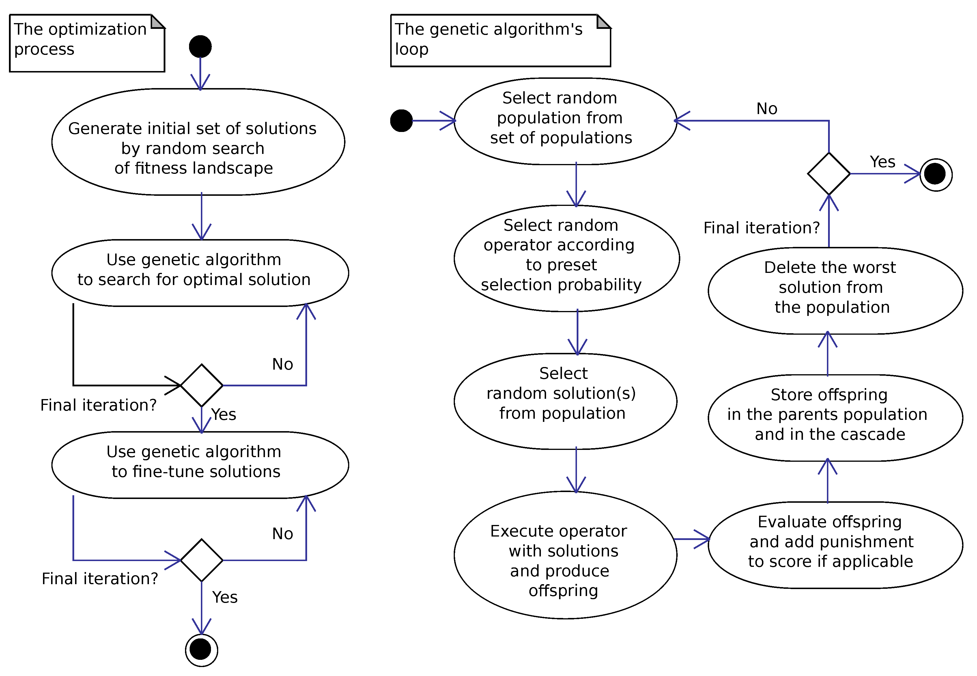To solve this problem, we preceded the search of the genetic algorithm by an intense randomized examination of the solution space as presented in Figure 7. Then, the genetic algorithm starts working. Initially, we optimize the curve by loosening the constraints. Such an approach causes the subspace of feasible solutions to be larger, and the algorithm cannot get stuck in a subspace of the fitness landscape cut off by constraints. Then, we fine-tune the solutions using the genetic algorithm and the required narrow constraints.

The genetic algorithm has a straightforward design that is explained in Figure 7. Like in other algorithms of its kind, it maintains an ordered population of solutions. It randomly selects a subset from them and constructs a new offspring solution using the operator. A child undergoes the evaluation and is moved to the main population on the position relevant to the score. The evaluation relies on the goal function (the objective function) which reflects the optimization criterion. The algorithm maintains a stable-sized population and removes the worst solution from the population if one better emerges. Thus, it ensures the convergence of the entire population to the optimum (most often local one).

The population-based search allows the algorithm to explore efficiently the space for better solutions. We can imagine that the solutions from the population are scattered over the curves of the search space carved by the objective function. The population scattering allows the genetic operators to produce better offspring and avoid local optima. Some operators may use the domain knowledge to create fitter offspring. They are less likely to construct an infeasible solution due to unmet constraints. However, more sophisticated operators lack generality and are only effective in the later optimization stages to fine-tune the final set of solutions.

While theoretically the basic genetic algorithm can solve any optimization problem, its architecture is often tweaked to improve its performance. The generic algorithm can be inefficient in a highly multidimensional search space. However, the improvement can be obtained by maintaining a set of sub-populations that are evolved in isolation. Such approach was used in our implementation. It allows for avoiding some local optima and performing the optimization for more complex problems. It also allows for scale–up processing because the computations can be distributed among many computers at the same time. Efficiency can be further improved by choice of appropriate solutions for the reproduction. They should not be too similar because then they could converge too quickly to the local optimum, or be too different because they could produce an infeasible or unfit offspring.

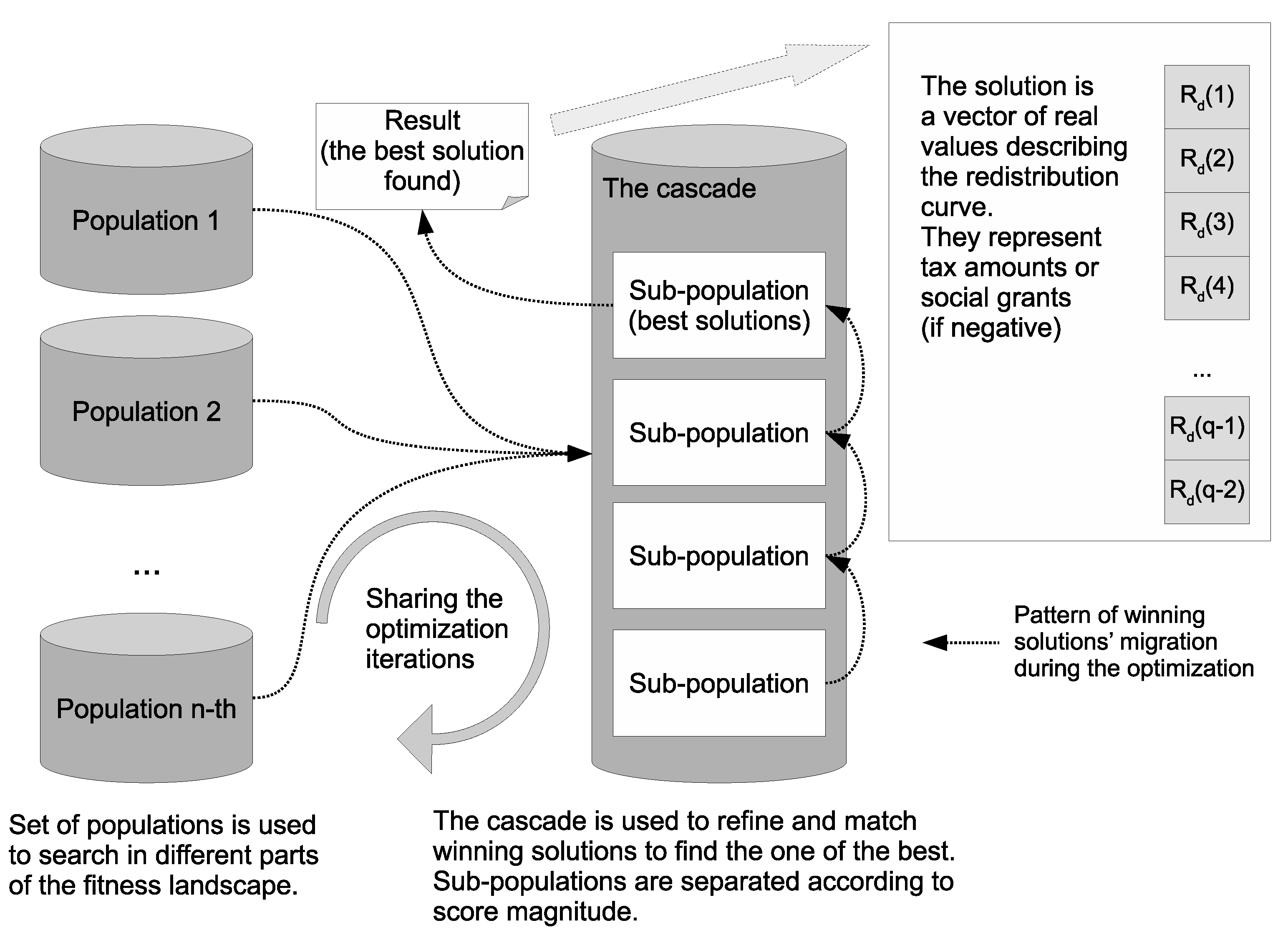
According to above remarks, the algorithm implemented in our research maintains a set of 24 sub-populations arranged according to Figure 8. These sub-populations share algorithms iterations but independently converge in the search space. Moreover, under certain circumstances, a migration of solutions is possible between these sub-populations. In our implementation, a parallel cascade of sub-populations ordered according to goal function score is also implemented. Such architecture allows for conducting the optimization within a given ”quality” class of solutions. The top sub-population of the cascade contains the best solution from all received during the optimization. The following sub-populations contain solutions with scores worse by the magnitude. The cascade prevents the mixing of poor and good solutions during offspring generation as parents have to come from the same sub-population. Crossover of different solutions often produces solution with the score worse than the worst from parents. It may even produce an infeasible solution. As a result, many iterations can be wasted creating low-quality solutions. The separation brings more accurate selection of parents for the reproduction and the better convergence. Of course, the exchange in the cascade populations also occurs as offspring can migrate up it according to individual score. In this way, the overall quality of the population in the cascade can be improved during the optimization. The cascade could be replaced by a single population of winners from sub-populations, but, as such, it would converge slower. In our case, the cascade had four sub-populations.

Operators contain crucial tools for the optimization performance. Fortunately, the optimization problem under consideration has many properties that allow us to construct some dedicated operators The algorithm optimizes the redistribution curve containing a sequence of nodes which determine taxed or granted subsidies. Generally, each value in a curve node should be a threat as an independently optimized variable. However, due to the characteristics of the underlying labor market, the optimized variables are interdependent. Moreover, it is known that highly irregular tax schedules would be costly and difficult to explain for taxpayers in real life. Therefore, as such, they should be considered as infeasible solutions. A received feasible solution should contain a rather smooth transition of taxed amounts along increasing incomes. Ultimately, the obtained result should match a schedule that is similar to progressive, regressive, or proportional.

These observations inspired implementation of several genetic operators and constraints used in the optimization. They produce offspring according to the following strategies:

• The plain mutation operator produces an offspring solution from a single parent solution by a disturbing a single node value within allowable limits. Scale and direction of the disturbance are chosen randomly. However, the magnitude of the disturbance is chosen randomly in a separate way. This approach allows production of small and large modifications by the operator. Thus, it is capable of producing better solutions in initial and later stages of the optimization. This operator introduces new genetic material during the optimization.
• The crossover operator takes two solutions to produce the offspring. It selects two nodes and copies border values of the redistribution curve from one parent and the interior from the other. This operator interchanges the genetic material of solutions from the population through such offspring creation.
• The mixing values operator works like the crossover operator. It copies part of the values from the first parent solution and calculates averages from values of both parent solutions for remaining nodes.
• The flatting operator takes a solution and produces children by smoothing the redistribution curve values. For each node of the redistribution curve, the operator calculates a weighted average from the previous node value and neighboring values. Thus, the child contains a smoothed version of the original redistribution curve. It can be considered as a kind of mutation operator. It was introduced because less irregular curves define simpler tax schedules and may be more valuable.
• The skewing operator works similarly to the flatting operator. However, all redistribution curve values are multiplied by values increasing linearly (positive or negative ones). The scale and the direction of multipliers are chosen randomly within specified limits. This operator produces children with the redistribution curve skewed to the original one. It is a mutation operator that changes many nodes of the redistribution curve simultaneously.
• The local search mutation operator modifies a single solution. It sequentially applies small random modification to all nodes and evaluates the solution for each case. During such evaluations, the operator remembers the context of the modification which has produced the best result. It is used to produce final offspring at the end. This operator guarantees that the child would have at least the same score as the parent. It is particularly useful at later stages of the optimization when random modifications have a low probability of success. However, it is also computationally costly and therefore rarely applied during the optimization.
• The local search flatting operator works in the contradiction to the previous one. This one removes irregularities from the redistribution curve shape. It processes all nodes sequentially and averages neighboring nodes’ values locally for each subset of them. After each such averaging, the obtained solution is evaluated and the modification context of the best one is remembered. This context is restored at the end of the operator’s processing and the child solution is produced.

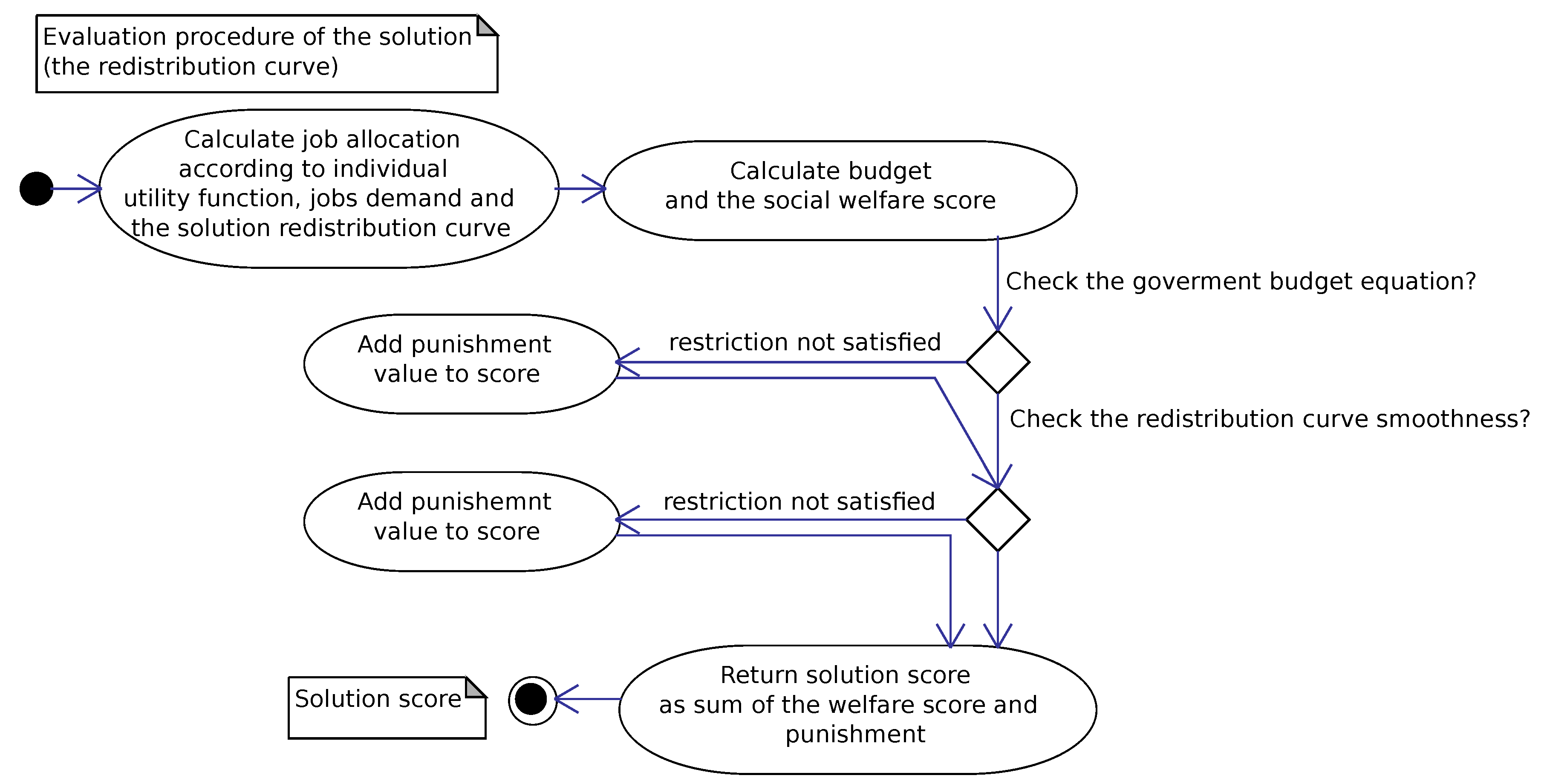
In addition to the list of operators used in optimization, there are also some constraints on each child solution. One constraint restricts the node values of the redistribution curve to ensure that they do not violate the boundary constraints of the problem definition. A different constraint is used to test the angle between all triples of adjacent nodes. If the angle is below the threshold value, the modification is applied. This constraint ensures that all children created have an acceptably regular redistribution curve with no values that radically differ from node to node. It is assumed that constraints do not force the equation of the budget balance because it balances itself during optimization (the redistribution is preferable to accumulating money in the budget).

Once a child solution has been produced, the labor allocation algorithm assigns the labor to population members. After it, the child is assessed and a social welfare score is calculated as shown in Figure 9. If the solutions do not violate the budget constraint, then the social welfare value is the result of the goal function. Otherwise, a high punishment value is added to the social welfare value. This penalty in practice eliminates such a child solution from the winning population, since even a low-quality solution with a balanced budget is considered preferable. However, in certain circumstances, such approach helps to pass genetic material from infeasible parents to feasible offspring. It can improve the generality of the search process. The evaluation score determines the target cascade sub-population where the child would be placed. A pattern of possible migration paths for offspring is illustrated in Figure 8.

At the beginning of the search, the population has to be filled with initial (possibly feasible) solutions. Such solutions can be retrieved e.g., by generation of a set of random feasible tax schedules similar to proportional one. The algorithm producing initial solution uses the following equation:

$$R_d\left(g\right)=z\left(g\right)·s+m\left(g\right),$$

(11)

where $z\left(g\right)$ is the node income before taxation (it is related to $R_b\left(g\right)$), s is the random scaling variable reflecting the tax rate, $m\left(g\right)=m(g-1)+m_c$—component introducing nonlinearity to the tax schedule, and $m_c$ is a randomly chosen constant.

A better performance of the initial solutions’ generator was achieved by operating it in two modes. These modes are switched repeatedly after few iterations. In the first mode, the generator takes the best solution from the population. It modifies it slightly in a random way and adds the offspring to the population. This measure gives a chance to obtain a similar or even better solution. Then, in the second mode, a whole randomly created curve is added to the population if it is feasible. Although this algorithm delivers only very rough approximation of the final solution, it ensures in fact a better start position for the optimization that follows.

The algorithm has been implemented in the Java programming language as an application. It uses input data containing information on income brackets and corresponding population densities. The current version supports only one type of taxpayer. However, it is possible to extend the algorithm to operate on various subgroups of taxpayers (e.g., in the case of families). We also made an initial implementation of the model of the influence of the labor market on VAT and tax collection costs.

5. Conclusions

The proposed model of optimal income taxation is a reformulation of the model proposed in Mirrlees (1971) prepared for stochastic optimization. Departure from purely algebraic methods for finding the optimal solution has allowed the consideration of more complex relationships and interactions in the simulated economy. Thus, it was possible to include in the model many dependencies and extensions that cannot be formulated using simple functions reflecting cost models or labor markets. Moreover, many possible extensions of the proposed real economy-inspired model can easily be accommodated due to the declarative nature of the stochastic model. They include indirect taxes (e.g., VAT, capital taxes), sub-populations with different utilities (e.g., families, complex compositions of allowances), and various costs related to the tax system. Considering these extensions may lead to the discovery of new nontrivial relationships in the tax system or help to confirm some existing and actually observed real-life properties.

Simulations performed in a more realistic context may enable the application of the theory of optimal income taxation. However, this would require a more elaborate model using accurate data describing the actual population, larger populations of representatives in the simulation, and settings that reduce the granularity (e.g., finer skills and labor scales). Nevertheless, we obtained experimental results that align to findings described in Sadka (1976) and Heathcote and Tsujiyama (2019). Thus, our model can reveal properties of the optimal tax problem like more traditional approaches.

Finally, to complete the picture, it is necessary to point out some disadvantages of the proposed approach. They arise from the fact that the proposed stochastic method does not guarantee success in finding the global optimum. It is even difficult to verify whether the obtained solution is actually the optimal globally. This problem becomes more important as the number of dimensions of the explored search space increases. Therefore, the criteria for acceptability of the solution must be determined on the basis of the social welfare score.

Our experimental results suggest the following tax policy guidelines:

• Decision makers should encourage people to work and invest in employees’ competences (in our model expressed as skills—the ability to earn money). Funding social incentives for workers instead of encouraging them to work could put the economy into a downward spiral. It also imposes a relatively higher tax burden on middle-class people, which in turn makes some services, such as healthcare and education, more expensive. Our model shows that a positive attitude to work directly reduces the rate of the income tax which has further positive impact on the consumption and the overall economy development.
• The government should optimize and limit unnecessary expenses. This is the second important point that was shown in our results. The government should pursue a consistent policy of cutting spending, as it affects the poor more than the rich. Otherwise, the threshold at which poorer people can be offered social grants is narrowing and overall tax rates are rising sharply, even for the poor.
• The third experiment shows that the richest taxpayer segment has relatively little impact on the social welfare outcome. We obtained many solutions with a similar welfare score and different tax rates at the high earning end. At the same time, tax rates for the middle and low-income part of the population remain relatively stable. The result suggests that social transfer takes place mainly between the middle class and poor people. On the other hand, the direct impact of the narrow, the richest class on average social welfare in the population is relatively small (even if their tax contribution is not low). It is worth noting that our model ignores what the richest class do with the excess money—for example, how their untaxed money is invested (including where it is spent), and what impact this could have on the economy and labor market structure. We believe that the empirical answer to this question is crucial when determining tax rates for the richest taxpayers.

In our opinion, implications of micro-simulation may not be always directly applicable to macroeconomic policy-making due to a gap in the complexity of both systems. They should be seen as a guide and not as a directly applicable solution, as there are many other factors influencing economic policy that are not covered by the simplified models. However, even in this case, the knowledge derived from their results can give decision makers valuable insight into the properties of the process.