1. Introduction
Recently, the market for cryptocurrencies has exhibited one of the most volatile periods in its history. While the total market capitalisation for cryptocurrencies reached a record high of over USD 800 billion in the last quarter of 2017, it was followed by a massive correction in the market leading to significantly reduced market capitalisation, which now stands at under USD 100 billion. This clearly suggests that the market has experienced a bull (cryptocurrency-price rising, precrisis) and bear (cryptocurrency-price falling, crisis) market throughout this period. Overspeculation, and interest from academics and those in the industry in this new financial technology are a few reasons behind this recent market phenomenon.
Over the past few years, the cryptocurrency literature has been rapidly expanding. The general literature on cryptocurrencies covers topics including (but not limited to) statistical analysis, modelling, and predicting the Bitcoin/USD exchange rate, measuring the volatility of the Bitcoin exchange rate against different financial assets and commodities, stylised facts of cryptocurrencies, and the market efficiency of cryptocurrencies.
Chu et al. (
2015) provided the first statistical and risk modelling analysis on Bitcoin returns. The generalized hyperbolic distribution provided the best fit;
Glaser et al. (
2014) investigated whether Bitcoin users see it as a currency or asset, and found that most uninformed users were not interested in Bitcoin as a transaction system but instead saw it as an alternative investment method.
Kristoufek (
2013) investigated the relationship between Bitcoin prices and search queries from Google and Wikipedia. They found that there was a significant positive correlation between prices and search queries, and that search queries had asymmetric effects on Bitcoin prices depending on whether prices were above or below the short-term trend. The significant volatility in Bitcoin prices and returns cannot simply be explained by economic or financial theory.
Sapuric and Kokkinaki (
2014) analysed the volatility of the exchange rate of Bitcoin during its early years and found that it was significantly greater than that of major exchange rates. However, when they accounted for transaction volume, volatility appeared to be more stable.
Baur et al. (
2018) analysed the statistical properties of Bitcoin and found that they were “uncorrelated with traditional asset classes such as stocks, bonds, and commodities, both in normal times and in periods of financial turmoil”. In addition, the authors found that Bitcoin is primarily used as an investment asset and not as a currency.
Briere et al. (
2015) investigated Bitcoin from an investment perspective and found that it had significantly high average return and volatility, and little correlation with traditional financial assets. Results showed that, by including Bitcoin in well-diversified portfolios, the risk-return trade-off could be significantly improved.
The efficient market hypothesis (EMH) is a core and fundamental concept used in finance that was introduced by
Malkiel and Fama (
1970) through modelling financial data. There are three main forms of efficiency, with the most common being the weak form. The weak form states that investors cannot use historical-price information to make future-price predictions. The importance of understanding market efficiency can be beneficial to investors, academics, and financial practitioners, as historical-price pattern information can assist in the greater understanding or discovery of arbitrage returns. On the other hand, liquidity is a concept of how easily capital and assets can be traded without causing a dramatic change in an asset’s price. In general, an illiquid asset would procure a higher bid ask spread and transaction cost, increasing the cost for speculators and investors to trade. Hence, if cryptocurrency markets are very illiquid, this results in market inefficiency, as the lack of market makers and traders causes a delay in market participants acting on new information.
Many attempts were made so far to study the market efficiency of various cryptocurrency markets, but the vast majority of the known work has been exclusively directed towards the Bitcoin market. For example,
Bariviera (
2017) studied the long-range memory of the Bitcoin market by analysing the Hurst exponent via the R/S and detrended-fluctuation-analysis (DFA) methods, and confirmed that daily volatility exhibits long-range memory;
Alvarez-Ramirez et al. (
2018) implemented the DFA method to estimate the long-range dependence of Bitcoin and found that the Bitcoin market exhibited periods of efficiency, alternating in different periods;
Tiwari et al. (
2018) reported that the Bitcoin market is informationally efficient, by using a battery of robust long-range dependence estimators;
Khuntia and Pattanayak (
2018) examined the efficiency of the Bitcoin market by using the Dominguez–Lobato consistent test and generalized spectral test, and concluded that dynamic efficiency in the Bitcoin market actually follows the proposition of adaptive market hypothesis (AMH);
Jiang et al. (
2018) employed the generalised Hurst exponent to investigate long-term memory in the Bitcoin market, and results suggested that the Bitcoin market was inefficient over the whole sample period;
Zhang et al. (
2018a) illustrated that the nine most popular cryptocurrency markets were inefficient by employing a battery of efficiency tests, and the MF-DFA and MF-DCCA approaches;
Zhang et al. (
2018b) analysed the stylised facts of cryptocurrencies in terms of long-range dependence by using the Hurst exponent with both the R/S and DFA methods for high-frequency-return data of the four most popular cryptocurrencies, while features of dependence between the different cryptocurrencies were also provided;
Chu et al. (
2019) analysed the efficiency of the high-frequency markets of the two largest cryptocurrencies, Bitcoin and Ethereum, versus the euro and US dollar, by investigating the existence of the AMH.
Our main motivation was to analyse and understand market-efficiency patterns and liquidity behaviour during a bull (precrisis) and bear (crisis) market for cryptocurrencies. These periods are very intriguing as they represent different market conditions. The main contributions of this paper are: (i) utilising algorithms for detecting turning points to identify bull and bear phases for the three largest cryptocurrencies of Bitcoin, Ethereum and Litecoin in high-frequency (hourly) markets; and (ii) analysing and understanding the characteristics of market efficiency and liquidity in high-frequency cryptocurrency returns during a bull or bear market. This is the first study of detecting bull and bear periods in high-frequency cryptocurrency markets, and analysing their market efficiency and liquidity during such periods.
For each cryptocurrency, we analysed data from 1 July 2017 to 19 September 2018. This time period was divided into two subperiods, corresponding to a bull market (precrisis period) from 1 July 2017 to 16 January 2018 (4789 observations), and a bear market (crisis period) from 17 January 2018 to 19 September 2018 (5888 observations).
Section 2 and
Section 3 provide a detailed justification of how the bull and bear markets were identified.
For each cryptocurrency, we performed analysis by using two different methods. The first was to apply the DFA method to compute the Hurst exponent over a rolling window during a bull and bear market to analyse the behaviour of the high-frequency (hourly) returns of Ethereum, Bitcoin and Litecoin. The DFA method is most commonly implemented by using a rolling-window approach for analysing the Hurst exponent in financial time series (see, for example,
Matos et al. 2008,
Grech and Mazur 2004, and
Carbone et al. 2004). The second was to use a series of tests, presented in
Section 2, which examined the efficient market hypothesis within fixed periods (bull and bear markets). A rolling-window approach splits a dataset into subsamples of a specific size rather than analysing the whole data sample in one process. The initial subsample is analysed before the next most recent data are added to the subsample, and the earliest data in the subsample are removed. This process is then repeated until the subsample reaches the most recent data in the whole sample. A conventional fixed-period method analyses the whole data sample in one go.
The contents of the paper are organised as follows. The algorithms used in detecting bull and bear markets in cryptocurrencies and the methods used to measure the long-range memory, liquidity, and market efficiency of cryptocurrencies in a bull and bear market are discussed in
Section 2. The three cryptocurrency datasets and their summary statistics are described in
Section 3. Data analysis using a range of different methods, including analysis of the Hurst exponent, is presented in
Section 4. Finally, conclusions are drawn in
Section 5.
3. Data
In this paper, the datasets that we used consisted of historical high-frequency (hourly) prices of cryptocurrencies versus the US Dollar (USD) from 11:00 on 11 July 2017 to 00:00 on 19 September 2018 inclusive. The data were obtained from
CryptoCompare (
2018), and our analysis was limited to data that were available for download at the time. We chose cryptocurrencies for our analysis on the basis of the most popular cryptocurrencies traded on the GDAX exchange during that time, namely, Bitcoin, Ethereum, and Litecoin. These three cryptocurrencies accounted for around 80% of total market capitalisation for cryptocurrencies during that period, and we could therefore assume that the used datasets provide an adequate representation of the market.
Chan et al. (
2017) provides more details on the individual cryptocurrencies.
Before analysis, our preliminary approach in determining the bull and bear run period was to first identify the highest point (peak) in the dataset, which occurred on 16 January 2018. We then classified all data points prior to the peak (from 1 July 2017 to 16 January 2018) as being part of a general bull run in the market, and all points after the peak (17 January 2018 to 19 September 2018) as part of a general bear market run. However, to theoretically justify our selected periods, we implemented the
Bry and Boschan (
1971) and
Lunde and Timmermann (
2004) algorithms using the parameter values mentioned in
Section 2 for detecting bull and bear periods.
There are numerous software packages that could be implemented to detect bull and bear markets in financial data, and in this analysis we use the R statistical software package (2019). To implement the ‘dating’ and ‘filtering’ algorithm methods introduced by
Bry and Boschan (
1971), and
Lunde and Timmermann (
2004), respectively, in R, we used R package
bbdetection. The parameter values for the two methods were set using the two commands
setpar_dating_alg and
setpar_filtering_alg, respectively. For the dating algorithm, we selected parameter values of
For the filtering algorithm, we selected parameters of
Our reasoning for the values of , , and was to have a consistent threshold relating to price changes in both methods to detect peaks and troughs to determine the start and end of bull- and bear-market states. In the dating algorithm, was selected so that, at each time point, only turning points in the one week before and after were considered. The remainder of the parameter values were chosen to remove bull- and bear-market states that were only short-lived and insignificant.
Figure 1 plots the results of these algorithms in detecting bull and bear periods in cryptocurrency data. The shaded-white (grey) areas identify periods of a bull (bear) market run in the cryptocurrency data. The top-left (-right) diagram in
Figure 1 shows the result through implementing the dating (filtering) algorithm, respectively, for Ethereum. The majority of the area before the peak for both approaches has a greater proportion of shaded-white areas than grey, which indicates that, in general, the market was a bull market. In contrast, the period after the peak sees a greater proportion of shaded-grey areas, which suggests that the market was more of a bear market in that period. Similar results were also seen for Bitcoin and Litecoin using the dating and filtering algorithms. Hence, the results used in this analysis support our preliminary results. This provides us with a reasonable case for selecting our chosen time periods for the bull and bear periods in our main analysis.
Table 1 and
Table 2 provide summary statistics of log returns of high-frequency (hourly) market prices during a bull and bear market. In
Table 1, the summary statistics of the log returns of the market-price index for Ethereum, Bitcoin, and Litecoin versus USD in a bull market are given. The BTC/USD index had the highest minimum, first quartile, median, and mean, while it had the lowest third quartile, maximum, and range. In contrast, the LTC/USD index had the lowest minimum, first quartile, and median, while it had the highest mean, third quartile, maximum, and range. Bitcoin was the only negatively skewed cryptocurrency. All cryptocurrencies showed significantly greater peakedness than normal distribution, and the LTC/USD index gave the highest kurtosis value. In terms of index spread, the values of standard deviation and variance for all cryptocurrencies were fairly similar (almost 0).
Table 2 presents summary statistics of log returns of market price index for Ethereum, Bitcoin, and Litecoin versus USD during a bear market. Similar to
Table 1, the BTC/USD index had the highest minimum, first quartile, median, and mean, while it had the lowest third quartile, maximum, and range. Litecoin had the lowest minimum, first quartile, and median, and the highest maximum and range. Once again, all cryptocurrencies showed significantly greater peakedness than normal distribution, and the LTC/USD index gave the highest kurtosis value. Compared with bull-market summary statistics, all cryptocurrencies were positively skewed, and Litecoin had the largest skewness value. With regard to variation, ETH/USD gave the greatest standard deviation and variance. Standard deviation and variance values of log returns for all cryptocurrencies were very small and close to 0.
By comparing
Table 1 and
Table 2, there was significant difference in some statistical properties between bull and bear markets. Compared with the bull market, the values of the minimum, skewness, and kurtosis for all cryptocurrencies increased during the bear market. However, the coefficient of variation for all cryptocurrencies significantly decreased, changing from positive to negative values. The interquartile range (IQR) for all cryptocurrencies also decreased in the bear market, implying that the middle
of data during the bear market were less spread out.
4. Results and Discussion
Table 3,
Table 4 and
Table 5 show the results of the various test for the efficient market hypothesis on Ethereum, Bitcoin, and Litecoin, respectively. These tests were conducted over two fixed subperiods, during the bull market and during the bear market. In each case, corresponding
p-values are shown. For the bull-market period, the majority of the
p-values (with the exception of the Runs test for Ethereum and the AVR test for Litecoin) for all cryptocurrencies rejected the null hypotheses of no autocorrelation, independence, and random walk. Similarly, during the bear-market period, the majority of the
p-values (with the exception of the Ljung–Box test and AVR test for Ethereum) for all cryptocurrencies rejected the null hypotheses of no autocorrelation, independence, and random walk. Overall, these tests indicated that high-frequency (hourly) cryptocurrency returns exhibited behaviour consistent with an inefficient market during both a bull and bear market. When compared to other financial markets, similar results can be seen, for example,
Gil-Alana et al. (
2018) noted that the Baltic stock market rejected the theory of market efficiency during the bull and bear markets;
Jiang and Li (
2019) investigated market efficiency for the Chinese, Japanese, and U.S. stock markets, and found market inefficiency in both the bull- and bear-market states, which could be explained by behavioural finance theory.
The results of Amihud’s illiquidity ratio are shown in
Table 6. Results were multiplied by
for a simpler comparison, and this did not lead to loss of information. When comparing the three cryptocurrencies on the basis of the Amihud ratio, Bitcoin had the smallest value, followed by Ethereum and Litecoin. This illustrates that Bitcoin is the most liquid cryptocurrency. This result is consistent with our expectations, as Bitcoin holds the largest share of the cryptocurrency-market capitalisation, making it the most actively traded cryptocurrency. Other factors that led to Bitcoin being the most actively traded cryptocurrency include numerous trading platforms requiring users to hold Bitcoin before being able to trade other cryptocurrencies; the launch of Bitcoin futures, which allowed speculators to long and short Bitcoin and increased Bitcoin volatility; and the majority of exchanges providing other products, such as the trading of cryptocurrency pairs (e.g., BTC/ETH, BTC/LTC, BTC/XRP), with the majority of pairs involving Bitcoin.
When comparing bull- and bear-market liquidity and volatility, there was a strong relationship between liquidity and volatility for Ethereum and Litecoin. For Ethereum and Litecoin, market volatility decreases during a bear market, and the market becomes less liquid. However, results were different for Bitcoin, as market volatility decreases during a bear market, and Bitcoin becomes more liquid than in the bull market. This phenomenon could be explained by investors becoming irrational and worrying about the whole cryptocurrency market collapsing, leading to a majority of investors cashing out their cryptocurrency holdings. Most trading exchanges only allow cashing out cryptocurrencies through Bitcoin; therefore, this also causes Bitcoin to be traded by more active traders, which makes the market more liquid.
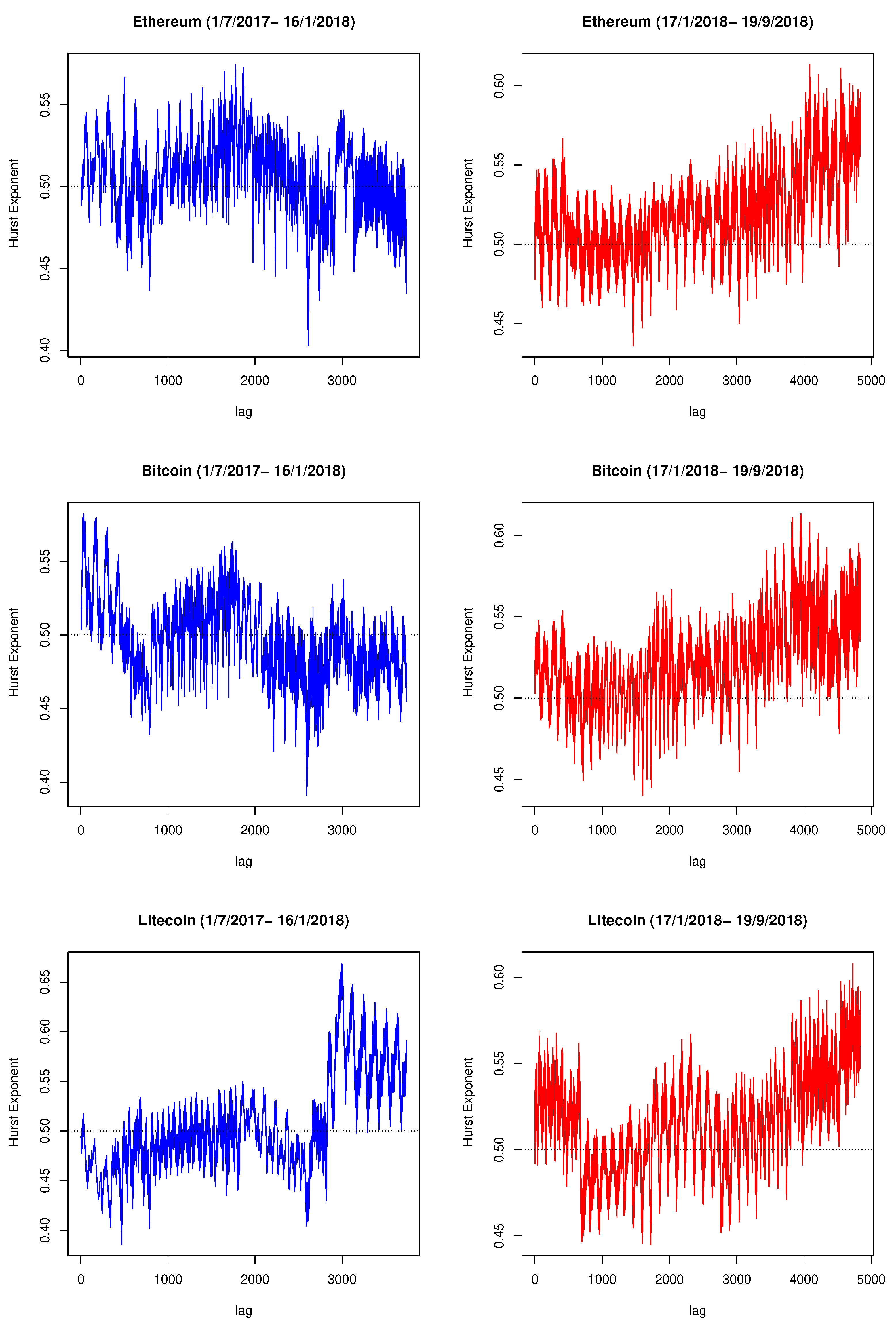
The long-range memory for all three cryptocurrencies during a bull and bear market was computed using the DFA method. The difference between this and previous methods is that this technique uses a rolling-window approach, as discussed in
Section 2. A dotted black line in each plot was included to enable easier comparison between plots.
Figure 2, illustrates the fluctuating behaviour of the Hurst exponent for the hourly returns of Ethereum, Bitcoin, and Litecoin during the different market periods. Ethereum and Bitcoin Hurst exponent values follow a similar pattern during the bull and bear market. In contrast, Litecoin results look slightly different. Throughout the bull period, Ethereum and Bitcoin generated a Hurst exponent of around 0.5, with Ethereum being slightly higher than Bitcoin. However, at around 2700 lags (bull period), the value significantly drops to below 0.4 before correcting and fluctuating back to around 0.5. In general, a Hurst exponent close to 0.5 indicates that the series is more random and resembles a random walk. This suggests that hourly Ethereum and Bitcoin returns are relatively efficient during a bull market. During the bear market, Ethereum and Bitcoin exhibit an increasing trend in the Hurst exponent as lag times increase. This indicates that the returns of both cryptocurrencies experience long-term positive autocorrelation. For Litecoin, the pattern of the Hurst exponent during a bull market is very close to 0.5 for the first 3000 lags, which illustrates that returns follow a random walk. However, after 3000 lags, the Hurst exponent suddenly increases to a value over 0.6, suggesting persistent behaviour. During a bear market, Litecoin exhibits a similar pattern to Bitcoin and Ethereum, suggesting that the market experiences long-term positive autocorrelation. Overall, we can conclude that, during a bull market, cryptocurrencies exhibit random-walk behaviour. However, when a bear market occurs, returns start to show persistent positive autocorrelation behaviour (market inefficiency). These results are also in line with those of
Wang and Yang (
2010), who identified intraday market inefficiency in heating-oil and natural-gas energy future markets during bull-market states, but not during bear markets.
A contrast in results from both methods during the bull-market phase could be interpreted in the following way. Analysis involving the Hurst exponent utilises a rolling-window approach; during these individual rolling windows (subsamples of a specific size) within the bull market, the cryptocurrency market had actually steadily grown with investors gradually entering the market, thus leading to an efficient-market phenomenon. However, if we look at the overall picture of the bull-market phase, we see the market significantly rises; when considering the method that uses a fixed sample period, this appears to create an inefficient market. On the contrary, during the bear-market phase, the price consistently decreased throughout the whole period, which may have caused panic and irrational trading by investors, leading to a downward spiral in market prices, resulting in market inefficiency.
The actual methods and tests used here could also lead to result divergence due to the difference in tested samples in each case. For example, methods such as the Ljung–Box, Runs, and Bartels tests analyse all bull-/bear-market phase data as one, as opposed to the DFA method that analyses dynamic rolling data windows from the bull-/bear-market periods. In other words, the size of the samples analysed by the DFA method is smaller, but data points vary, while samples used in general tests are larger and data are fixed. Therefore, it is possible that the DFA method picks up variations within particular subsamples of return data (thus affecting results relating to market efficiency), which may be masked when considering bull-/bear-market samples as a whole. Furthermore, our results illustrate that, in a bear market, hourly Bitcoin returns become more liquid during this period of market inefficiency. In contrast, hourly Ethereum and Litecoin returns exhibit less liquidity in this period.
Here, we only tested the hypothesis of market efficiency through a range of different tests (including classical tests and the DFA method). We cannot claim that the DFA is better or more trustworthy, but results of DFA analysis suggest that the level of market efficiency is different in bull and bear markets. Although the Hurst exponent (as a proxy for market efficiency) shows general trends in bull and bear markets, there are shorter-term changes that are also captured, likely due to the rolling-window approach. One could run the classical tests over different sample periods, but a problem that remains is that classical tests only generate a p-value. This p-value only gives us an indication of whether we can reject or fail to reject the null hypothesis of tests for properties such as independence, autocorrelation, and random walk. This is in contrast to DFA analysis, which not only gives us a numerical value indicating deviations from market inefficiency, but could provide further information, such as trend-reinforcing or antipersistence behaviour.
5. Conclusions
We provided the first analysis for detecting bull and bear markets for the three largest cryptocurrencies of Bitcoin, Ethereum, and Litecoin in high-frequency (hourly) markets using algorithms on the basis of
Lunde and Timmermann (
2004) and
Bry and Boschan (
1971). Results from
Section 4 showed that hourly returns of Ethereum, Bitcoin, and Litecoin during a bull market exhibited a random walk (market efficiency) when using a rolling DFA Hurst exponent test. However, when conditions changed and the market entered a bear-market period, we saw signs that the market started to show persistence positive autocorrelation behaviour (market inefficiency).
In addition, we utilised six different tests to investigate market efficiency using a nonrolling fixed period. During the bull- and bear-market periods, the hourly returns of the three cryptocurrencies exhibited market inefficiency.
Similar results could be seen for other financial markets, for example,
Gil-Alana et al. (
2018) noted that the Baltic stock market rejected the theory of market efficiency during bull- and bear-market states;
Jiang and Li (
2019) investigated market efficiency for the Chinese, Japanese, and U.S. stock markets, and found market inefficiency in bull- and bear-market states. Furthermore, the Amihud illiquidity ratio illustrated that, in a bear market, hourly Bitcoin returns become more liquid. In contrast, hourly Ethereum and Litecoin returns exhibit less liquidity in this period compared to during a bull-market period.
In addition, we saw that volatility of hourly returns of all three cryptocurrencies decreased during a bear market. There is much scope for future work, and possible extensions could include: (i) focusing not only on hourly, but also higher-frequency data (minutes) due to movement towards higher-frequency cryptocurrency trading; (ii) further investigations into how these results for bull and bear markets could be used for arbitrage or trading strategies, for example, if there is inefficiency in the market during particular periods, if we could use market properties to monitor and predict when it would be the best time to buy or sell; (iii) investigate how to define bull and bear periods in a high-frequency market. Theoretically, there are many short bull- and bear-market periods within our two subsamples, so this may be more useful if we are considering trading at a higher-frequency level.
References


