Bootstrapping the Early Exercise Boundary in the Least-Squares Monte Carlo Method

Abstract

This paper proposes an innovative algorithm that significantly improves on the approximation of the optimal early exercise boundary obtained with simulation based methods for American option pricing. The method works by exploiting and leveraging the information in multiple cross-sectional regressions to the fullest by averaging the individually obtained estimates at each early exercise step, starting from just before maturity, in the backwards induction algorithm. With this method, less errors are accumulated, and as a result of this, the price estimate is essentially unbiased even for long maturity options. Numerical results demonstrate the improvements from our method and show that these are robust to the choice of simulation setup, the characteristics of the option, and the dimensionality of the problem. Finally, because our method naturally disassociates the estimation of the optimal early exercise boundary from the pricing of the option, significant efficiency gains can be obtained by using less simulated paths and repetitions to estimate the optimal early exercise boundary than with the regular method.

1. Introduction

Simulation and regression based methods are by now standard methods used for American option pricing. Simulation methods are flexible, work in multiple dimensions, can be used with even the most complicated models and payoff functions, and are straightforward to use. Essentially, if you can simulate it (the underlying dynamics), you can price it (the derivatives contract).1 Moreover, under standard assumptions, the estimates have nice properties since averages over independent samples converge to expected values. Almost all the simulation methods that have been proposed for American option pricing share the feature that in one way or another, they involve estimating or approximating the early exercise boundary or, more generally, estimating or approximating the conditional expectations that are used to decide whether or not to exercise at each step.2 In the Least-Squares Monte Carlo (LSM) method of Longstaff and Schwartz (2001), for example, the conditional expectations are approximated with polynomials, and based on these approximations, it is then decided at each early exercise point and along each simulated path whether the option should be exercised or not; implicitly determining the early exercise region.

While the asymptotic properties of the LSM method are well established (see for example (Stentoft 2004b)), the quality of the price estimate obtained with this method depends on the order of the polynomial, M, used in the cross-sectional regression and the number of paths, N, used in the simulation (see, e.g., Moreno and Navas 2003; Stentoft 2004a). With a finite choice of polynomial terms, M, and simulated paths, N, the early exercise boundary is estimated with some error. Because of this, sub-optimal decisions are made, and everything else equal, low biased price estimates are obtained. Moreover, because sub-optimal decisions are made early on, errors are propagated backwards through the algorithm. This paper presents an innovative bias reduction technique directly applicable to the LSM method, as well as to many other similar methods. The method successfully delivers at each early exercise step, starting from just before maturity, a “better” estimated early exercise boundary. Because of this, less errors are accumulated, and by recursively correcting the estimated optimal early exercise boundary, we end up with essentially unbiased price estimates even for long maturity options.

To motivate our methodology, we first demonstrate that significantly less biased estimates can be obtained if the precision of the early exercise boundary is improved upon by simply averaging it over several independently repeated simulations. Next, we show that by averaging at each step, and therefore obtaining a less noisy estimate of the early exercise strategy, less errors are propagated backwards through the algorithm. Our method is based on the simple observation that if one uses the average of the approximated early exercise strategies instead of, say, the $I=100$ individually determined strategies, the estimated prices are much closer to the benchmark prices. Our proposed method exploits and leverages this observation to the fullest by averaging at each step in the backwards induction algorithm instead of only after having gone through all the steps of the backward induction algorithm. We refer to our method as a bootstrapping approach because of the similarities it has with how the term structure of interest rates is bootstrapped and the way bootstrapping is used for inference in regression models. As a result of the bootstrapping approach, the final bias of the estimated price is almost completely eliminated.

We compare the results from our bootstrapping approach to the regular method of Longstaff and Schwartz (2001) and show that our proposed method works extremely well across various levels of moneyness, maturity, and volatility. Moreover, compared to the regular LSM method, the bootstrapping method is much less sensitive to the choice of polynomial order used in the cross-sectional regressions and to the number of paths used in the Monte Carlo simulation. When a reasonable order, say $M=9$, is used in the regressions and when a standard number of paths, say $N=$ 100,000, is used in the simulation, our proposed method essentially provides unbiased price estimates. We also demonstrate that the technique generalizes straightforwardly to multi-asset options with various payoffs. To illustrate this, we price arithmetic and geometric average options and options on the maximum and minimum of three assets. For all four payoff functions, the results hold, and the bootstrapped method always performs the best and delivers price estimates with negligible or very small bias for reasonable choices of the number of regressors and paths used in the Monte Carlo simulation.

Our method successfully corrects the bias even in very small samples and allows for using, e.g., $N=$ 10,000 paths or less to determine the early exercise boundary. Our detailed results also show that one does not need hundreds of repeated simulations to obtain a good estimate of the early exercise boundary, but a much lower number, e.g., $I=10$ suffices. Determining the early exercise boundary is the most computationally complex part of the algorithm since this involves performing several cross-sectional regressions, and our method therefore offers significant computational speedups. For example, one can run $I=10$ initial simulations with $N=$ 10,000 paths to estimate the optimal early exercise boundary. One can then use $N=$ 1,000,000 paths for pricing, whereby an estimate with very low bias and low variance is obtained. Note that in this setup, obtaining the initial estimate of the optimal early exercise boundary takes no more time than running the standard LSM method once, and since it is straightforward to parallelize our method, it could run in a fraction of this time on multicore processors or modern computer clusters.

It should be noted that several papers have proposed alternative refinements to this type of simulation method. In particular, it has been suggested to use well known variance reduction techniques like antithetic simulation, control variates, importance sampling, as well as initial dispersion together with the LSM method (see, among others: (Juneja and Kalra 2009; Lemieux and La 2005; Rasmussen 2005)). However, there are very few alternative suggestions for how to reduce the bias of the simulated estimates of American option prices in general and of the LSM method in particular. One potentially interesting method, which could be combined with our method, is that of Kan et al. (2009), although their application was to the value function iteration method of, e.g., Carriere (1996) and Tsitsiklis and Van Roy (2001). Our proposed method could also be used together with the inequality constrained least-squares method suggested in Létourneau and Stentoft (2014) or the method that corrects for heteroskedasticity in the cross-sectional regression proposed by Fabozzi et al. (2017).

Finally, our current applications are to standard financial options, but our results have important implications for other applications of simulation based pricing as well. One particularly important and challenging area in which the LSM method has been used is the field of real option valuation. For example, the work in Gamba and Fusari (2009) proposed a general valuation approach for capital budgeting decision involving modularization, and the work in Kang and Létourneau (2016) studied the investment decision and choice between coal and natural gas power plants under political risk with options to turn production on or off, while the work in Power et al. (2015) studied the valuation and timing of complex infrastructure projects. In all these cases, the regular LSM method was used to approximate complex decision problems in settings with multiple risk factors with complicated dynamics and for problems where the payoff function is non-standard and “exotic”. We conjecture that our proposed bootstrapping method will allow more efficient determination of the optimal controls and more precise valuation of these assets.

The remainder of the paper is structured as follows: Section 2 describes the discrete time framework used for valuation, introduces the least-squares Monte Carlo method of Longstaff and Schwartz (2001), and demonstrates how our proposed bootstrapping method can be implemented and improves estimation of the early exercise boundary. Section 3 presents an extensive numerical analysis of the performance of our proposed method demonstrating its robustness to changes in the simulation setup, to different option characteristics, and its applicability to higher dimensional problems. Section 4 provides a discussion of the potential benefits of separating the estimation of the early exercise boundary from the pricing and demonstrates that our method can be implemented in a very efficient way that works well in empirically relevant settings. Section 5 concludes.

2. Framework

The first step in implementing a numerical algorithm to price early exercise options is to assume that time can be discretized. We specify J exercise points as $t_0=0<t_1\le t_2\le \dots \le t_J=T$, with $t_0$ and T denoting the current time and maturity of the option, respectively. Thus, we are essentially approximating the American option by the so-called Bermudan option. The American option price is obtained in the limit by increasing the number of exercise points, J; see also Bouchard and Warin (2012) for a formal justification of this approach.3 We assume a complete probability space $\left(\mathsf{\Omega },\mathcal{F},\mathbb{Q}\right)$ equipped with a discrete filtration ${\left(\mathcal{F}\left(t_j\right)\right)}_{j=0}^J$ and a unique pricing measure corresponding to the probability measure $\mathbb{Q}$. The derivative’s value depends on one or more underlying assets modeled using a Markovian process, with state variables ${\left(X\left(t_j\right)\right)}_{j=0}^J$ adapted to the filtration. We denote by ${\left(Z\left(t_j\right)\right)}_{j=0}^J$ an adapted discounted payoff process for the derivative satisfying $Z\left(t_j\right)=\pi \left(X\left(t_j\right),t_j\right)$ for a suitable function $\pi \left(·,·\right)$ assumed to be square integrable. This notation is sufficiently general to allow for non-constant interest rates through the appropriate definition of the state variables X and the payoff function $\pi$ (see, e.g., Glasserman 2004). Following, e.g., Karatzas (1988) and Duffie (1996), in the absence of arbitrage, we can specify the American option price as:

$$P\left(X\left(0\right)=x\right)=\underset{\tau \left(t_1\right)\in \mathcal{T}\left(t_1\right)}{max}\mathrm{E}\left[Z\left(\tau \right)|X\left(0\right)=x\right],$$

(1)

where $\mathcal{T}\left(t_j\right)$ denotes the set of all stopping times with values in $\{t_j,\dots ,t_J\}$. Thus, we explicitly assume that the option cannot be exercised at time $t=0$.

The problem of calculating the option price in (1) with $J>1$ is referred to as a discrete time optimal stopping time problem and typically solved using the dynamic programming principle. Intuitively this procedure can be motivated by considering the choice faced by the option holder at time $t_j$. The optimal choice will be to exercise immediately if the value of this is positive and larger than the expected payoff from holding the option until the next period and behaving optimally onwards. Let $V\left(X\left(t_j\right)\right)$ denote the value of the option for state variables X at a time $t_j$ prior to expiration and define $F\left(X\left(t_j\right)\right)\equiv \mathrm{E}\left[Z\left(\tau \left(t_{j+1}\right)\right)\right|X\left(t_j\right)]$ as the expected conditional payoff, where $\tau \left(t_{j+1}\right)$ is the optimal stopping time. It then follows that:

$$V\left(X\left(t_j\right)\right)=max\left(Z\left(t_j\right),F\left(X\left(t_j\right)\right)\right),$$

(2)

and the optimal stopping time can be derived iteratively as:

$$\begin{array}{c}\left\{\begin{array}{c}\tau \left(t_J\right)=T\hfill \\ \tau \left(t_j\right)=t_j{\mathbf{1}}_{\{Z\left(t_j\right)\ge F\left(X\left(t_j\right)\right)\}}+\tau \left(t_{j+1}\right){\mathbf{1}}_{\{Z\left(t_j\right)<F\left(X\left(t_j\right)\right)\}},\hfill & 1<j\le J-1.\hfill \end{array}\right.\end{array}$$

(3)

Based on this stopping time, the value of the option in (1) can be calculated as:

$$P\left(X\left(0\right)=x\right)=\mathrm{E}\left[Z\left(\tau \left(t_1\right)\right)|X\left(0\right)=x\right].$$

(4)

The backward induction theorem of Chow et al. (1971) (Theorem 3.2) provides the theoretical foundation for the algorithm in (3) and establishes the optimality of the derived stopping time and the resulting price estimate in (4).

2.1. Simulation and Regression Methods

The idea behind using simulation for option pricing is quite simple and involves estimating expected values and, therefore, option prices by an average of a number of random draws. However, when the option is American, one needs to determine simultaneously the optimal early exercise strategy, and this complicates matters. In particular, it is generally not possible to implement the exact algorithm in (3) because the conditional expectations are unknown, and therefore, the price estimate in (4) is infeasible. Instead, an approximate algorithm is needed. Because conditional expectations can be represented as a countable linear combination of basis functions, we may write $F\left(X\left(t_j\right)\right)={\sum }_{m=0}^{\infty }{\varphi }_m\left(X\left(t_j\right)\right)c_m\left(t_j\right)$, where ${\left\{{\varphi }_m\left(·\right)\right\}}_{m=0}^{\infty }$ form a basis.4 To make this operational we further assume that the conditional expectation function can be well approximated with the first $M+1$ terms such that $F\left(X\left(t_j\right)\right)\approx F_M\left(X\left(t_j\right)\right)={\sum }_{m=0}^M{\varphi }_m\left(X\left(t_j\right)\right)c_m\left(t_j\right)$ and that we can obtain an estimate of this function by:

$${\widehat{F}}_M^N\left(X\left(t_j\right)\right)=\sum _{m=0}^M{\varphi }_m\left(X\left(t_j\right)\right){\widehat{c}}_m^N\left(t_j\right),$$

(5)

where the coefficients ${\widehat{c}}_m^N\left(t_j\right)$ are approximated or estimated using $N\ge M$ simulated paths. For example, in the Least-Squares Monte Carlo (LSM) method of Longstaff and Schwartz (2001), these are determined from a cross-sectional regression of the discounted future path-wise payoff on transformations of the state variables.

Based on the estimate in (5), we can derive an estimate of the optimal stopping time as:

$$\begin{array}{c}\left\{\begin{array}{c}{\widehat{\tau }}_M^N\left(t_J\right)=T\hfill \\ {\widehat{\tau }}_M^N\left(t_j\right)=t_j{\mathbf{1}}_{\{Z\left(t_j\right)\ge {\widehat{F}}_M^N\left(X\left(t_j\right)\right)\}}+{\widehat{\tau }}_M^N{\mathbf{1}}_{\{Z\left(t_j\right)<{\widehat{F}}_M^N\left(X\left(t_j\right)\right)\}},\hfill & 1<j\le J-1.\hfill \end{array}\right.\end{array}$$

(6)

From the algorithm in (6), a natural estimate of the option value in (4) is given by:

$${\widehat{P}}_M^N\left(X\left(0\right)=x\right)=\mathrm{E}\left[Z\left({\widehat{\tau }}_M^N\left(1\right)\right)\right|X\left(0\right)=x].$$

(7)

In the special case when all the paths are started at the current values of the state variables, i.e., $X\left(0\right)=x$, the conditional expectation in (7) can be estimated by the sample average given by:

$${\widehat{P}}_M^N\left(X\left(0\right)=x\right)=\frac{1}{N}\sum _{n=1}^{N}Z\left(n,{\widehat{\tau }}_M^N\left(1,n\right)\right),$$

(8)

where $Z\left(n,{\widehat{\tau }}_M^N\left(1,n\right)\right)$ is the payoff from exercising the option at the estimated optimal stopping time ${\widehat{\tau }}_M^N\left(1,n\right)$ determined for path n according to (6). Convergence of this type of estimate has been analyzed in detail in the existing literature. The first step in doing so is to establish the convergence of the estimated approximate conditional expectation function, which is done in, e.g., the following lemma.

Lemma 1

(Adapted from Theorem 2 of Stentoft 2004b). Under some regularity and integrability assumptions on the conditional expectation function, F (see Stentoft (2004b) for details), if $M=M\left(N\right)$ is increasing in N such that $M\to \infty$ and $M^3/N\to 0$, then ${\widehat{F}}_M^N\left(X\left(t_j\right)\right)$ converges to $F\left(X\left(t_j\right)\right)$ in probability for $j=1,\dots ,J$.

Proof. 

See Stentoft (2004b). □

The result in Lemma 1 can now be combined with Proposition 1 of Stentoft (2004b) to demonstrate that when all the simulated paths are started at the current values of the state variable, i.e., $X\left(0\right)=x$, then the estimate in (8) converges to the true price, which establishes the convergence of the LSM method in a general multi-period setting.5 Moreover, this type of algorithm has nice properties, and the work in Stentoft (2014) documented that it is the most efficient method when compared to, e.g., the value function iteration method of Carriere (1996) or Tsitsiklis and Van Roy (2001). When paths are started at initially dispersed values, the LSM method still allows one to estimate the optimal early exercise boundary, and Lemma 1 continues to hold. However, when it comes to pricing the option with initially dispersed paths, this is more complicated, and an initial regression is needed at time $t=0$; see, e.g., Létourneau and Stentoft (2019) for a proof that this method converges.

2.2. Regression and Optimal Early Exercise

It is explicit in Equation (3) that the optimal early exercise region is determined by the comparison of $Z\left(t_j\right)$ and $F\left(X\left(t_j\right)\right)$ or in the case when the conditional expectations are approximated by the comparison of $Z\left(t_j\right)$ and ${\widehat{F}}_M^N\left(X\left(t_j\right)\right)$. In particular, we can define the true early exercise region implicitly as the value $B\left(t_j\right)$ that solves:

$$Z\left(t_j\right)>F\left(B\left(t_j\right)\right).$$

(9)

Similarly the estimated early exercise region is defined as the value ${\widehat{B}}_M^N\left(t_j\right)$ that solves:

$$Z\left(t_j\right)>{\widehat{F}}_M^N\left({\widehat{B}}_M^N\left(t_j\right)\right).$$

(10)

In the case where there is only one state variable, the exercise region at an exercise date is determined by a single point of intersection between the payoff function and conditional expectation. The work in Rasmussen 2005 proposed a Newton–Raphson procedure to find the exercise boundary. In our application, we find this exercise boundary by subtracting the exercise value from the approximated conditional expectation and determining the roots of the resulting polynomial. Note that with an approximated conditional approximation, multiple roots may exist. If this happens, the largest root below the strike is kept as the exercise boundary.

While it is simple to find and represent the optimal early exercise boundary in the plain vanilla single option case, for more complex options, this might not be the case. For example, when there are two state variables, the conditional expectations and payoff functions are planes in a three-dimensional space. Hence, the intersection is a curve in a three-dimensional space, and it becomes much more difficult to represent the intersection.6 Moreover, while finding polynomial roots is easy in one dimension, this approach does not generalize easily to more complex situations. On the other hand, comparing the payoff function to the approximated conditional expectation is straightforward in multiple dimensions. Since the conditional expectations are completely described by the estimated coefficients ${\widehat{c}}_m^N\left(t_j\right)$ from the cross-sectional regression, in practical implementations, it is therefore much easier to store these than it is to attempt to characterize and store a representation of the exercise region.

It follows from Lemma 1 above that as M and N tend to infinity, the estimated early exercise boundary will converge to the true early exercise boundary. For finite choices, however, ${\widehat{B}}_M^N\left(t_j\right)$ is only an estimate of the true early exercise boundary, and the “quality” of this estimate will depend on the choice of M and N in a particular application. The fact that the early exercise boundary is estimated leads to two types of biases. First, when using a given estimated frontier, the option may be exercised at times when it should not have been or not exercised at times when it should have been. In both cases, this suboptimal early exercise will result in a low biased price estimate.7 Second, when using the same set of simulated paths to the approximation of the exercise boundary and to price the option, what we call in-sample pricing, the method suffers from a high bias from over-fitting the continuation value to the current sample of simulated paths. As explained first by Broadie and Glasserman (1997), the practice of using the same paths for the exercise decision and the payoff calculation introduces a positive correlation between the exercise decision and the future payoffs, essentially resulting in a foresight bias. The standard LSM estimator has both the low and the high bias, and therefore, the overall bias is difficult to sign.

2.3. Bootstrapping the Early Exercise Boundary

Although simulation and regression methods like the LSM method outlined above determine sequentially a number of conditional expectations as can be seen from Equation (6), these are used only to determine if the option at a given time should be exercised along a given path. As such, the conditional expectations are used as a convenient way to summarize, by subtracting the exercise value, the early exercise region and hence the path-wise optimal stopping time, which uniquely determines the option value. In Figure 1a, we plot in light gray $I=100$ such estimated early exercise boundaries for a put option. As the figure shows, these are close to the true optimal early exercise boundary with the dotted black line although quite noisy, and this particularly so at the first steps in the simulation. Figure 1a however also shows that taking averages of the $I=100$ conditional expectation approximations at any time and using that to back out the optimal early exercise boundary leads to a much smoother frontier shown with the dotted blue line and, supposedly, a better behaved estimated price.

Our proposed bootstrapping technique averages at each step in the backwards induction algorithm instead of only after having gone through all the steps in the backward induction algorithm. For example, at time $t=T-1$, we estimate $I=100$ independent conditional expectation approximations, i.e., polynomials of order $M=9$ and a constant term in the cross-sectional regressions. Before proceeding backwards, we take the average of these approximations and use this same average across the $I=100$ independent simulations to determine if the option along a given path in a given simulation at time $t=T-1$ should be exercised or not. We then simply proceed, in a similar manner, backwards in time, always averaging at each early exercise point to time $t=0$. In Figure 1a, we show in red the early exercise boundary backed out from these average conditional expectations at each early exercise time. This estimated optimal early exercise boundary is for the most part extremely close to the true optimal early exercise boundary, and estimated option prices obtained with this estimate are therefore expected to be very close to the true option price.

In

Table 1. Option prices using In-Sample (IS) and Out-of-Sample (OS) methods. LSM, Least-Squares Monte Carlo.

	Using IS Method		Using OS Method		Difference
Benchmark Boundary	2.3150	(0.0084)	2.3137	(0.0080)	0.0013
Individual LSM	2.3170	(0.0087)	2.3119	(0.0079)	0.0051
Regular Average	2.3148	(0.0085)	2.3136	(0.0079)	0.0013
Recursive Average	2.3150	(0.0084)	2.3138	(0.0080)	0.0012

This table shows the estimated prices and standard deviations using $I=100$ individually estimated early exercise boundaries using $N=$ 100,000 paths of simulated data with $M=9$ regressors and a constant term in the cross-sectional regressions. The option has a strike price of $K=40$, a maturity of $T=1$ year, and $J=50$ early exercise points per year. The initial stock price is fixed at $S\left(0\right)=40$; the volatility is $\sigma =20\%$; and the interest rate is $r=6\%$. The binomial model estimate obtained with 50,000 steps is $2.3141$. The benchmark boundary denotes the results from a method in which the true early exercise boundary estimated from the binomial model is used in the Monte Carlo simulation. Individual LSM denotes the regular method where the average of the $I=100$ individual simulations are used. Regular average denotes the method where the average of the individually estimated optimal early exercise strategy is used, and recursive average denotes the method where the bootstrapped estimated optimal early exercise strategy is used. By comparing these results to the values from the benchmark boundary, the error coming from the Monte Carlo simulation is eliminated.

, we report the corresponding price estimates using both In-Sample (IS) pricing, i.e., when the same paths are used to determine the optimal early exercise boundary and for pricing, and Out-of-Sample (OS) pricing, where new simulated stock prices are used for pricing. A benefit of using OS pricing in the LSM method is that the price estimate is guaranteed to have a low expected bias because of the sub-optimality of the estimated optimal early exercise boundary. The first line in the table reports the relevant benchmark values for both the IS and OS method generated by applying the true early exercise boundary estimated from the binomial model with 50,000 steps to the relevant simulated paths. In this case, the IS and OS simply represent two different sets of paths. The table shows that as expected, the regular LSM method provides a high biased estimate when using IS and a low biased estimate when using OS, and these differences are in fact significant at standard levels.8 The difference between the two estimates is about half a cent, though slightly less when factoring in the Monte Carlo error as evidenced by the difference of $0.0013$ between the benchmark price using the IS and OS sample. For the methods based on averages, the table shows that the estimated prices, both IS and OS, are much closer to the benchmark values and insignificantly different. This is particularly so for the recursive averages based on our bootstrapping method, which are spot on for the IS method and off by only a hundredth of a cent for the OS method. This indicates that for this setup, we have essentially obtained the true optimal early exercise strategy with our proposed bootstrapping method.

The very jagged paths early on in the simulations in Figure 1a are due in part to there being very few paths that are deep in the money, which makes it difficult to estimate the value for which exercise is optimal. This can be corrected or improved upon by using Initial State Dispersion (ISD) as suggested by, e.g., Rasmussen (2005). The resulting estimated early exercise boundaries are shown in Figure 1b. Compared to Figure 1a, we see that using an ISD helps quite a bit for the individual early exercise boundaries, which are quite a bit less volatile up to the 25th early exercise points. However, while using an ISD may help when estimating the individual optimal early exercise boundaries, comparing the two figures clearly shows that bootstrapping helps much more.

The method we propose is simple to implement and yields very good results with finite choices of the number of regressors used in the simulation, the number of simulated paths, and the number of repeated independent simulations. A natural next step is to ask about the asymptotic properties of this algorithm. It is straightforward to show that our method provides asymptotically unbiased price estimates, which we state in the following corollary.

Corollary 1.

The bootstrapping method provides an asymptotically unbiased estimate of the option price for any choice of I, i.e., the number of repeated independent simulations used, under the assumptions outlined in Lemma 1.

Proof. 

This follows by applying Lemma 1 to each of the independent simulations and noting that since the individual ${\widehat{F}}_M^N\left(X\left(t_j\right)\right)$ converge to $F\left(X\left(t_j\right)\right)$ in probability for $j=1,\dots ,J$ so does the average of I such simulations. □

3. Results

The previous section demonstrated how our bootstrapping method can be implemented and shows that it leads to much more precise estimates of the optimal early exercise boundary and results in estimated prices that are essentially unbiased for a benchmark option. In this section, we test the robustness of these findings along several dimensions. First, we show that our results are robust across choices in the simulation setup for the number of regressors and the number of paths used and across option characteristics like the moneyness and maturity of the option and the volatility of the underlying asset. To illustrate this, we consider first options on a single stock in a simple model with Black–Scholes–Merton dynamics because this allows us to characterize the true optimal early exercise boundary, which can be used to obtain Monte Carlo benchmark values. Finally, we show that our results generalize to the case with multiple underlying assets. We consider four different payoffs, and though the pricing performance varies across payoffs and depends on the order of the polynomial approximation, our bootstrapped method performs the best across different approximations.9

3.1. Robustness to the Simulation Setup

In Section 2.3, we demonstrated how to implement the bootstrapping method for a given number of regressors, $M=9$, and number of simulated paths, $N=$ 100,000. However, both M and N are choice parameters in the simulation setup that need to be picked when implementing the method. Thus, the first thing we analyze is the robustness of our proposed method to the choice of the number of simulated paths, N, used for determining the estimated optimal early exercise boundary and subsequently for pricing in case the OS method is used. The option we consider here has a strike price of $K=40$, a maturity of $T=1$ year, and $J=50$ early exercise points per year. The initial stock price is fixed at $S\left(0\right)=40$; the volatility is $\sigma =20\%$; and the interest rate is $r=6\%$. For now, we continue to use a polynomial of order $M=9$ in the cross-sectional regressions.

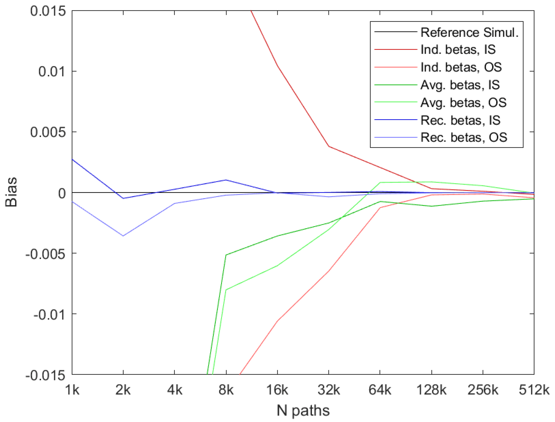
Figure 2 compares the results from using the three different methods to determine the estimated optimal early exercise boundary: the regular LSM method, the regular average of the individual LSM boundaries, and the recursively bootstrapped boundaries, as a function of the number of simulated paths, N. The red lines represent the average price over $I=100$ independent repetitions of the LSM method, each of which uses N paths. The line above the benchmark reference uses the IS method, whereas the line below uses the OS method. To eliminate the sampling bias from using a finite number of paths in the Monte Carlo simulation, we compare the price estimates to what would be obtained using the true early exercise boundary backed out from a binomial model with 50,000 steps on the two sets of simulated paths. The green lines use the regular average over the $I=100$ individual LSM repetitions using N paths, and the blue lines use the recursive average over $I=100$ individual LSM repetitions using N paths.

First, the figure clearly shows that the regular IS LSM price can be strongly biased if the number of paths is too low. This is due to using the same paths to determine the individual optimal early exercise boundary and for calculating payoffs, which as we discussed earlier, leads to a high bias in the estimated option price. The OS prices, i.e., from the method that uses a new set of paths for pricing, are guaranteed to be low biased as shown in the figure. As the number of paths used in the individual simulation increases, the IS and OS results converge to a value that is (slightly) lower than the benchmark value, but corresponds to the true approximate value obtained when the approximation $F_M\left(X\left(t_j\right)\right)$ based on a polynomial of order $M=9$ of the true conditional expectation $F\left(X\left(t_j\right)\right)$ is used.

Next, the figure shows that using the regular average method over the $I=100$ repetitions improves on the results when a low number of paths is used. This is the situation where the early exercise boundary is estimated with the most noise, and averaging helps counter that somewhat. Note that the IS prices for this method are also low biased because of the averaging. As expected, both price estimates converge to the true approximated price as the number of paths used increases and in the limit, which in our setting corresponds to using $N=$ 512,000 paths; averaging has very little effect on the estimated prices.

The final and most interesting thing the figure shows is that using the recursive average dramatically improves on the results across all values of N. In fact, Figure 2 essentially shows that the recursive method is virtually unbiased, even when using as little as $N=1000$ paths to approximate the conditional expectations. Using only $N=1000$ paths for OS pricing with the estimated early exercise boundary also leads to unbiased estimates, although both of these estimates will naturally have quite large variances.

In addition to N being a choice parameter for the LSM method, so is M. In Figure 3, we plot equivalent results to those in Figure 2, but using $M=5$ and $M=15$, respectively. The first thing to notice is that the two plots in Figure 3 show a pattern that is very similar to that obtained when using $M=9$ in Figure 2. For example, the LSM method is high biased when using IS pricing and low biased when using OS pricing with $M=5$, as well as with $M=15$. Figure 3, however, does indicate that these biases are larger for a given value of N when $M=15$ than when $M=5$. This is expected since the degree of overfitting increases with M. This also affects the method that averages the optimal early exercise boundaries somewhat, although our bootstrapping method is much less effected. In particular, our proposed method works very well for both $M=5$ and $M=15$, even when a low number of simulated paths, N, is used in the simulation.

3.2. Robustness across Option Characteristics

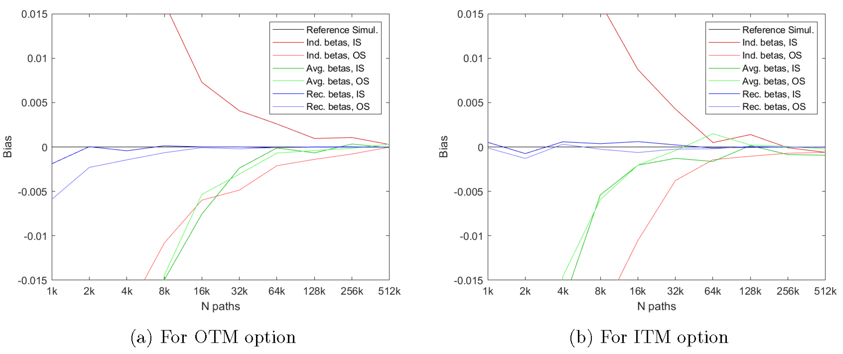
We now demonstrate that our previous findings are robust to considering options with different moneyness, maturity, and volatility of the underlying asset. To examine this, we consider additional options with strike prices of $K=36$ and $K=44$, maturities of $T=0.5$ and $T=2$ years, and volatilities of the underlying of $\sigma =10\%$ and $\sigma =40\%$. Again, we assume that the options have $J=50$ early exercise points per year, such that the option with $T=0.5$ years maturity has 25 early exercise points and the option with $T=2$ years maturity has 100 early exercise points, respectively. We keep the number of regressors fixed at $M=9$, but plot the resulting price estimates as a function of the number of simulated paths, N.

Figure 4 shows the performance of the three methods for an Out of The Money (OTM) option with $K=36$ in the left hand plot and for an In The Money (ITM) option with $K=44$ in the right hand plot. The first thing to notice is that the two plots in Figure 4 show a pattern that is very similar to that obtained for the At The Money (ATM) option with $K=40$ in Figure 2. Figure 4 does indicate, though, that the biases in the LSM method are larger for a given value of N when pricing an OTM option than when pricing an ITM option. This is expected since the degree of overfitting increases as we go out of the money where less paths are used in the cross-sectional regressions. However, our proposed method continues to work very well, and much better than the regular LSM method, for both OTM and ITM options even when a low number of simulated paths, N, is used in the simulation.

Figure 5 shows the performance of the three methods for a Short Maturity (ST) option with $T=0.5$ years to maturity and 25 early exercise points in the left hand plot and for a Long Maturity (LT) option with $T=2$ years to maturity and 100 early exercise points in the right hand plot. The first thing to notice is again that the two plots in Figure 5 show a pattern that is very similar to that obtained for the option with a maturity of $T=1$ year in Figure 2. Figure 5 does indicate, though, that the biases in the LSM method are larger for a given value of N when the maturity of the option increases. This is to be expected since errors in the approximation of the conditional expectations accumulate in the backward algorithm, and we thus expect larger accumulated errors for longer maturities. However, our proposed method continues to work very well, and much better than the regular LSM method, for both ST and LT options even when a low number of simulated paths, N, is used in the simulation.

Figure 6 shows the performance of the three methods for an option on an asset with a low volatility of $\sigma =10\%$ in the left hand plot and for an option on an asset with a high volatility of $\sigma =40\%$ in the right hand plot. Again, the first thing to notice is that the two plots in Figure 6 show a pattern that is very similar to that obtained for the option on an underlying asset with a volatility of $\sigma =20\%$ in Figure 2. Figure 6 does indicate, though, that the biases in the LSM method are larger for a given value of N when the volatility of the underlying asset increases. However, our proposed method continues to work very well, and much better than the regular LSM method, for both options on low and high volatility assets even when a low number of simulated paths, N, is used in the simulation.

3.3. Robustness to the Dimensionality of the Problem

We now demonstrate that our previous findings for options on a single asset are robust when increasing the number of underlying assets. To examine this, we consider options on three underlying assets with payoffs on the arithmetic average, the geometric average, the maximum, and the minimum of the underlying assets. We consider options that are at the money with $K=40$ and a maturity of $T=0.5$ years, and have $J=25$ early exercises in total. The underlying asset prices are $S_i\left(0\right)=40$; the volatilities are ${\sigma }_i=40\%$, for $i=1,2,3$; the correlation between all assets is $\rho =0.5$; and the interest rate is $r=6\%$. Benchmark prices are obtained with a binomial model with 2000 steps a year. Since it is difficult to characterize explicitly the optimal early exercise boundary for these options, we compare to the true price, and we therefore cannot take the Monte Carlo error into consideration.

Figure 7 shows the price estimates for options with the four different payoff across the number of paths used in the simulation, N. In all cases, the complete set of polynomials of order $M=9$ and a constant term are used as regressors in the cross-sectional regressions. The first thing to note is that in all cases the algorithms converge, though for options on the maximum and minimum, this is to a somewhat low biased estimate. This makes sense since the conditional expectations are more difficult to approximate for these options; see also Stentoft (2004a). More importantly, though, for all the payoffs, our proposed bootstrapping method delivers the least biased price estimates. Thus, the results clearly show that our proposed method is robust to increases in the dimension of the pricing problem.

To demonstrate further our method’s robustness, Figure 8 shows the corresponding price estimates when the maximum order of the complete polynomial is $M=15$, in which case a total of 816 regressors are used in the cross-sectional regressions. It is possible that by using other regressors, e.g., functions of the maximum asset value, than the complete set of polynomials, better results could be obtained with less regressors; however, for consistency and simplicity, we chose to stay with monomials as the basis. The figure shows that when M is increased, the asymptotic bias, apparent when using a very large number of simulated paths N, decreases, and this is particularly so for the maximum and minimum options. Note though that for all payoffs, our proposed bootstrapping method again continues to perform the best and deliver price estimates with the lowest bias of all the methods reported.

4. Discussion

The results in Section 3 were obtained by averaging over $I=100$ repeated samples with the same number of simulated paths, N, for both IS and OS pricing. In this section, we first demonstrate that it is in fact not necessary to average over such a large number of repeated samples when bootstrapping the optimal early exercise boundary. We also show that it is in fact not necessary to average over independently repeated simulations with a large number of simulated paths in the bootstrapping method either.10 Finally, since the number of repeats, $I_{IS}$, and the number of simulated paths, $N_{IS}$, used for IS pricing can be disassociated from the number of repeats, $I_{OS}$, and number of simulated paths, $N_{OS}$, used for OS pricing, we propose to price options using our proposed bootstrapping method with reasonably low values for $I_{IS}$ and $N_{IS}$, since this is enough to obtain unbiased results, and large values of, in particular, $N_{OS}$, since this will deliver price estimates with a low variance.11

Figure 9 shows that the quality of the approximation of the estimated early exercise boundary very quickly improves, reflected in decreasing absolute bias of the estimated price, as $I_{IS}$ and $N_{IS}$ increase. In fact, if as little as $I_{IS}=10$ repeats and $N_{IS}=$ 10,000 simulated paths are used, the OS bias is very small, and when $I_{IS}=10$ repeats and $N_{IS}=$ 50,000 simulated paths are used, it is essentially eliminated. Note that estimating the optimal early exercise boundary with $I_{IS}=10$ repeats and $N_{IS}=$ 10,000 simulated paths can be done in roughly the same time as running the regular LSM method once with $N=$ 100,000, a number typically used.12

To illustrate the efficiency of our method, we now report for all combinations of moneyness, maturity, and volatility, a total of 27 options, the estimated prices from implementing our bootstrapping method with $I_{IS}\ll I_{OS}$ and $N_{IS}<N_{OS}$. Specifically, we set $I_{IS}=10$ and $N_{IS}=$ 50,000 and price the options out of sample with $I_{OS}=100$ and $N_{OS}=$ 100,000, the standard choice in the literature. Compared to the regular LSM method, the IS results can be calculated in a fraction of the time (5% roughly) with our bootstrapping method. The results are reported in

Table 2. Option prices using bootstrapping.

			Benchmark Boundary		Recursive Average
$\mathbf{K}$	$\mathbf{T}$	$\mathbf{\sigma }$	Price	St. Dev.	Price	St. Dev	Difference
36	0.5	10%	0.0304	(0.0006)	0.0303	(0.0006)	−0.0000
36	1	10%	0.0896	(0.0012)	0.0894	(0.0012)	−0.0001
36	2	10%	0.1715	(0.0018)	0.1714	(0.0018)	−0.0001
36	0.5	20%	0.4974	(0.0035)	0.4971	(0.0035)	−0.0003
36	1	20%	0.9169	(0.0052)	0.9166	(0.0052)	−0.0003
36	2	20%	1.4317	(0.0069)	1.4311	(0.0071)	−0.0006
36	0.5	40%	2.1978	(0.0104)	2.1972	(0.0102)	−0.0006
36	1	40%	3.4360	(0.0135)	3.4355	(0.0134)	−0.0006
36	2	40%	4.9619	(0.0168)	4.9606	(0.0169)	−0.0013
40	0.5	10%	0.7344	(0.0029)	0.7343	(0.0029)	−0.0000
40	1	10%	0.8892	(0.0031)	0.8891	(0.0032)	−0.0001
40	2	10%	1.0235	(0.0038)	1.0234	(0.0038)	−0.0001
40	0.5	20%	1.7907	(0.0072)	1.7907	(0.0071)	−0.0001
40	1	20%	2.3137	(0.0080)	2.3133	(0.0079)	−0.0005
40	2	20%	2.8833	(0.0099)	2.8824	(0.0099)	−0.0009
40	0.5	40%	3.9708	(0.0144)	3.9697	(0.0144)	−0.0010
40	1	40%	5.3115	(0.0170)	5.3103	(0.0168)	−0.0011
40	2	40%	6.9149	(0.0210)	6.9131	(0.0210)	−0.0017
44	0.5	10%	3.9474	(0.0019)	3.9474	(0.0019)	−0.0000
44	1	10%	3.9473	(0.0018)	3.9472	(0.0018)	−0.0001
44	2	10%	3.9480	(0.0020)	3.9480	(0.0019)	−0.0000
44	0.5	20%	4.3079	(0.0094)	4.3078	(0.0093)	−0.0001
44	1	20%	4.6528	(0.0098)	4.6523	(0.0098)	−0.0005
44	2	20%	5.0804	(0.0112)	5.0796	(0.0116)	−0.0008
44	0.5	40%	6.3232	(0.0176)	6.3228	(0.0176)	−0.0005
44	1	40%	7.6107	(0.0200)	7.6095	(0.0197)	−0.0011
44	2	40%	9.1784	(0.0232)	9.1764	(0.0233)	−0.0020

This table shows estimated prices and standard deviations using our proposed bootstrapping method. The OS method is used with $I_{OS}=100$ and $N_{OS}=$ 100,000 with IS recursive averages calculated with $I_{IS}=10$ and $N_{IS}=$ 50,000 with $M=9$ regressors, and a constant term in the cross-sectional regressions. The option characteristics are given in the first 3 columns. In all cases, the initial stock price is fixed at $S\left(0\right)=40$; the options have $J=50$ early exercise points per year; and the interest rate is $r=6\%$. The benchmark boundary denotes the results from a method in which the true early exercise boundary estimated from the binomial model with 50,000 steps is used in the Monte Carlo simulation. By comparing the results to the values from the benchmark boundary, the error coming from the Monte Carlo simulation is eliminated. The differences are shown in the last column.

, which compares the bootstrapped results to the results that would be obtained had the true optimal early exercise boundaries been used.

Table 2 shows that all the estimated prices are low biased, which is expected since we are using OS pricing. However, the absolute size of the bias is indeed very small, and in all cases, the bias is statistically insignificant. Across the 27 options, the largest bias in absolute value is $-0.0020$, well below a cent, and the average bias across the sample of options is $-0.0005$. Moreover, the table shows that the standard deviations of our estimated prices are similar to what is obtained when applying the benchmark frontier. Thus, when pricing this sample of diverse and empirically relevant options, our bootstrapping method essentially yields unbiased price estimates that are as precise as if the true optimal early exercise boundary had been used. If the regular LSM method had been used instead, the corresponding biases, both the largest ones and the average across options, would have been much larger and more volatile.13 Note that the option for which the bias is the largest is the long term in the money option on a high volatility underlying asset. The results in Section 3 demonstrate that this is the most challenging option to price with the regular LSM method, and in light of this, our bootstrapping method performs remarkably well.

The constant volatility Gaussian models considered above may not be adequate for empirical option pricing. Thus, to check the robustness of our results to more realistic alternatives, we now consider models with time varying volatility of the GARCH type. The work in Duan (1995) was among the first to show how to price options in a (Gaussian) GARCH model, and this framework has since been widely used empirically. See Christoffersen et al. (2013) for a detailed survey of the use of GARCH option pricing models. In the GARCH option pricing model, returns under the pricing measure $\mathbb{Q}$ are given by:

$$R_t=r-\frac{1}{2}{h}_t+{\epsilon }_t,$$

(11)

where ${\epsilon }_t\mid {\mathcal{F}}_{t-1}\sim N\left(0,h_t\right)$, with ${\mathcal{F}}_t$ denoting the information set at time t and where the conditional variance, $h_t$, follows a NGARCH process given by:

$$h_{t+1}=\omega +\beta h_t+\alpha \left({\epsilon }_t-\left(\lambda +\gamma \right)\sqrt{h_t}\right),$$

(12)

where $\omega$, $\beta$, $\alpha$, and $\gamma$ are parameters governing the dynamics under the physical measure $\mathbb{P}$ and $\lambda$ is the constant unit risk premium. The GARCH model is obtained when $\gamma =0$, and the constant volatility model amounts to setting all parameters except $\omega$ equal to zero.

Table 3. Option prices with time varying volatility.

Panel A: Constant Volatility Model
	Individual LSM					Recursive Average
K	Price	St. Dev.	Bias	T-stat		Price	St. Dev.	Bias	T-stat
36	0.4983	(0.0036)	−0.0011	−2.8281		0.4990	(0.0036)	−0.0004	−1.0196
40	1.7936	(0.0068)	−0.0021	−2.9162		1.7945	(0.0066)	−0.0012	−1.6947
44	4.3158	(0.0075)	−0.0018	−2.2127		4.3171	(0.0073)	−0.0005	−0.6237
Panel B: GARCH Model
	Individual LSM					Recursive Average
K	Price	St. Dev.	Bias	T-stat		Price	St. Dev.	Bias	T-stat
36	0.5060	(0.0037)	−0.0021	−5.4783		0.5076	(0.0037)	−0.0005	−1.3202
40	1.7725	(0.0068)	−0.0031	−4.3681		1.7747	(0.0069)	−0.0009	−1.2259
44	4.2844	(0.0074)	−0.0030	−3.7376		4.2873	(0.0074)	−0.0001	−0.1330
Panel C: NGARCH model
	Individual LSM					Recursive Average
K	Price	St. Dev.	Bias	T-stat		Price	St. Dev.	Bias	T-stat
36	0.5822	(0.0045)	−0.0026	−5.4823		0.5842	(0.0044)	−0.0005	−1.1326
40	1.7431	(0.0072)	−0.0035	−4.6303		1.7454	(0.0071)	−0.0012	−1.5857
44	4.1799	(0.0072)	−0.0036	−4.7237		4.1826	(0.0072)	−0.0010	−1.2543

This table shows estimated prices and standard deviations using the individual LSM method and our proposed bootstrapping method for models with time varying volatility of the GARCH type. The OS method is used with $I_{OS}=100$ and $N_{OS}=$ 100,000 with the complete set of polynomials of order $M_S=5$ and $M_V=3$ in the stock price and the volatility, respectively, in the cross-sectional regressions. The individual LSM uses the same numbers in the IS method, whereas the recursive averages are obtained with $I_{IS}=10$ and $N_{IS}=50,000$. The option strike prices are given in the first column, and all options have a maturity of $T=0.5$ year and $J=252$ early exercise points per year. The initial stock price is fixed at $S\left(0\right)=40$; the volatility is $\sigma =20\%$; and the interest rate is $r=6\%$. The following parameters were used: $\beta =0.92$, $\alpha =0.05$, $\gamma =0.5$, and $\lambda =0.1$, and to ensure a risk neutral unconditional annual volatility of $20\%$, we set $\omega =\left(1-\beta -\alpha \left(1+{\left(\lambda +\gamma \right)}^2\right)\right)*0.20/\sqrt{252}$. Benchmark prices are calculated using $N=$ 1,000,000 paths and the complete set of polynomials of order $M_S=9$ and $M_V=5$ in the stock price and the volatility, respectively, in the cross-sectional regressions.

shows the results for three different volatility specifications and thus examines the robustness of our results to using more general stochastic processes. The first thing to notice from the table is that our proposed bootstrapping method generates price estimates with insignificant biases irrespective of the dynamic model used. Thus, the table demonstrates that the excellent performance of our proposed method does not depend on the complexity of the dynamics. Using the ordinary LSM method, however, leads to significantly biased price estimates, and this is particularly so when the conditional volatility follows the more complicated NGARCH process. Our proposed method, on the other hand, continues to deliver statistically insignificant price estimates when more complicated and empirically relevant dynamics are used, and the estimates are much less biased than with the ordinary LSM method.

5. Conclusions

This paper proposed an innovative algorithm that significantly improves on the approximation of the optimal early exercise boundary obtained with simulation based methods for American option pricing like, e.g., the Least-Squares Monte Carlo (LSM) method of Longstaff and Schwartz (2001). The method successfully exploited and leveraged the information in multiple cross-sectional regressions to the fullest by averaging the individually obtained estimates at each early exercise step, starting from just before maturity, in the backwards induction algorithm. We referred to our method as a bootstrapping approach because of the similarities it had with how the term structure of interest rates was bootstrapped and the way bootstrapping was used for inference in regression models. With the bootstrapping approach, less errors were accumulated in the backward induction algorithm, and as a result of this, the price estimate was essentially unbiased even for long maturity options.

We compared the results from our bootstrapping approach to the regular LSM method, and the numerical results demonstrated large and significant improvements from our method. These findings were robust to the choice of simulation setup, the characteristics of the option, and the dimensionality of the problem. Finally, because our method naturally disassociated the estimation of the optimal early exercise boundary from the pricing of the option, significant efficiency gains could be obtained by using less simulated paths and repetitions to estimate the optimal early exercise boundary than with the regular method. To illustrate this, we priced a diverse sample of options with different moneyness, maturity, and levels of volatility of the underlying asset. The results showed that when pricing this sample of empirically relevant options, our bootstrapping method essentially yielded unbiased price estimates that were as precise as if the true optimal early exercise boundary had been used.

Our bootstrapping method should have wide applications empirically. First, the majority of the options traded are in fact American style, and the recent global financial crisis clearly demonstrated that considering more risk factors is essential to model the complex behavior of financial markets properly. Our proposed method can be used with such advanced models and will allow more efficient pricing than what is currently possible. Second, our results have important implications for other simulation based applications. One particularly important and challenging area in which the LSM method has been used is the field of real option valuation. In particular, the dynamics of the underlying assets for this type of options are often very complicated, and simulation is the only viable method. We conjecture that our proposed bootstrapping method will allow more efficient determination of the optimal controls and more precise valuation of these assets, benefiting the economy at large.

Besides the empirical applications outlined above, there are other important lines for future research. First, we are currently working on establishing the finite sample properties of our proposed bootstrapping method to demonstrate theoretically its usefulness and to assess if there are any limitations to the applicability of the methodology. Second, simulation based methods have recently been used to obtain estimates of option risk sensitivities or hedge ratios, the Greeks, for American options. We conjecture that our bootstrapping method would allow such quantities to be estimated with much more precision as well and are currently working on establishing this empirically. Finally, our general idea could be applied to other methods that use simulation and regression techniques for pricing early exercise style option like, e.g., the value function iteration method of Carriere (1996) and Tsitsiklis and Van Roy (2001), and to other dynamic programming methods used to solve optimal control type problems.