Robust Bayesian Inference in Stochastic Frontier Models

Abstract

We use the concept of coarsened posteriors to provide robust Bayesian inference via coarsening in order to robustify posteriors arising from stochastic frontier models. These posteriors arise from tempered versions of the likelihood when at most a pre-specified amount of data is used, and are robust to changes in the model. Specifically, we examine robustness to changes in the distribution of the composed error in the stochastic frontier model (SFM). Moreover, coarsening is a form of regularization, reduces overfitting and makes inferences less sensitive to model choice. The new techniques are illustrated using artificial data as well as in a substantive application to large U.S. banks.

1. Introduction

The stochastic frontier model (SFM) is a standard tool in the estimation of efficiency from observed data. Robustness of SFM has not been examined thoroughly in the literature although many alternative distributional assumptions have been proposed for the error components of the model.1 Bayesian analysis of SFM is widely used due to the convenience allowed by Markov Chain Monte Carlo in dealing with latent inefficiencies that are present in the model, particularly under alternative distributional assumptions. Feng et al. (2019) proposed a semiparametric model for stochastic frontier models, specifically, the one-sided error term is approximated by a log-transformed Rosenblatt-Parzen kernel density estimator. In a Monte Carlo study, they found that that the kernel-based semiparametric model performs better than the commonly-used exponential stochastic frontier model. Their study also indicates that the kernel model shows similar performance to a non-parametric model.

Our motivation in this paper is to take into account the previous literature with an eye towards making the posterior (and, therefore, statistical inferences) more robust to misspecification. For example, standard inference in stochastic frontier models does not take into account not only outliers but, perhaps more importantly, deviations of the assumed distributions of two-sided and one-sided error terms from their actual counterparts. To the extent that the actual distributions are unknown (see, for example, Feng et al. 2019 for details) misspecification is quite likely so, in practice, statistical inferences are likely to be misleading.

A robust posterior, in the general case, has been proposed by Miller and Dunson (2019). Specifically, rather than conditioning on the observed data assumed to be generated by the model, we condition on the event that the model generates data that are distributionally close to the observed data. This technique allows examining robustness to changes in the distribution of the composed error in SFM. Additionally, coarsening is a form of regularization, reduces overfitting and makes inferences less sensitive to model choice. When we are interested in the estimation of efficiency, returns to scale, productivity growth, etc., this is clearly a desirable goal.

2. Model

Suppose we have observed data $x\in \mathcal{X}\subseteq {ℝ}^n$ and the “ideal” data is $X^{*}$-ideal in the sense that it is a random sample from the true data generating process (DGP). We focus on the case of i.i.d data whose distribution has density $p(x_i|\theta )$, where $\theta \in \mathsf{\Theta }\subseteq {ℝ}^M$ is a parameter and $\mathsf{\Theta }$ is the parameter space. The usual posterior $p(\theta |x)$ may not be robust if there are outliers and/or we are not certain that the density $p(x_i|\theta )$ is the true one.

A robust posterior is defined by Miller and Dunson (2019) in the i.i.d case as follows: $p(\theta |d\left({\widehat{P}}_{X^{*}},{\widehat{P}}_x\right)<r)$, where ${\widehat{P}}_x=n^{-1}{{\displaystyle \sum }}_{i=1}^n{\delta }_{x_i}$ is the empirical distribution of $x$ and similarly for ${\widehat{P}}_{X^{*}}$, for some discrepancy measure $D\left(\cdot ,\cdot \right)$ and a given $r>0$. Therefore, we condition on the event that the empirical distribution of actual data is close to the empirical distribution of data generated by the model, using a certain discrepancy function between probability measures.

If $P_o$ and $P_{\theta }$ for $\theta \in \mathsf{\Theta }$ have densities $p_o$ and $p_{\theta }$, respectively, the Kullback–Leibler divergence is defined as:

$$D\left(P_{\theta },P_o\right)={{\displaystyle \int }}_{\mathsf{\Theta }}{p}_o\left(\chi \right)\log \frac{p_o\left(\chi \right)}{p_{\theta }\left(\chi \right)}\lambda \left(d\chi \right),$$

(1)

where $\lambda$ is the Lebesgue measure. Miller and Dunson (2019) have derived the following approximation to the posterior under the assumption that $r$ has an exponential distribution with parameter $\alpha$:

$$p(\theta |d\left({\widehat{P}}_X,{\widehat{P}}_x\right)<r)\propto p\left(\theta \right){\displaystyle \prod }_{i=1}^{n}p{(x_i|\theta )}^{\zeta }\equiv p_{\zeta }(\theta |x),$$

(2)

where $\zeta =\frac{\alpha }{\alpha +n}$ and $p\left(\theta \right)$ is the prior. The approximation is accurate when $n\gg \alpha$ or $\alpha \gg n$. The main objective of such “coarsened” posteriors is robustness to small changes in the shape of the distribution of the data, i.e., the data generating process. The approximation avoids altogether computation of $D\left({\widehat{P}}_X,{\widehat{P}}_x\right)$ or the term ${{\displaystyle \int }}_{\mathsf{\Theta }}{p}_o\log p_o$ which is independent of $\theta$. The interpretation of the coarsened posterior is that it adjusts the sample size from $n$ to $n\zeta$, so effectively we have a smaller sample size.

In this paper we consider the production SFM2:

$$y_i={x^{\prime }}_i\beta +v_i-u_i,i=1,\dots ,n,$$

(3)

where $x_i\in {ℝ}^k$ is a vector of regressors, and $v_i\sim iid\mathcal{N}\left(0,{\sigma }_v^2\right),u_i\sim iid{\mathcal{N}}_{+}\left(0,{\sigma }_u^2\right),i=1,\dots ,n$, $\left(v_i,u_i\right)\perp x_i,i=1,\dots ,n$. Let ${\sigma }^2={\sigma }_v^2+{\sigma }_u^2$ and $\lambda =\frac{{\sigma }_u}{{\sigma }_v}$ and define the parameter vector $\theta ={[{\beta }^{\prime },{\sigma }_v,{\sigma }_u]}^{\prime }$. The augmented posterior is:

$$p(y_i,u_i|x_i,\theta )\propto {\sigma }_v^{-1}{\sigma }_u^{-1}\exp \left\{-\frac{1}{2{\sigma }_v^2}{\left(y_i+u_i-{x^{\prime }}_i\beta \right)}^2-\frac{1}{2{\sigma }_u^2}{u}_i^2\right\},i=1,\dots ,n.$$

(4)

The marginal density of $y_i$ is $p(y_i|x_i,\theta )={{\displaystyle \int }}_0^{\infty }p(y_i,u_i|x_i,\theta )d{u}_i$ and is available in closed form:

$$p(y_i|x_i,\theta )\propto {\sigma }^{-1}\exp \left\{-\frac{{(y_i-{x^{\prime }}_i\beta )}^2}{2{\sigma }^2}\right\}\mathsf{\Phi }\left(-\frac{\lambda }{\sigma }\left(y_i-{x^{\prime }}_i\beta \right)\right),i=1,\dots ,n,$$

(5)

where $\mathsf{\Phi }(\cdot )$ is the standard normal distribution function; see Kumbhakar and Lovell (2000, p. 78).

Suppose we have a prior $p\left(\theta \right)$ and $y=\left[y_i;i=1,\dots ,n\right]$, $X=\left[x_i;i=1,\dots ,n\right]$ denote the data. A coarsened posterior that uses at most $\zeta n$ out of $n$ observations is:

$$p_{\zeta }(\theta |y,X)\propto p\left(\theta \right){\displaystyle \prod }_{i=1}^{n}p{(y_i|x_i,\theta )}^{\zeta }.$$

(6)

Similarly, we can define the coarsened augmented posterior:

$$p_{\zeta }(\theta ,u|y,X)\propto p\left(\theta \right){\displaystyle \prod }_{i=1}^{n}p{(y_i,u_i|x_i,\theta )}^{\zeta },$$

(7)

where $u={[u_1,\dots ,u_n]}^{\prime }$. For the SFM it becomes:

$$p_{\zeta }(\theta ,u|y,X)\propto p\left(\theta \right){\sigma }_v^{-\zeta n}{\sigma }_u^{-\zeta n}\exp \left\{-\frac{\zeta }{2{\sigma }_v^2}{\displaystyle \sum }_{i=1}^n{\left(y_i+u_i-{x^{\prime }}_i\beta \right)}^2-\frac{\zeta }{2{\sigma }_u^2}{\displaystyle \sum }_{i=1}^n{u}_i^2\right\}.$$

(8)

With a nearly flat prior of the form3:

$$p\left(\theta \right)\propto {\sigma }_v^{-\left(\underset{\_}{n}+1\right)}\exp \left\{-\frac{\underset{\_}{q}}{2{\sigma }_v^2}\right\}, p\left({\sigma }_u\right)\propto {\sigma }_u^{-1}, p\left(\beta \right)\propto \mathrm{const}.,$$

(9)

the posterior becomes:

$$p_{\zeta }(\theta ,u|y,X)\propto p\left(\theta \right){\sigma }_v^{-\zeta n-\underset{\_}{n}-1}{\sigma }_u^{-\zeta n-1}\exp \left\{-\frac{\zeta }{2{\sigma }_v^2}\left[\underset{\_}{q}+{\displaystyle \sum }_{i=1}^n{\left(y_i+u_i-{x^{\prime }}_i\beta \right)}^2\right]-\frac{\zeta }{2{\sigma }_u^2}u{m}_{i=1}^n{u}_i^2\right\}.$$

(10)

Inferences can be implemented using Gibbs sampling with data augmentation based on drawing random numbers from the posterior conditional distributions summarized in Table 1.

Table 1. MCMC convergence diagnostics.

Parameters	GCD	RNE	acf(50)
$\beta$	1.619	0.582	0.392
${\sigma }_v$	1.303	0.618	0.403
${\sigma }_u$	1.202	0.588	0.380
$u$	1.719	0.449	0.344

Notes: GCD is Geweke’s (1992) convergence diagnostic which follows (asymptotically in the number of MCMC draws) a standard normal distribution. RNE denotes “relative numerical efficiency” which is equal to one under i.i.d sampling from the posterior. Moreover, acf(50) denotes autocorrelation of MCMC draws at lag 50. More specifically, “GCD” is the maximum absolute value across parameters $\beta$ or $u$ We use the same strategy for RNE and acf(50).

1. Draw regression parameters from

$$\beta |{\sigma }_v,{\sigma }_u,u,y,X\sim {\mathcal{N}}_k\left(b, \frac{{\sigma }_v^2}{\zeta }{(X^{\prime }X)}^{-1}\right),$$

(11)

where $b={(X^{\prime }X)}^{-1}{X}^{\prime }\left(y+u\right)$.

2. Draw the scale parameter ${\sigma }_v^2$ as follows:

$$\frac{\underset{\_}{q}+{(y-X\beta +u)}^{\prime }\left(y-X\beta +u\right)}{{\sigma }_v^2/\zeta }|\beta ,{\sigma }_u,u,y,X\sim {\chi }^2\left(\underset{\_}{n}+\zeta n\right).$$

(12)

3. Draw the scale parameter ${\sigma }_u^2$:

$$\frac{u^{\prime }u}{{\sigma }_u^2/\zeta }|\beta ,{\sigma }_v,u,y,X\sim {\chi }^2\left(n\right).$$

(13)

4. Draw technical inefficiencies:

$$u_i|\beta ,{\sigma }_v,{\sigma }_u,u,y,X\sim {\mathcal{N}}_{+}\left({\widehat{u}}_i,{\sigma }^2\right),i=1,\dots ,n,$$

(14)

where ${\widehat{u}}_i=-\frac{{\sigma }^2\left(y_i-{x^{\prime }}_i\beta \right)}{{\sigma }_v^2},i=1,\dots ,n$.

We implement the Gibbs sampler using 15,000 iterations, the first 5000 of which are discarded to mitigate possible start-up effects. In all computations, we set $\underset{\_}{n}=0$ and $\underset{\_}{q}=0.1$. In the neighborhood of these values, we did not notice the sensitivity of posteriors.4 It should be mentioned that the coarsened posterior will have better mixing properties corresponding to $\zeta =1$ (which already mixes well) as the likelihood is tempered. Convergence was diagnosed successfully using Geweke’s (1992) diagnostics.

Suppose $\left\{u_i^{\left(s\right)},s=1,\dots ,S\right\}$ denotes Gibbs draws for technical inefficiencies (i.e., a sample from the posterior), and set $R_i^{\left(s\right)}=\exp (-u_i^{\left(s\right)})$. Then an estimate of firm-specific efficiency is:

$${\widehat{R}}_i=S^{-1}{\displaystyle \sum }_{s=1}^S{R}_i^{\left(s\right)},i=1,\dots ,n.$$

(15)

Clearly, such measures depend on the amount of coarsening ($\zeta$) and, therefore, there is the possibility of sensitive dependence on alternative model specifications.

Sometimes, we may have prior information on the regression parameters, $\beta$, summarized in the form:

$$\beta |{\sigma }_v\sim {\mathcal{N}}_k\left({\beta }_o,\frac{{\sigma }_v^2}{\zeta }{V}_o\right),$$

(16)

where the prior mean is ${\beta }_o$ and the prior covariance matrix is given by $\frac{{\sigma }_v^2}{\zeta }{V}_o,$ where ${\beta }_o$ and $V_o$ are known. In this case, we have to modify (11) as follows:

$$\beta |{\sigma }_v,{\sigma }_u,u,y,X\sim {\mathcal{N}}_k\left(\overline{b}, \overline{V}\right),$$

(17)

where $\overline{b}={\left(X^{\prime }X+V_o^{-1}\right)}^{-1}{X}^{\prime }\left(y+u\right)$, and $\overline{V}=\frac{{\sigma }_v^2}{\zeta }{\left(X^{\prime }X+V_o^{-1}\right)}^{-1}$.

3. Illustration

We give an illustration using two models. Model I is: $y_i={\beta }_1+{\beta }_2{x}_{i1}+{\beta }_3{x}_{i2}+v_i-u_i,i=1,\dots ,n$, where ${\beta }_1=-1$, ${\beta }_2={\beta }_3=\frac{1}{2}$, with $n=1000$ observations, when $v_i\sim \mathrm{i}.\mathrm{i}.\mathrm{d}\mathcal{N}(0,{0.1}^2$) and, independently, $u_i\sim i.i.d{\mathcal{N}}_{+}\left(0,{0.5}^2\right)$. Here, $x_{i1}$ and $x_{i2}$ are generated from standard normal distributions. Model II has 900 observations generated from the first model, but the last 100 are generated as $y_i=v_i-u_i,i=1,\dots ,n$, where $v_i\sim \mathrm{i}.\mathrm{i}.\mathrm{d}\mathcal{N}\left(0,{0.1}^2\right)$ and $u_i\sim i.i.d{\mathcal{N}}_{+}\left(0,{0.1}^2\right)$. Therefore, in the second model, part of the data is generated from a process without systematic part and lower signal-to-noise ratio.

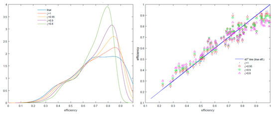
In the left panel of Figure 1, we report the true density of efficiency scores along with estimates of the density for $\zeta =1,$ 0.95, 0.98 and 0.9. The densities corresponding to different values of $\zeta$ are sample densities of posterior mean scores across the sample. In the right panel of Figure 1, we report 100 random efficiency scores corresponding to posteriors with different values of $\zeta$.

Figure 1. Artificial data, Model I.

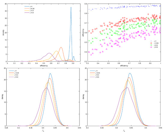
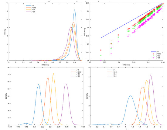
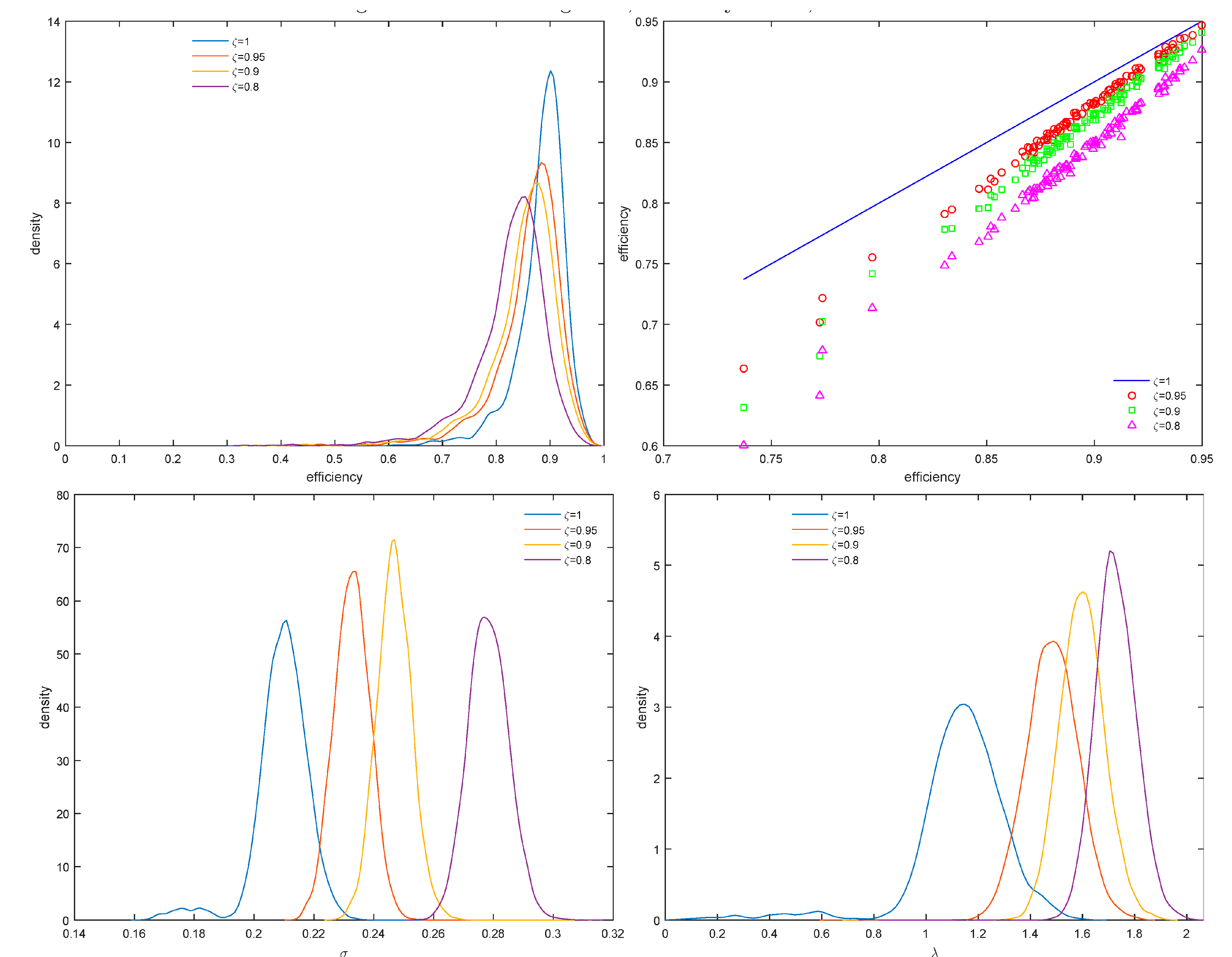
From the right panel of Figure 1, the differences between efficiency scores are not so marked as in Model II whose results are reported in the upper panels of Figure 2. In the lower panel, we report marginal posterior densities of the parameters ${\beta }_2$ and ${\beta }_3$. Efficiency scores are markedly different compared to $\zeta =1$ and as $\zeta$ decreases to 0.8 the efficiency distributions move to the left. The marginal posteriors of ${\beta }_2$ and ${\beta }_3$ also seem to be different although they are not far from the posterior mean when $\zeta =1$.

Figure 2. Artificial data, Model II.

4. Empirical Application

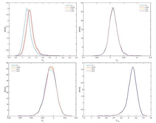
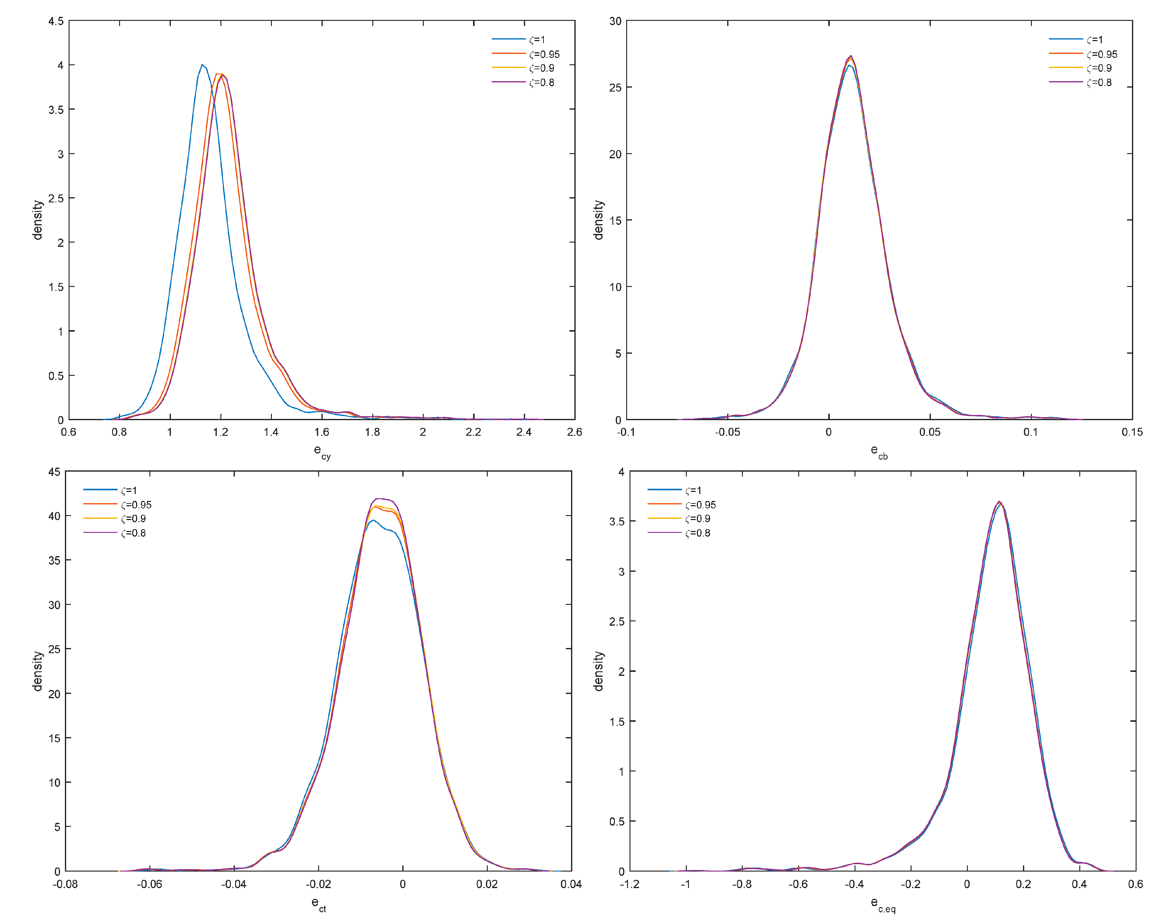
We use the banking data of Malikov et al. (2016) to estimate a translog cost frontier with five input prices, five outputs, a bad output (non-performing loans) and equity included as quasi-fixed input. The data is an unbalanced panel with 2397 bank-year observations for 285 large, relatively homogeneous US banks (2001:I–2010:IV). We refer the reader to Malikov et al. (2016) for further details on the data. Our results are reported in Figure 3 and Figure 4. As $\zeta$ increases, the distribution of efficiency scores shifts to the left, efficiency scores remain, however, highly correlated (upper right panel) and the posterior densities of both $\sigma$ and $\lambda$ shift to the right. Therefore, changes in distributional assumptions are likely to increase the variance of the error term but also the signal-to-noise ratio $\lambda$ from 1.2 to 1.8, on the average. From the results in Figure 4, posterior densities of output cost elasticity ($e_{cy}$), elasticity with respect to non-performing loans ($e_{cb}$), technical change ($e_{ct}$) and elasticity with respect to quasi-fixed equity ($e_{c,eq}$) remain robust as $\zeta$ changes, although this is less so for output cost elasticity and, therefore, returns to scale.

Figure 3. U.S Banking data, efficiency scores, $\sigma$ and $\lambda$.

Figure 4. U.S Banking data, elasticities.

Finally, to address the question of selecting $\zeta$, Miller and Dunson (2019) propose a measure of fit and a measure of model complexity. A measure of fit is given by the average log-likelihood and the complexity measure is given by the coarsened posterior. Instead, one case uses the log marginal likelihood:

$$ℳ\left(y,X\right)=\frac{p\left(\theta \right)p_{\zeta }(y|X,\theta )}{p_{\zeta }(\theta |y,X)} \forall \theta \in \mathsf{\Theta },$$

(18)

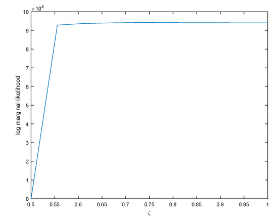
where $p_{\zeta }(y|X,\theta )$ is the tempered likelihood. Since this is an identity, we can use $\theta ={\overline{\theta }}_{\zeta }$, the posterior mean, and the denominator can be approximated with a multivariate normal distribution: $p_{\zeta }(\theta |y,X)\simeq {(2\pi )}^{-M/2}|V_{\zeta }{|}^{-1/2}$, where $V_{\zeta }=S^{-1}{\displaystyle \sum }_{s=1}^S({\theta }_{\zeta }^{\left(s\right)}-{\overline{\theta }}_{\zeta }){({\theta }_{\zeta }^{\left(s\right)}-{\overline{\theta }}_{\zeta })}^{\prime }$ is the posterior covariance matrix, and $M=dim\left(\theta \right)$. This is the Laplace approximation to log marginal likelihood (LML), see DiCiccio et al. (1997). We report the values of LML for ten values of $\zeta$ in Figure 5.

Figure 5. Normalized log marginal likelihood. Note: Log marginal likelihood is normalized so that its value at $\zeta =0.5$ is zero.

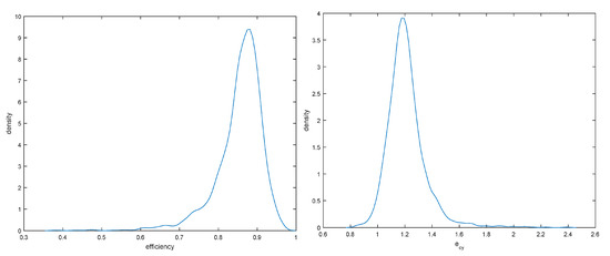
Since LML stabilizes at $\zeta =0.55$ one would be safe to average efficiency distributions over the different values of $\zeta$ shown in Figure 3. This is valid as alternative models (corresponding to different values of $\zeta$) have approximately the same posterior model probability given by: $p_{\zeta }\left(y,X\right)=\frac{{ℳ}_{\zeta }\left(y,X\right)}{{{\displaystyle \sum }}_{{\zeta }^{\prime }}{ℳ}_{{\zeta }^{\prime }}\left(y,X\right)}$. Moreover, from the upper right panel of Figure 4, these efficiency scores are highly correlated and slight changes in the data generating process affect only their location. Averaged efficiency densities and densities of output cost elasticity are presented in Figure 6.

Figure 6. Robust posteriors of efficiency and output cost elasticity.

The results indicate that efficiency ranges from 60% to slightly less than 100% with a median near 85%. As output cost elasticity averages 1.2, there seem to exist decreasing returns to scale in U.S large banks (the returns to scale measure is $1/e_{cy}$) with constant returns enjoyed by a sizable number of banks, and increasing returns being only exceptional. Finally, as model uncertainty increases (corresponding to lower values of $\zeta$), $e_{cy}$ increases slightly and its posterior shifts to the right (upper left panel of Figure 4).

Finally, in Table 1 we provide diagnostic measures to ensure that our MCMC draws provide access to the true posterior.

5. Concluding Remarks

We have proposed the concept of coarsened posteriors to robustify inferences from SFM. In an application to U.S banks, we find that economies of scale and technical change can be estimated in a relatively robust way, including elasticities with respect to equity and non-performing loans but efficiency inferences are less robust to the amount of data we use to robustify the posterior. This causes some concern as small changes in the distributional assumptions may change efficiency scores considerably. Fortunately, efficiency scores remain highly correlated across the robustness parameter ($\zeta$), at least in this application. In terms of future research, it would be interesting to examine the performance of robust posteriors in more complicated SFM and reconcile differences that arise from different approaches to modeling inefficiency. Moreover, an interesting avenue for future research would be based on recent work by Guo et al. (2018) who examined whether a parametric production frontier function is suitable in the analysis. Guo et al. (2018) developed two test statistics based on local smoothing and an empirical process, respectively and suggested also residual-based wild bootstrap versions of these two test statistics. As coarsening provides more robust results it is likely that the procedures in Guo et al. (2018) would tend to be in favor of the parametric specification although one has to resolve the issue of applying the Guo et al. (2018) procedures in a Bayesian context.

References

- DiCiccio, Thomas J., Robert E. Kass, Adrian Raftery, and Larr Wasserman. 1997. Computing Bayes factors by combining simulation and asymptotic approximations. Journal of the American Statistical Association 92: 903–15. [Google Scholar] [CrossRef]
- Feng, Guohua, Chuan Wang, and Xibin Zhang. 2019. Estimation of Inefficiency in Stochastic Frontier Models: A Bayesian Kernel Approach. Journal of Productivity Analysis 51: 1–19. [Google Scholar] [CrossRef] [Scilit]
- Fernández, Carmen, Jacek Osiewalski, and Mark F. J. Steel. 1997. On the use of panel data in stochastic frontier models with improper priors. Journal of Econometrics 79: 169–93. [Google Scholar] [CrossRef] [Scilit]
- Geweke, John F. 1992. Evaluating the Accuracy of Sampling Based Approaches to the Calculation of Posterior Moments. Bayesian Statistics 4. Edited by J. M. Bernardo, J. O. Berger, A. P. Dawid and A. F. M. Smith. Minneapolis: Federal Reserve Bank of Minneapolis, pp. 169–93. [Google Scholar]
- Greene, William H. 1999. Frontier Production Functions. In Handbook of Applied Econometrics. Volume II: Microeconomics. Edited by M. Hashem Pesaran and Peter Schmidt. Oxford: Blackwell, chp. 3. pp. 75–153. [Google Scholar]
- Guo, Xu, Gaorong Li, Michael John McAleer, and Wing-Keung Wong. 2018. Specification Testing of Production in a Stochastic Frontier Model. Sustainability 10: 3082. [Google Scholar] [CrossRef] [Scilit]
- Kumbhakar, Subal C., and C. A. Knox Lovell. 2000. Stochastic Frontier Analysis. Cambridge: Cambridge University Press. [Google Scholar]
- Malikov, Emir, Subal C. Kumbhakar, and Mike G. Tsionas. 2016. A cost system approach to the stochastic directional technology distance function with undesirable outputs: The case of U.S. banks in 2001–2010. Journal of Applied Econometrics 31: 1407–29. [Google Scholar] [CrossRef] [Scilit]
- Miller, Jeffrey W., and David B. Dunson. 2019. Robust Bayesian inference via coarsening. Journal of the American Statistical Association 114: 1113–25. [Google Scholar] [CrossRef] [Scilit]
- Parmeter, Christopher F., and Subal C. Kumbhakar. 2014. Efficiency Analysis: A Primer on Recent Advances. Foundations and Trends in Econometrics 7: 191–385. [Google Scholar] [CrossRef] [Scilit]