Abstract
This study examines the impact of changes in the yield curve factors on the Credit Default Swap (CDS) spreads of the U.S. industrial sectors. Stock returns and the crude oil-based volatility index are used in a quantile regression framework to test the validity of Merton’s model. The results suggest that the long-term factor of the yield curve is a negatively significant determinant of the CDS premia regardless of the sector and market state. The CDS spread of the financial sector exhibits sensitivity to the short-term factor of the yield rate in extreme market states. Basic materials, oil and gas and the utilities sector are responsive to variations in the medium-term factor of the yield rate in upmarket conditions. The empirical findings also suggest a significant inverse relationship between CDS spreads and stock returns.
JEL Classifications:
C22; E43; G12
1. Introduction
The analysis of the sensitivity of the credit default swap (CDS) premia to the yield rate has captured the renewed attention of researchers and market participants following the global financial crisis of 2008. According to the leading clearinghouses like ICE Trust and ICE Clear Europe, and CME Clearing, the CDS market exhibited resilience during the turbulent market conditions of 2008 (ICE 2010), making it even more relevant to economic and financial analysis. As a yield curve plots the interest rates of bonds of different maturities, which are known as the term of a debt for a given borrower in a given currency, it serves as a reliable determining factor of credit risk. The trade-off between the interest rate and credit risk is therefore certain, which implies that a rising interest rate could trigger the cost of investment and thereby necessitate a higher probability of default (Fofack 2005; Aver 2008; Louzis et al. 2012; Nkusu 2011). Advancement in the credit derivative market has led to the need for an in-depth analysis of the pricing of credit risk and its relationship, not only with a single yield rate but also its time-varying components, i.e., long-, short- and medium-term factors. Similarly, there is an extended need to observe the direction and magnitude of the relationship between the decomposed yield rate factors and the sector-wise CDS premia to uncover the price dynamics among the bond and the CDS markets, especially during the market crashes1 (Shi and Phillips 2017).
The yield curve sensitivity of any given firm represents the market risk of the firm, while the CDS spreads represent the credit risk of a firm (Bielecki and Rutkowski 2013). Therefore, through the study, an attempt has been made to examine the mixed effect of both risks on the ten U.S. industrial sectors. Most of the past studies have relied on the cross-sectional averaging across different entities/sectors over the long term to obtain any rational estimates of probabilities of default, as the occurrence of default events were considered rare. This study attempts to explore the interaction between the disintegrated yield curve factors and the sector-wise CDS premia by employing a quantile regression (QR) framework. QR is considered to be a preferred approach, as it can highlight any hidden sensitivities in the CDS spreads as a result of movements in the yield curve. One of the advantages of the QR framework is that unlike an OLS regression, it has robust results for any outliers (Cúrdia and Woodford 2015; Umar et al. 2018).
This research attempts to contribute to the existing literature on the determinants of CDS spreads in multiple ways. First, to check the validity of Merton’s model, three yield curve factors are used in a single econometric model. Second, a QR framework is employed to highlight the sensitivities between the yield rate factors and the CDS premia. Third, sector-wise CDS spreads are used to identify the heterogeneity in responses. Fourth, a sample period of 2007 to 2018 is used to include the global financial crisis period for analysis of the relationship between the variables in varying market states.
2. Literature Review
The motivation for this study stems from the multifaceted nature of the CDS market. Financial institutions such as banks and hedge funds mitigate their credit risk by actively engaging in the CDS market trading, which makes it a rapidly growing market. Along with this, the growth of the CDS market has led to a rise in the relevant empirical research due to easy access to the pricing data. The broadly classified dimensions of the empirical research are based on (1) the factors of credit default swap spreads, (2) the CDS market performance and (3) the correlation between the equity and CDS markets. The structural model of Merton (1974) and its expansions assert that leverage, asset volatility and market conditions such as interest rates serve as strong determinants of credit spreads (Tang and Yan 2010). Other major factors include firm-level elementary variables such as stock volatility, leverage, total asset size, profitability, cash ratios and investor risk aversion.
Several studies have concluded that CDS spreads display more favourable characteristics as a market indicator of distress. On the basis of rigorous empirical analysis, studies have found that CDS spreads tend to lead the signals derived from bond markets (Blanco et al. 2005). In addition, the evidence suggests that CDS trading tends to continue during periods of distress, in times when liquidity in bond markets may be severely restricted (Kiff et al. 2009). Credit risk modelling based on the correlation between interest rates and credit spreads has been the focus of research because of its significance in terms of implications. Most past research tends to establish a negative correlation between the short-term interest rate and credit spreads (Duffee 1998). In addition, quite often, a negative loading of the spot interest rate is included in a credit spread determination (Feldhütter and Lando 2008; Frühwirth et al. 2010; Driessen 2005). As the spot rates are determined by numerous risk factors, each factor could exhibit a different impact on credit spreads (Wu and Zhang 2008). On the other hand, interest rate factors with their different loadings (directly obtained from the term structure of LIBOR2/swap rates and CDS spreads) are common variables that determine the spot interest rate and credit.
Table 1 presents the major studies that have used various proxies for credit risk by considering different interest rates and their findings. In general, the findings reveal that the yield rate has a strong predictability power for the CDS premia, but the nature of the relationship between these variables remains inconclusive. Further, there is evidence that aggregate factors rather than firm-specific factors have significant explanatory power for the CDS spreads. Most of the past studies have used the conventional ordinary least squares (OLS) estimation and generalized autoregressive conditional heteroskedasticity (GARCH) framework to assess the nature of the relationship between CDS spreads and yield rates. In comparatively recent studies, Shahzad et al. (2017) has applied the Nonlinear Autoregressive Distributed Lag (NARDL) approach and Malhotra and Corelli (2018) used Granger causality to find the determinants of CDS spreads. However, none of these studies simultaneously used the yield curve factors in a single model to assess the impact of the small-, medium- and long-term yield rate shifts on the sector-wise CDS premia. Stock returns and an additional variable of the volatility index (OVX) are used as a proxy for the global macroeconomic financial risk in the analysis.

Table 1.
Studies on credit risk using credit default swap premia. CDS: credit default swap; OLS: ordinary least squares.
The motivation behind the study is to explore any sensitivities between the sector-wise CSD premia and the yield curve factors. The use of the single-yield rate in Merton’s model does not identify which of the factors of the yield rate is the most significant determinant in the pricing of the CDS spread for a given industrial sector. The simultaneous use of yield curve factors (i.e., the long-term (level), the short-term (slope) and the medium-term (curvature)) in place of the single-yield rate in Merton’s model is the contribution of this study. Besides this, it also attempts to explore the sensitivities between the sector-wise CSD premia and the yield curve factors in varying market states (bullish, bearish, normal), which would add to the strand of literature on the determinants of CDS premia.
3. Methodology
The modified adaptation of the Nelson–Siegel (1987) model, as suggested by Diebold and Li (2006), is used in the study. The empirical model of the analysis takes the following form:
where is sector-wise CDS spread; , and are the unanticipated movements in the level, slope and curvature factor of the yield curve; while , , and are the parameters that measure the sensitivity of CDS spreads to changes in the long-, medium- and short-term yield rates3. Diebold and Li (2006) used variations in the exponential component of the Nelson–Siegel model to obtain the factor structure of the yield curve, i.e., level, slope and curvature. Chen and Tzang (1988), Devaney (2001), Swanson et al. (2002) and Stevenson et al. (2007) used an array of interest rates jointly and established that regardless of the time structure, there exists a negative relationship between yield rates and CDS spreads. Zhu (2006) found that CDS spreads and bond yields may hold equivalence in the long run, but there is a substantial deviation in the short term. In addition, Shahzad et al. (2017) and (Malhotra) found that the equity prices and the volatility index serve as less significant but positive determinants of the industry-level CDS spreads. Wegener et al. (2017) suggested that positive oil price shocks lead to lower sovereign CDS. Thus, in the framework of the analysis, two potentially influential macroeconomic and financial variables are used, namely sector-wise returns and the OVX volatility index. Thus, the final proposed model can be specified as follows:
where and denote the changes in the sector-wise returns and volatility index.
The OLS regression model estimates the mean of the explained variable for specific values of the explanatory variables, i.e., it focuses on the central tendency of the variable and does not take into account the extreme values. In the case of non-normal errors, OLS regression fails to give robust results. Koenker and Bassett (1982) came up with the standard quantile regression (QR), which is an expansion of the classical linear regression model. It allows for the impact of an explanatory variable to vary across the quantiles of the explained variable. An additional attribute of this technique is that it aids in analysing the effect of independent variables not only in the middle of the distribution but also at the tails. In this way, it treats the outliers and non-normality issues. Therefore, it could be used to see how the relationships between variables are impacted in varying market states. Additionally, it acknowledges the implicit heterogeneity in the data by relaxing the assumption of independently and identically distributed error terms. Thus, in the case of non-normal errors, when the OLS regression fails to give robust results, the QR model proves to be efficient. Further, it is rational to assume that the impact of the yield curve factors on the sector-wise CDS premia may be disproportionate under specific market states (bearish/bullish). With this contextual intent, the quantile regression (QR) model is used to examine the sector-wise CDS spread sensitivities to changes in the yield curve factors. Eventually, in the QR framework, the multifactor model in Equation (2) can be rewritten as follows:
where denotes the conditional quantile of the CDS spreads for the sector-wise portfolios, 0 < θ < 1. The quantiles can be inferred to be signifying various market conditions. For instance, the upper quantiles are linked with an upbeat state of the market, while the lower quantiles are associated with a bearish state of the market. Conditional on the quantile, different weights are assigned to the positive and negative residuals, which are then minimized. The positive error terms carry a weight of θ, and the negative error terms are (1 − θ) in the objective function. For instance, at the 0.90 quantile, the positive error terms have a weight of 90, and the negative error terms have a weight of 10. At the 0.50 quantile, the weights are equal for the positive and negative error terms. The QR model allows for the parameters to vary over quantiles by amplifying θ from 0 to 1. In this way, a distribution of the explained variable contingent on the explanatory variables is obtained. Buchinsky (1995) advocated for the application of the bootstrap method to obtain the error terms of the QR coefficients, due to its improved results for smaller datasets.
4. Data and Results
4.1. Data Overview
The data series in the study consists of the CDS premia and the closing prices for the ten U.S. industrial sectors, the Standard & Poor’s 500 index and the OVX index (the CBOE Crude Oil Volatility Index4) over the period December 2007 to August 2018. The sample period (2007 to 2018) includes the global financial crisis period to study the relationship between the variables under varying market conditions.
The industrial sectors were categorized by following the Industry Classification Benchmark (ICB), namely “Oil and Gas”, “Basic Materials”, “Industrials”, “Consumer Goods”, “Consumer Services”, “Healthcare”, “Telecommunications”, “Utilities”, “Financials” and “Technology”. The CBOE Crude Oil ETF Volatility Index (OVX) quantifies the market’s expectation of 30-day volatility of crude oil prices by applying the VIX methodology to the United States Oil Fund. Recently, this index has gained wide acceptability in tracking and analyzing the volatility of oil futures. For the estimation of the level, slope and curvature factors of the yield curve, data on zero-coupon yields were obtained from the U.S. Treasury, ranging across 11 different maturities, i.e., for 1, 3 and 6 months and 1, 2, 3, 5, 7, 10, 20 and 30 years5. The first difference between two successive observations was taken to capture changes in the yield curve factors of level, slope and curvature. The sector-wise stock returns were computed as the first log difference between two consecutive observations. Further weekly data were used that comprised 2777 observations, as advocated by Ferrer et al. (2016), Flannery and James (1984) and Hirtle (1997), to take care of noisy data and irregularities such as non-random trading bias6. The data for the series were extracted from Thomson Financial DataStream and the U.S. Department of the Treasury.
The descriptive statistics for the entire sample are provided in Table 2. The weekly sector-wise mean returns are close to zero and mostly negative with a least value of −0.34 for the Consumer Services sector and a maximum value of 0.91 for the Healthcare sector. The negative mean returns indicate that over the sample period, these sectors faced financial losses or lacklustre returns. On a risk basis, measured by the standard deviation, the Utilities sector appears as the riskiest (52.8), with a minimum average weekly return of −680.2 and a maximum of 667.6. In contrast, with a minimum standard deviation, the Consumer Goods sector is the least risky (7.35). The majority of the sectors exhibit positive asymmetry, which implies that the returns are skewed to the right compared to a normal distribution. The kurtosis statistic exceeds the reference value of the normal distribution, i.e., 3, for all sectors, indicating that the data are leptokurtic. This suggests that the data are more peaked around the mean compared to the Gaussian distribution. Furthermore, the S&P 500 and OVX indices also reflect a negative trend with close to zero values and a standard deviation of 2.31 and 4.07, respectively. The S&P 500 data are negatively skewed (−1.17), while the OVX data are positively skewed (0.15). Both the data series are inherently leptokurtic. Finally, the mean weekly changes in the level, slope and curvature of the U.S. yield curve are positive but also close to zero, reflecting the rising trend. The factors of level and scope exhibit negative asymmetry (−0.01 and −1.23), while the curvature is positively skewed (0.93). The data of the three factors is also leptokurtic, like the rest of the series. Ultimately, for the entire series, the flight from normality is checked through the Jarque–Bera statistic, leading to rejection of the null hypothesis (normal distribution) at a 1% significance level. For the purpose of determining the order of integration of the data series, a unit root test and stationarity test results are provided in Table 3. The empirical statistics of the unit root tests (augmented Dickey–Fuller (ADF) and Phillips–Perron (PP)) and the stationarity test (Kwiatkowski–Phillips–Schmidt–Shin (KPSS)) results indicate stationarity for the data series of sector-wise returns, the S&P 500 index and variations in the level, slope and curvature of the yield curve. Contrary to this, the OVX series exhibited a unit root, so its first difference is used to ascertain stationarity. Further, Figure 1 presents the time trends in the U.S. sector-wise CDS premia, and Figure 2 presents the movements of the S&P 500 index, the OVX index and the level, slope and curvature of the yield curve.
Table 2.
Descriptive statistics of returns for the U.S. industrial sectors and risk variables.
Table 3.
Unit root tests of returns for the U.S. industrial sectors and risk variables.
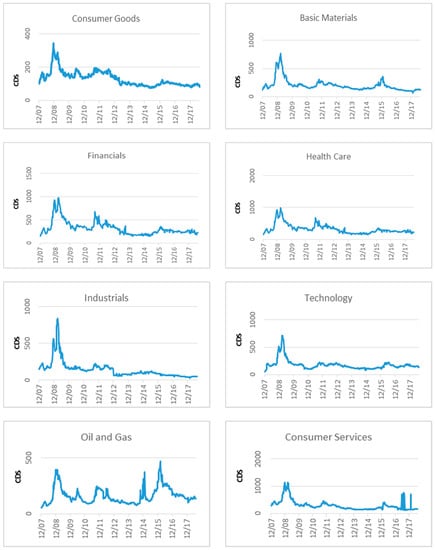
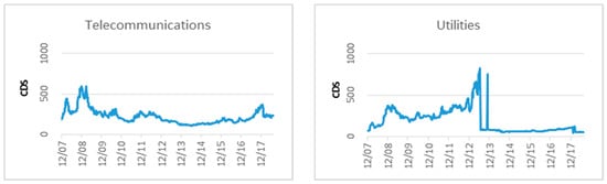
Figure 1.
Time trends of U.S. sector-wise weekly CDS spreads. Each panel represents one U.S. industrial sector and the relevant weekly CDS premia for the period December 2007 to August 2018.
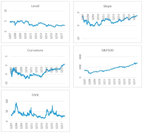
Figure 2.
Time trends of the U.S. weekly yield curve factors, market index S&P 500 and volatility index OVX for the period December 2007 to August 2018.
4.2. Empirical Results
The estimates of the QR model as detailed in Equation (3) are presented in this section. Table 4 reports the estimated coefficients of the U.S. yield curve factors at five quantiles (0:05; 0:25; 0:50; 0:75; 0:95) for the ten U.S. industrial sectors. For computing the standard errors of the coefficients, Buchinsky’s (1995) bootstrap method is used. The results show that the CDS premia are considerably sensitive to the fluctuations in the term structure of the yield curve. Particularly, the coefficients of changes in the level factor of the yield curve were negatively significant across the majority of the quantiles for most of the industrial sectors, except for in the lowest quantile (0.05). This implies that changes in the long-term factor of the yield rate serves as a highly significant determinant of the CDS premia, regardless of the sectors. This determining ability is held in all market conditions except for when it is bearish. Besides, the absolute value of the coefficients suggest that the CDS premia exhibit greater susceptibility to changes in the long-term factor of the yield curve, especially in the highest quantile (0.95), i.e., when the market is under extremely bullish conditions. In particular, the Basic Materials, Financials and Technology sectors display highest sensitivity to changes in the long-term yield rates, with estimated coefficient values of −39.3, −91.5 and −38.7 at a 1% level of significance in the upmarket conditions. The negative sign of the coefficients indicates an inverse relationship between the CDS premia and the yield curve factor. The CDS premia, in general, did not show signs of any unusual sensitivity to movements in the slope factor of the yield curve, except for in the Financial sector. This suggests that the Financial sector is exclusively responsive to changes in the short-term U.S. yield rates, specifically in the lowest quantile (0.05) and in the higher quantiles (0.75 and 0.95). In other words, the Financials sector is most influenced by fluctuations in the short-term interest rates under extremely bearish or bullish market conditions, with the magnitude being the highest in the booming market state (−76.02). The movements in the curvature factor of the yield curve cause responsiveness in the CDS prices of the Basic Materials, Oil and Gas and Utilities sectors. This indicates that the changes in the medium-term interest rates did not have a uniformly significant impact on all ten U.S. industrial sectors. The response of the sectors that showed significant sensitivity to these changes was more pronounced in the higher quantiles (0.75 and 0.95), highlighting the fact that during the bullish market conditions, these sectors show more sensitivity to shifts in the medium-term yield rates. Particularly the Oil and Gas sector and the Utilities sector exhibit significant sensitivity in both extremely bullish and bearish market situations (0.05, 0.75 and 0.95). The inverse relationship between yield rates and CDS spreads has also been evidenced by Alexander and Kaeck (2007), Chen et al. (2013) and Raunig (2015).
Table 4.
Quantile regression estimated yield rate coefficients of the U.S. industrial sectors.
The macroeconomic factors’ estimated coefficients, using the QR approach, are provided in Table 5. The results specify that the CDS premia are highly exposed to the changes in the S&P 500 index, regardless of the industrial sector. It is further observed that the vulnerability is at its lowest for the lowest quantile (0.05) for the majority of the sectors. This implies that changes in the market index is a key driver of changes in the CDS spreads in all market states, except for in bearish conditions. The negative coefficient signifies the inverse nature of the relationship between the CDS premia and the stock index. On the contrary, the sector-wise CDS premia show insensitivity to any changes in the OVX index. The sectors that display significant reactions are the Oil and Gas sector and Industrials, specifically in a bullish market state (0.95 quantile). These results are consistent with the empirical findings of Shahzad et al. (2017), which shows that the equity prices serve as a strong determinant of CDS spreads while oil prices do so to a lesser extent.
Table 5.
Quantile regression estimates of macroeconomic risk factors for U.S. industrial sectors.
Generalizing the findings, there is evidence that the long-term factor (level) of the yield rate is the most significant determinant in the pricing of the CDS spreads, regardless of the industrial sector. The inverse relationship is evidenced to be the strongest in the normal market state (mid-quantiles). The disproportionate response of the sector-wise CDS premia to any changes in the level, slope or curvature of the yield rate in various market states leads to the conclusion that some industrial sectors exhibit more sensitivity as compared to others. Further, by contrasting the OLS estimates, it is found that the QR approach provides a better illustration of the sector-wise CDS premia sensitivities subject to the market conditions.
5. Conclusions
This study attempted to explore the sensitivity of U.S. sector-wise CDS spreads to the yield rate factors. The motivation for this study stemmed from the multifaceted nature of the rapidly growing CDS market, in which participants such as banks and hedge funds actively trade credit risk. The increasing availability of pricing data has made the CDS market a growing area for empirical research. CDS and bond spreads provide for two complementary sources of information. In this context, the paper attempted to investigate the responsiveness of the U.S. sector-wise CDS premia to the variations in the term structure of the U.S. yield rates, market index and volatility index over the period of December 2007 to August 2018. Using yield rates of 11 different maturities and CDS spreads of 10 industrial sectors, the QR approach was employed to examine the sensitivities among the variables in specific market states. In conclusion, the long-term yield curve factor (slope) and the market index were evidenced to have been the fundamental factors explaining the variability in the CDS premia, especially in booming market conditions. This implies that the price of the derivatives incorporated macroeconomic shocks from the conventional stock markets, especially when investors believed that a stock or the overall market would go higher. These results are in line with the findings of Galil et al. (2014), Raunig (2015), Shahzad et al. (2017) and Malhotra and Corelli (2018), establishing that CDS premia are significantly influenced by macroeconomic variables. The findings of the study have important implications for various economic agents related to policy development and portfolio risk management through market busts and booms. The diversification benefits were greater when the economy was expanding, i.e., when the long-term yield rate (slope) increased (upper quantiles), especially for the financial sector. Financial institutions can also make hedging decisions based on these findings. Conversely, for most of the industrial sectors, there were limited diversification benefits when the market state was either bearish or normal (lower- or mid-quantiles), as then the changes in the yield curve factors (specifically slope and curvature) exhibited a weak relationship with CDS premia. In future research, more variables could be used by employing empirical approaches that further lead to an in-depth analysis of the nexus between CDS premia and yield rate factors. This study could be extended to other time series and regions. The findings can aid policy-makers and institutional investors in devising relevant policies for the development and restructuring of a derivative market by providing insight into the pricing dynamics of sector-wise CDS and yield rate fluctuations.
Funding
This research received no external funding.
Conflicts of Interest
The author declares no conflict of interest.
References
- Alexander, Carol, and Andreas Kaeck. 2007. Regime dependent determinants of credit default swap spread. Journal of Banking and Finance 32: 1008–21. [Google Scholar] [CrossRef]
- Aver, Boštjan. 2008. An empirical analysis of credit risk factors of the Slovenian banking system. Managing Global Transitions 6: 317–34. [Google Scholar]
- Baum, Christopher F., and Chi Wan. 2010. Macroeconomic uncertainty and credit default swap spreads. Applied Financial Economics 20: 1163–71. [Google Scholar] [CrossRef]
- Bielecki, Tomasz R., and Marek Rutkowski. 2013. Valuation and Hedging of OTC Contracts with Funding Costs, Collateralization and Counterparty Credit Risk. Working Paper. Chicago, IL, USA: Illinois Institute of Technology. [Google Scholar]
- Blanco, Roberto, Simon Brennan, and Ian W. Marsh. 2005. An Empirical Analysis of the Dynamic Relation between Investment-Grade Bonds and Credit Default Swaps. Journal of Finance 60: 2255–81. [Google Scholar] [CrossRef]
- Buchinsky, Moshe. 1995. Estimating the Asymptotic Covariance Matrix for Quantile Regression Models a Monte Carlo Study. Journal of Econometrics 68: 303–38. [Google Scholar] [CrossRef]
- Chen, K. C., and Daniel Tzang. 1988. Interest-rate sensitivity of real estate investment trusts. Journal of Real Estate Research 3: 13–22. [Google Scholar]
- Chen, Ren-Raw, Xiaolin Cheng, and Liuren Wu. 2013. Dynamic Interactions between Interest-Rate and Credit Risk: Theory and Evidence on the Credit Default Swap Term Structure. Review of Finance 1: 403–41. [Google Scholar] [CrossRef]
- Cúrdia, Vasco, and Michael Woodford. 2015. Credit Frictions and Optimal Monetary Policy (No. w21820). Cambridge: National Bureau of Economic Research. [Google Scholar]
- Devaney, Michael. 2001. Time-varying risk-premia for real estate investment trusts: A GARCH-M model. Quarterly Review of Economics and Finance 41: 335–46. [Google Scholar] [CrossRef]
- Diebold, Francis X., and Canlin Li. 2006. Forecasting the term structure of government bond yields. Journal of Econometrics 130: 337–64. [Google Scholar] [CrossRef]
- Driessen, Joost. 2005. Is default event risk priced in corporate bonds? Review of Financial Studies 18: 165–95. [Google Scholar] [CrossRef]
- Duffee, Gregory R. 1998. The relation between Treasury yields and corporate bond yield spreads. Journal of Finance 53: 2225–41. [Google Scholar] [CrossRef]
- Dufresne, Pierre Collin, Robert S. Goldstein, and J. Spencer Martin. 2001. The Determinants of Credit Spread Changes. Journal of Finance 56: 2177–207. [Google Scholar] [CrossRef]
- Düllmann, Klaus, and Agnieszka Sosinska. 2007. Credit default swap prices as risk indicators of listed German banks. Financial Markets and Portfolio Management 21: 269–92. [Google Scholar] [CrossRef]
- Ericsson, Jan, Kris Jacobs, and Rodolfo Oviedo. 2009. The determinants of credit default swap premia. Journal of Financial and Quantitative Analysis 44: 109–32. [Google Scholar] [CrossRef]
- Estrella, Arturo, and Gikas A. Hardouvelis. 1991. The term structure as a predictor of real economic activity. Journal of Finance 46: 555–76. [Google Scholar] [CrossRef]
- Fabozzi, Frank J., Lionel Martellini, and Philippe Priaulet. 2005. Predictability in the shape of the term structure of interest rates. Journal of Fixed Income 15: 40–53. [Google Scholar] [CrossRef]
- Fama, Eugene F. 1984. The information in the term structure. Journal of Financial Economics 13: 509–28. [Google Scholar] [CrossRef]
- Fama, Eugene, and Robert R. Bliss. 1987. The information in long-maturity forward rates. American Economic Review 77: 680–92. [Google Scholar]
- Feldhütter, Peter, and David Lando. 2008. Decomposing swap spreads. Journal of Financial Economics 88: 375–405. [Google Scholar] [CrossRef]
- Ferrer, Román, Vicente J. Bolós, and Rafael Benítez. 2016. Interest Rate Changes and Stock Returns: A European Multi-Country Study with Wavelets. International Review of Economics and Finance 44: 1–12. [Google Scholar] [CrossRef]
- Flannery, Mark J., and Christopher M. James. 1984. The Effect of Interest Rate Changes on the Common Stock Returns of Financial Institutions. Journal of Finance 39: 1141–53. [Google Scholar] [CrossRef]
- Fofack, Hippolyte L. 2005. Nonperforming Loans in Sub-Saharan Africa: Causal Analysis and Macroeconomic Implications. Working Paper Series 3769; Washington, DC: World Bank. [Google Scholar]
- Frühwirth, Manfred, Paul Schneider, and Leopold Sögner. 2010. The risk microstructure of corporate bonds: A case study from the German corporate bond market. European Financial Management 16: 658–85. [Google Scholar] [CrossRef]
- Galil, Koresh, Offer Moshe Shapir, Dan Amiram, and Uri Ben-Zion. 2014. The determinants of CDS spread. Journal of Banking & Finance 41: 271–82. [Google Scholar]
- Hirtle, Beverly J. 1997. Derivatives, Portfolio Composition, and Bank Holding Company Interest Rate Risk Exposure. Journal of Financial Services Research 12: 243–66. [Google Scholar] [CrossRef]
- ICE. 2010. Global Credit Derivatives Markets Overview: Evolution, Standardization and Clearing. Atlanta: Intercontinental Exchange, Inc. [Google Scholar]
- Kiff, John, Jennifer Elliott, Elias Kazarian, Jodi Scarlata, and Carolyne Spackman. 2009. Credit Derivatives: Systemic Risk and Policy Options. IMF Working Paper, WP/09/254. Washington, DC, USA: International Monetary Fund, November. [Google Scholar]
- Koenker, Roger, and Gilbert Bassett. 1982. Tests of Linear Hypotheses and L1 Estimation. Econometrica 50: 1577–83. [Google Scholar] [CrossRef]
- Louzis, Dimitrios P., Angelos T. Vouldis, and Vasilios L. Metaxas. 2012. Macroeconomic and bank-specific determinants of non-performing loans in Greece: A comparative study of mortgage, business and consumer loan portfolios. Journal of Banking & Finance 36: 1012–27. [Google Scholar]
- Malhotra, Jatin, and Angelo Corelli. 2018. The Determinants of CDS Spreads in Multiple Industry Sectors: A Comparison between the US and Europe. Risks 6: 89. [Google Scholar] [CrossRef]
- Merton, Robert C. 1974. On the pricing of corporate debt: The risk structure of interest rates. Journal of Finance 29: 449–70. [Google Scholar]
- Nelson, Charles R., and Andrew F. Siegel. 1987. Parsimonious modeling of yield curves. Journal of Business 60: 473–89. [Google Scholar] [CrossRef]
- Nkusu, Mwanza. 2011. Nonperforming Loans and Macro Financial Vulnerabilities in Advanced Economies. IMF Working Papers. Washington, DC, USA: International Monetary Fund, pp. 1–27. [Google Scholar]
- Raunig, B. 2015. Firm Credit Risk in Normal Times and during the Crisis: Are Banks less risky? Applied Economics 47: 2455–469. [Google Scholar] [CrossRef]
- Shahzad, Syed Jawad Hussain, Safwan Mohd Nor, Roman Ferrer, and Shawkat Hammoudeh. 2017. Asymmetric determinants of CDS spread: U.S. industry-level evidence through the NARDL approach. Economic Modelling 60: 211–30. [Google Scholar] [CrossRef]
- Shi, Shuping, and Peter C. B. Phillips. 2017. Detecting Financial Collapse and Ballooning Sovereign Risk. Oxford Bulletin of Economics and Statistics. [Google Scholar] [CrossRef]
- Stevenson, Simon, Patrick J. Wilson, and Ralf Zurbruegg. 2007. Assessing the time-varying interest rate sensitivity of real estate securities. European Journal of Finance 13: 705–15. [Google Scholar] [CrossRef]
- Swanson, Zane, John Theis, and K. Michael Casey. 2002. REIT risk premium sensitivity and interest rates. Journal of Real Estate Finance and Economics 24: 319–30. [Google Scholar] [CrossRef]
- Tang, Dragon Yongjun, and Hong Yan. 2010. Market conditions, default risk and credit spreads. Journal of Banking & Finance 34: 743–53. [Google Scholar]
- Umar, Zaghum, Syed Jawad Hussain Shahzad, Román Ferrer, and Francisco Jareño. 2018. Does Shariah compliance make interest rate sensitivity of Islamic equities lower? An industry level analysis under different market states. Applied Economics 50: 4500–21. [Google Scholar] [CrossRef]
- Wegener, Christoph, Tobias Basse, Frederik Kunze, and Hans-Jörg von Mettenheim. 2017. Oil prices and sovereign credit risk of oil producing countries: An empirical investigation. Quantitative Finance 16: 1961–68. [Google Scholar] [CrossRef]
- Wu, Liuren, and Frank Xiaoling Zhang. 2008. A no-arbitrage analysis of economic determinants of the credit spread term structure. Management Science 54: 1160–75. [Google Scholar] [CrossRef]
- Zhu, Haibin. 2006. An empirical comparison of credit spreads between the bond market and the Credit default swap market. Journal of Financial Service Research 29: 211–35. [Google Scholar] [CrossRef]
| 1 | See Shi and Phillips (2017). Detecting Financial Collapse and Ballooning Sovereign Risk, Oxford Bulletin of Economics and Statistics. |
| 2 | LIBOR, the London Interbank Offered Rate, is used as a basis for defining the lending rates in the international interbank market for the short-term loans. |
| 3 | Nelson and Siegel (1987) used an exponential components model based on three factors to capture the changes in the yield curve. Diebold and Li (2006) and Fabozzi et al. (2005) supported this model, as it is a good fit for the yield curve. |
| 4 | Chicago Board Options Exchange (CBOE) has created the implied volatility OVX that tracks the prices for the U.S. Oil Fund Exchange-traded fund while the volatility Index, VIX represents the market’s expectation of 30-day forward-looking volatility. |
| 5 | The dataset can be downloaded from https://www.treasury.gov/resource-center/data-chart-center/interest-rates/Pages/TextView.aspx?data=yield. |
| 6 | Ferrer et al. (2016), Flannery and James (1984) and Hirtle (1997) suggested the use of midweek data series to deal with the seasonality factor. |
© 2019 by the author. Licensee MDPI, Basel, Switzerland. This article is an open access article distributed under the terms and conditions of the Creative Commons Attribution (CC BY) license (http://creativecommons.org/licenses/by/4.0/).