Dealing with Low Interest Rates in Life Insurance: An Analysis of Additional Reserves in the German Life Insurance Industry

Abstract

Interest rates have been very low for several years, which is particularly challenging for life insurers. Since 2001, German life insurers have had to set an additional reserve due to low interest rates to ensure the protection of policyholders. However, the method introduced at that time to calculate these reserves was criticized, therefore, the German Federal Ministry of Finance replaced it with a new approach. In this article, we investigated the effects of the different methods on a typical German life insurer in various future interest rate scenarios and from various perspectives. For this purpose, we modelled such a life insurer holistically, considered its asset liability management and projected its future development in different interest rate scenarios using simulation techniques. Taking into account dependencies between assets, liabilities and interest rates, we analyzed and discussed our results from the life insurer’s, equity holders’, policyholders’ and regulators’ perspectives. The results show that the new method eliminated the weaknesses of the previous one and seems to be a suitable alternative to determine the additional reserve.

1. Introduction

For several years, interest rates have remained nearly at zero. This is especially challenging for life insurers, since they have many long-term contracts in their portfolios, with high guaranteed interest rates exceeding currently achievable interest rates. Due to the fact that local GAAP (generally accepted accounting principles) in Germany is a system with hidden assets in contrast to a market valuation, the actuarial reserves actually carefully calculated based on the actuarial interest rate determined at policy begin are in part inadequate, which is why there is the risk that promised guarantees cannot be met. In a system with market valuation on both sides of the balance scheme, the liabilities would already consider the current low interest rate environment reflected in higher market values of the obligations towards policyholders. To also consider the low interest rate environment with its implications on the actuarial reserves in German local GAAP and to ensure the protection of policyholders, since 2011, German life insurers have been required to provide an additional reserve due to low interest rates (“Zinszusatzreserve” or “ZZR”) that can be financed from the current surplus at the expense of, inter alia, profit participation. As described below in more detail, the ZZR is a step towards a more market-oriented valuation, taking into account the current interest rate environment but still considering the principles of a careful calculation in the German local GAAP. Since life insurance products with guarantees had been very popular in Germany, the low interest rate environment is particularly challenging for German life insurers. Some countries, such as Austria, have similar concepts (they are not the same due to different legal frameworks), while other countries, like France and Italy, do not intend to have such additional reserves.

Despite the fact that there seems to be agreement in Germany that the ZZR is necessary and useful, the method used to calculate the ZZR in Germany since 2011 has been under criticism. The German Actuarial Association (“DAV”) argued that the amount to be reserved increases very quickly in a very low interest rate environment. From 2011 to 2018, life insurers in Germany reserved in total nearly 60 billion EUR due to low interest rates (see Assekurata 2018), which was more than 6% of the total actuarial reserves (see GDV 2018); the share of the ZZR in the total actuarial reserves has risen sharply. If the interest rates stay comparably low or fall even further, the ZZR and its share in the total actuarial reserves will continue to rise (see Assekurata 2018; GDV 2018). To finance such a high ZZR, life insurers’ surplus may not be enough and they may have to realize their hidden assets, which implies that they must sell old high-yield securities (see DAV 2017)1. Besides causing transaction costs, life insurers are unable to find attractive investment opportunities when reinvesting this money (see DAV 2017). In particular, old high-yield securities are very important for life insurers in order to be able to meet their obligations towards policyholders in the future. Consequently, a fast rise in the ZZR may lead to problems for the insurers and threaten, instead of support, the protection of policyholders.

Moreover, even when the interest rates rise, there might be a time lag, meaning that despite increasing interest rates, it is likely that insurers still have to reserve more money (see DAV 2017). This is particularly challenging since hidden reserves on securities decrease when interest rates increase, implying that it might be difficult for life insurers to finance the rise of the ZZR, which could finally threaten their existence. Therefore, the DAV (2017) suggested a so-called corridor method, or Korridormethode, as an alternative. Recently, the German Federal Ministry of Finance followed this suggestion (see BMF 2018) and changed the calculation method of the ZZR.

One strand of the literature focuses on the effects of a low interest rate environment on life insurers in general (see, e.g., Berdin and Gründl 2015; Hieber et al. 2015; Holsboer 2000), while other literature investigates the risk management and value of guarantees in life insurance (see, e.g., Consiglio et al. 2001; Eckert et al. 2016; Eling and Holder 2013; Hieber et al. 2019; Kling et al. 2007b; Schmeiser and Wagner 2014). Further studies analyzed innovative product designs in life insurance, which rather avoid guaranteed interest rates (see, e.g., Alexandrova et al. 2017; Reuß et al. 2016; Wieland 2017). Finally, some papers (see, e.g., Albrecht 2015a; Albrecht and Weinmann 2015; Dalmis et al. 2013) focused on the impact of the ZZR (calculated using the old method) on German life insurers and Albrecht (2015b) compared the German case with Austria. However, to the best of our knowledge, no study investigated the effects of the different ZZR calculation methods on a life insurer. However, this is very relevant for life insurers (especially in Germany), policyholders, equity holders, politicians and regulators.

Thus, the aim of this paper was to investigate and discuss these methods from a holistic point of view, that is, from the perspective of a life insurer as well as their policyholders, equity holders and regulators. For this purpose, we modelled a typical German life insurer with a typical portfolio of policies and a standard asset allocation, taking into account their asset liability management. Using Monte Carlo simulation techniques, we simulated the life insurer’s future development for the next 10 years, depending on the ZZR calculation method, under various interest rate scenarios. This allowed us to study the effects of the two different ZZR calculation methods on certain key figures, such as the ZZR, the whole actuarial reserves, the development of hidden reserves, ruin probability and dividends, as well as surplus for policyholders. Only with a holistic model that considers the dependencies between assets and liabilities is it possible to analyze the full effects of both methods on the life insurer. Interpreting and discussing our results, we indeed found weaknesses in the old ZZR method, while the new corridor method managed to address these criticized points. As a result, the corridor method seems to provide a suitable solution in very low and in rising future interest rate scenarios.

This paper is structured as follows. Section 2, “Materials and Methods”, presents the old method to calculate the ZZR, as well as the new corridor method, and introduces our model framework. Section 3, “Results”, contains the calibration of the model life insurer and a resulting numerical analysis in different interest rate scenarios. Section 4, “Discussion”, summarizes and discusses implications.

2. Materials and Methods

2.1. Methods to Derive the ZZR Due to Low Interest Rates

2.1.1. Old Method of Calculating the ZZR in Germany (Valid from 2011–2018)

The old method of calculating the ZZR in Germany was legally based on § 341f para. 2 HGB (local GAAP) and § 5 paras. 3 and 4 DeckRV. § 341f para. 2 HGB stated that the actuarial reserve must consider interest rate obligations that can no longer be met by the current or expected returns. § 5 paras. 3 and 4 DeckRV then concretized how to calculate the expected return and described the measures to be taken if they are insufficient.

§ 5 para. 3 DeckRV required the calculation of a so-called reference interest rate (“Referenzzins”), denoted by $r_{ref,t}$ for year $t$, as the arithmetic mean over the last 10 years of yearly averages (rounded up to the second decimal place) of the zero-coupon Euro interest swap rates with a maturity of 10 years at the end of each month. These yearly averages are called basic interest rates (“Bezugszins”) and are denoted for year $t$ by $r_{bas,t}$. Hence, it is

$$r_{ref,t}=\frac{1}{10}·{{\displaystyle \sum }}_{j=0}^9{r}_{bas,t-j}.$$

Finally, following § 5 para. 4 DeckRV, for every contract, life insurers had to compare the current reference interest rate $r_{ref}$ with the highest relevant actuarial interest rate $r_{act}$. If $r_{ref}\ge r_{act}$, life insurers had to use $r_{act}$ to calculate the actuarial reserve. However, if $r_{ref}<r_{act}$, life insurers had to adjust the individual policy calculation of the actuarial reserves as follows: when calculating the present value, they had to use $\min (r_{ref},r_{act})$ for the next 15 years and $r_{act}$ for the time after the expiration of 15 years. Nevertheless, if using these specification results in a lower actuarial reserve for a contract than when using $r_{act}$, life insurers had to use $r_{act}$.

Consequently, for every contract, using this method leads to a higher or equal actuarial reserve than when always using $r_{act}.$ The difference between the actuarial reserve calculated in this manner and the actuarial reserve only calculated with $r_{act}$ is the additional reserve due to low interest rates, known as ZZR, which is not negative by definition.

2.1.2. New Corridor Method to Calculate the ZZR in Germany (Valid from 2018)

The DAV suggested to change the previously mentioned method and to use the corridor method (see DAV 2016). In the corridor method, the calculation of the reference interest rate is based on the reference interest rate $r_{ref,t}$ of the old method, but it is updated so that it can only move within a certain corridor from year to year, which implies an upper and a lower bound for each yearly new reference interest rate. As a result, this method limits the speed to build the ZZR.

Recently, the German Federal Ministry of Finance followed the suggestion of the DAV (see BMF 2018). Again, the calculation of the ZZR is legally based on § 341f para. 2 HGB (local GAAP) and § 5 DeckRV. However, § 5 DeckRV was updated as described below.

Let $r_{ref,t}$ denote the reference interest rate at the time $t$ calculated in the same manner as the old method (see Section 2.1) and ${\overline{r}}_{ref,t}$ represent the updated reference interest rate calculated using the new corridor method. Since the formulas depend on the calculation method used in the previous year, they would differ in the first year the corridor method is introduced. Consequently, we introduce an auxiliary variable $r_{aux,t-1}$, defined by

$$r_{aux,t-1}:=\{\begin{array}{l}{r}_{ref,t-1}, in the first year of the corridor method,\\ {\overline{r}}_{ref,t-1}, in the following years.\end{array}$$

Depending on the given percentage of deviation, denoted by $x=9\%$, the maximum deviation $maxdev\left(t\right)$ of the reference interest rate ${\overline{r}}_{ref,t}$ in year $t$ to the reference interest rate one year before $r_{aux,t-1}$ is defined by

$$maxdev\left(t\right):=x·\left|r_{bas,t}-r_{aux,t-1}\right|.$$

This implies for ${\overline{r}}_{ref,t}$ the following upper bound $upb\left(t\right)$ and lower bound $lob\left(t\right)$, respectively,

$$upb\left(t\right):=r_{aux,t-1}+maxdev\left(t\right)$$

and

$$lob\left(t\right):=r_{aux,t-1}-maxdev\left(t\right).$$

Since there are further conditions on the reference interest rate ${\overline{r}}_{ref,t}$, we first define ${\tilde{r}}_{ref,t}$ as

$${\tilde{r}}_{ref,t}:=\{\begin{array}{c}upb\left(t\right),\\ r_{ref,t},\\ lob\left(t\right),\end{array}\begin{array}{l}ifupb\left(t\right)<r_{ref,t},\hfill \\ iflob\left(t\right)\le r_{ref,t}\le upb\left(t\right),\hfill \\ if{r}_{ref,t}<lob\left(t\right).\hfill \end{array}$$

Even when interest rates rise, the reference interest rate in the old method might still drop, implying a higher ZZR due to the calculation as a 10-year arithmetic mean. To avoid this lag effect, the new method requires a comparison of the basic interest rate of the current year $r_{bas,t}$ with the reference interest rate of the last year $r_{aux,t-1}$. If $r_{bas,t}>r_{aux,t-1}$, the new method does not allow ${\overline{r}}_{ref,t}$ to be lower than $r_{aux,t-1}$ and vice versa, if $r_{bas,t}<r_{aux,t-1}$, it does not allow ${\overline{r}}_{ref,t}$ to be higher than $r_{aux,t-1}$. In this case the new method requires the use of the respective reference interest rate for the last year, i.e., ${\overline{r}}_{ref,t}=r_{aux,t-1}$.

Finally, the new reference interest rate in the corridor method is calculated by

$${\overline{r}}_{ref,t}:=\{\begin{array}{c}{r}_{aux,t-1}, if {\tilde{r}}_{ref,t}<{\overline{r}}_{ref,t-1}<r_{bas,t} or\\ if {\tilde{r}}_{ref,t}>{\overline{r}}_{ref,t-1}>r_{bas,t},\\ {\tilde{r}}_{ref,t}, otherwise.\end{array}$$

2.2. Model Framework

2.2.1. Overview

We followed Bohnert and Gatzert (2014) and considered a German life insurer with the simplified balance sheet at time $t$, given in

Table 1. Balance sheet of the life insurer at time t.

Assets	Liabilities
$A_t$	$E_t$
	$P{R}_t$
	$B_t$

.

$A_t$ denotes the book value of assets. The liability side comprises the book value of equity $E_t$, the book value of the policy reserves $P{R}_t$ and a buffer account $B_t$, which contains already generated surplus that is intended to be distributed to the policyholders via surplus distribution and to equity holders via dividend payments.

2.2.2. Asset and Liability Dynamics

In the following section, we described the asset and liability dynamics from $t$ to $t+1$.

Time t

At the balance sheet date $t$, the balance sheet is provided in Table 1. Additionally, we assumed, as in Eckert et al. (2016), that $A_t$ is divided into stocks and bonds.

$$A_t=A_t^B+A_t^S,$$

where $A_t^B$ is the book value of bonds and $A_t^S$ is the book value of stocks. The proportion of the book value of stocks to the book value of the total assets at time t is denoted by ${\beta }_t^S$, i.e.,

$${\beta }_t^S:=\frac{A_t^S}{A_t}.$$

Moreover, we denote with ${\tilde{A}}_t$ the market value of assets at time t and with ${\tilde{A}}_t^B$ and ${\tilde{A}}_t^S$ the corresponding market values of bonds and stocks. Therefore, the hidden assets $H{A}_t$ are given by $H{A}_t={\tilde{A}}_t-A_t$.

The policy reserves $P{R}_t$ at time $t$ consist of policy reserves for annuities $P{R}_t^A$ and for endowments $P{R}_t^E$, as in Bohnert et al. (2015), where $P{R}_t^A$ and $P{R}_t^E$ already comprise the respective current ZZR.

Additionally, we assumed, as in Bohnert et al. (2018), that the life insurer was already declared to withdraw $Sf{P}_{t^{+}}+D_{t^{+}}$ from the buffer $B_t$ immediately after the balance sheet date at time $t^{+}$. $Sf{P}_{t^{+}}$ is the surplus intended to be distributed to the policyholders and $D_{t^{+}}$ are the dividend payments to the equity holders.

Time$t^{+}$

Following Bohnert et al. (2018), we assume that at time $t^{+}$, i.e., immediately after the balance sheet date $t$, policyholders pay their annual premiums $P_{t^{+}}$, which already includes premiums for new business. The set of new policyholders is denoted by $N_{t^{+}}^A$ regarding annuities and $N_{t^{+}}^E$ regarding endowments. Furthermore, we assume that the life insurer pays the benefits $S_{t^{+}}$ to the policyholders2 and their share in surplus $Sf{P}_{t^{+}}$, as well as the dividends $D_{t^{+}}$ to the equity holders. Therefore, the current market value of assets at time $t^{+}$ is given by

$${\tilde{A}}_{t^{+}}={\tilde{A}}_t+P_{t^{+}}-S_{t^{+}}-Sf{P}_{t^{+}}-D_{t^{+}}.$$

Moreover, we assume that $P_{t^{+}}-S_{t^{+}}-Sf{P}_{t^{+}-}-D_{t^{+}}$ is invested according to the asset allocation between the stocks and bonds (book values) at the previous balance sheet date, which is why

$${\tilde{A}}_{t^{+}}^S={\tilde{A}}_t^S+{\beta }_t^S·\left(P_{t^{+}}-S_{t^{+}}-Sf{P}_{t^{+}}-D_{t^{+}}\right)$$

and

$${\tilde{A}}_{t^{+}}^B={\tilde{A}}_t^B+(1-{\beta }_t^B)·\left(P_{t^{+}}-S_{t^{+}}-Sf{P}_{t^{+}}-D_{t^{+}}\right).$$

The current (hypothetical) book value of assets at time is then, due to accounting standards, given by3

$$\begin{array}{c}{A}_{t^{+}}=A_t+\left(P_{t^{+}}-S_{t^{+}}-Sf{P}_{t^{+}}-D_{t^{+}}\right)·1_{\left(P_{t^{+}}-S_{t^{+}}-Sf{P}_{t^{+}}-D_{t^{+}}>0\right)}+\left(P_{t^{+}}-S_{t^{+}}-Sf{P}_{t^{+}}-D_{t^{+}}\right)\\ ·\left({\beta }_t^S·\frac{A_t^S}{{\tilde{A}}_t^S}+\left(1-{\beta }_t^S\right)·\frac{A_t^B}{{\tilde{A}}_t^B}\right)·1_{\left(P_{t^{+}}-S_{t^{+}}-Sf{P}_{t^{+}}-D_{t^{+}}<0\right)}\end{array}$$

with

$$\begin{array}{c}{A}_{t^{+}}^S=A_t^S+{\beta }_t^S·\left(P_{t^{+}}-S_{t^{+}}-Sf{P}_{t^{+}}-D_{t^{+}}\right)·1_{\left(P_{t^{+}}-S_{t^{+}}-Sf{P}_{t^{+}}-D_{t^{+}}>0\right)}+{\beta }_t^S·(P_{t^{+}}-S_{t^{+}}\\ -Sf{P}_{t^{+}}-D_{t^{+}})·\frac{A_t^S}{{\tilde{A}}_t^S}·1_{\left(P_{t^{+}}-S_{t^{+}}-Sf{P}_{t^{+}}-D_{t^{+}}<0\right)}\end{array}$$

and

$$\begin{array}{c}{A}_{t^{+}}^B=A_t^B+\left(1-{\beta }_t^S\right)·\left(P_{t^{+}}-S_{t^{+}}-Sf{P}_{t^{+}}-D_{t^{+}}\right)·1_{\left(P_{t^{+}}-S_{t^{+}}-Sf{P}_{t^{+}}-D_{t^{+}}>0\right)}+(1-\\ {\beta }_t^S)·\left(P_{t^{+}}-S_{t^{+}}-Sf{P}_{t^{+}}-D_{t^{+}}\right)·\frac{A_t^B}{{\tilde{A}}_t^B}·1_{\left(P_{t^{+}}-S_{t^{+}}-Sf{P}_{t^{+}}-D_{t^{+}}<0\right)}.\end{array}$$

Time${\left(t+1\right)}^{-}$

The market value of assets evolves between $t^{+}$ and ${\left(t+1\right)}^{-}$ from ${\tilde{A}}_{t^{+}}$ to ${\tilde{A}}_{{\left(t+1\right)}^{-}}$, where we model the dynamics of the stock and the bonds separately.

In accordance with Bohnert et al. (2013) and Bohnert et al. (2018), we assume that the market value of stocks follows a geometric Brownian motion, which, for an investment $I_t$, is given by

$$d{I}_t=\mu ·I_t·dt+\sigma ·I_t·d{W}_t^P,$$

where $\mu$ is the drift, $\sigma$ the volatility and $W^P$ a standard Brownian motion on the probability space $\left(\mathsf{\Omega },\mathsf{\Phi },P\right)$, with the filtration $\mathsf{\Phi }$ generated by the Brownian motion and the real-world measure $P$.

The solution to this stochastic differential equation is given by

$$I_{t+1}=I_t·\exp \left(\mu -\frac{{\sigma }^2}{2}+\sigma ·\left(W_{t+1}^P-W_t^P\right)\right),$$

which is why the one-period return (continuous) is normally distributed with mean $m=\mu -\frac{{\sigma }^2}{2}$ and volatility $\sigma$.

As a result, in our case, the market value of the stocks ${\tilde{A}}_{{\left(t+1\right)}^{-}}^S$ at time ${\left(t+1\right)}^{-}$ based on ${\tilde{A}}_{t^{+}}^S$ is given by

$${\tilde{A}}_{{\left(t+1\right)}^{-}}^S={\tilde{A}}_{t^{+}}^S·\frac{I_{t+1}}{I_t}.$$

To simplify, we assume that the life insurer has only zero-coupon bonds in their portfolio, which have different maturity dates and par values. Given the par value $Pa{r}_j$ and time to maturity $M_j$, the present value $P{V}_j$ of the zero-coupon bond $j$ is given by

$$P{V}_j=\frac{Pa{r}_j}{{\left(1+i\right)}^{M_j}},$$

where $i$ is the current corresponding market interest rate. In our model, $i$ depends on the respective interest rate scenario considered in the next section; ${\tilde{A}}_{{\left(t+1\right)}^{-}}^B$ is then given as the sum of the present values of all zero-coupon bonds in the life insurer’s portfolio.

For pricing and reserving, we used mortality tables from the DAV, i.e., “DAV 2004 R” for annuities and “DAV 2008 T” for endowments. These mortality tables are first-order mortalities including a safety loading. Therefore, to more realistically model the deaths in the time between $t^{+}$ and ${\left(t+1\right)}^{-}$, we followed Bohnert et al. (2015) and used the aforementioned tables’ underlying best estimates, which are second-order mortalities without safety loadings. We then denoted the set of policyholders that died between $t$ and $t+1$ by $T_{t+1}^A$ if they had annuities and $T_{t+1}^E$ if they had endowments.

The life insurer then has to make the lump sum payment on death to endowment holders as in Bohnert et al. (2015), denoted by $S_{{\left(t+1\right)}^{-}}$, which implies a reduction of $S_{{\left(t+1\right)}^{-}}$ of the market value of assets ${\tilde{A}}_{{\left(t+1\right)}^{-}}$ with the effects on the corresponding book value of assets, as mentioned above. Here, we assume that the life insurer reduces stocks and bonds in the same way as before.

To calculate the policy reserves at ${\left(t+1\right)}^{-}$ including ZZR, we first calculated the new reference interest rates $r_{ref,t+1}$ and ${\overline{r}}_{ref,t+1}$, depending on the chosen ZZR-method and the respective interest rate scenario.

The policy reserve is then given as the sum of the policy reserves of all annuities $P{R}_{{\left(t+1\right)}^{-}}^A$ and endowments $P{R}_{{\left(t+1\right)}^{-}}^E$ in the current portfolio of the life insurer, i.e., without the policies of the policyholders who have already died. Thus, following Bohnert et al. (2015), the total policy reserve $P{R}_{{\left(t+1\right)}^{-}}$ is given by

$$P{R}_{{\left(t+1\right)}^{-}}=P{R}_{{\left(t+1\right)}^{-}}^A+P{R}_{{\left(t+1\right)}^{-}}^E={\displaystyle \sum }_{i\in (P{H}_t^A\cup N_{t^{+}}^A)\backslash T_{t+1}^A}{}_{m_i}V_{x_i}^{A,ZZR}+{\displaystyle \sum }_{j\in (P{H}_t^E\cup N_{t^{+}}^E)\backslash T_{t+1}^E}{}_{m_j}V_{x_j}^{E,ZZR},$$

where $P{H}_t^A$ and $P{H}_t^E$ are the set of policyholders of annuities and endowments at the balance sheet date $t$, and ${}_{m_i}V_{x_i}^{A,ZZR}$ and ${}_{m_j}V_{x_j}^{E,ZZR}$ denote the actuarial reserve for an individual annuity and endowment including ZZR. Here, $x_i$ and $x_j$ denote the age of policyholders $i$ and $j$ at the beginning of the contract and $m_i$ and $m_j$ represent the time between the beginning of the contract and now.

For the sake of simplicity, we assume that the life insurer sells only annuities with pension payments starting immediately. The actuarial reserve without ZZR ${}_{m}V_x^A$ for an at policy begin x-year old person after m years with yearly annuity payments $R$ is given by

$${}_{m}V_x^A=R·{\mathsf{ä}}_{x+m}.$$

(1)

However, as described in the previous section, calculating the ZZR requires using the minimum of the reference interest rate and the actuarial interest rate instead of the actuarial interest rate for discounting cashflows that occur over the next 15 years. Therefore, Equation (1) must be adjusted. Since mortality tables calculate a maximum age $\omega$, it is possible that the annuity could expire within the next 15 years. Consequently, we must distinguish between two cases.

$${}_{m}V_x^{A,ZZR}=\{\begin{array}{c}R·\left({\mathsf{ä}}_{x+m:\overline{15}|}^{ref}+{\left(\frac{1}{1+r_{ref}}\right)}^{15}·{}_{15}p_{x+m}·{\mathsf{ä}}_{x+m+15}\right), if x+m+15<\omega ,\\ R·{\mathsf{ä}}_{x+m}^{ref}, else.\end{array}$$

The superscript $ref$ in the present values means that these cashflows are discounted using the current reference interest rate; no superscript means the standard actuarial interest rate is used. Note that the reference interest rate differs when using the old or the new corridor method to calculate the ZZR.

In terms of endowment policies, for the sake of simplicity we assume that policyholders pay a single premium at the beginning of the contract instead of annual premiums. The actuarial reserve without ZZR ${}_{m}V_x^E$ for an at policy begin x-year old person after m years with a guaranteed lump sum payment $S$ on maturity in $n$ years or on death is given by

$${}_{m}V_x^E=S·A_{x+m:\overline{n-m|}}.$$

(2)

Taking into account the ZZR, we again have to adjust the calculation without the ZZR given in (2). Letting the superscript $ref$ denote that cashflows are discounted using the current reference interest rate (depending on the ZZR calculation method) and allowing no superscript to mean that cashflows are discounted using the standard actuarial interest rate, we get

$${}_{m}V_x^{E,ZZR}=\{\begin{array}{c}S·\left({}_{|15}A_{x+m}^{ref}+{}_{15}{}^{}E_{x+m}^{ref}·A_{x+m+15:\overline{n-m-15}|}\right), if n-m>15,\\ S·A_{x+m:\overline{n-m|}}^{ref}, else.\end{array}$$

Just before the next balance sheet date $t+1$, we aim to model the management decisions of the life insurer regarding the realization of hidden reserves, deposits from the surplus in the buffer and withdrawals from the buffer in the next period (dividends and surplus for policyholders).

Therefore, we calculate the current (hypothetical) book value of assets $A_{{\left(t+1\right)}^{-}}$, which, due to accounting standards, is given by

$$A_{{\left(t+1\right)}^{-}}=\min \left(A_{t^{+}}^S,{\tilde{A}}_{{\left(t+1\right)}^{-}}^S\right)+\min \left(A_{t^{+}}^B,{\tilde{A}}_{{\left(t+1\right)}^{-}}^B\right).$$

Following Kling et al. (2007a, 2007b), we assume that the book value of equity $E_t$ is constant over time except if the life insurer gets into a critical situation. Moreover, we assume that the life insurer aims to pay at least constant over time dividends D or dividends higher than this constant value, i.e., $D_{{\left(t+1\right)}^{+}}\ge D,\forall t$, since equity holders demand a certain return.

Furthermore, we assume, as in Bohnert et al. (2018), that the life insurer aims to declare deposits from the surplus in the buffer $Sf{B}_{{\left(t+1\right)}^{-}}$, as well as withdrawals from the buffer, indicating a surplus for policyholders for the next period $Sf{P}_{{\left(t+1\right)}^{+}}$ that are also at least constant over time or higher than this constant value, i.e., $Sf{B}_{{\left(t+1\right)}^{-}}\ge SfB,\forall t$ and $Sf{P}_{{\left(t+1\right)}^{+}}\ge SfP,\forall t$. The reason is that the buffer and the withdrawals from the buffer (dividends and surplus for policyholders) influence the reputation of the insurer and its attractiveness for possible new business.

The aforementioned goals of the life insurer must be financed by its surplus. Surplus is generated since the mortality rates used to calculate the policy reserves have safety loadings, compared to the more realistic mortality probabilities. Moreover, surplus is generated due to the return on the assets that exceeds the required return for the liabilities (including ZZR). Here, we must consider that the life insurer can influence this part of the gross surplus within certain limits due to possible realizations of hidden reserves, which are given by $H{R}_{{\left(t+1\right)}^{-}}={\tilde{A}}_{{\left(t+1\right)}^{-}}-A_{{\left(t+1\right)}^{-}}$. Due to accounting standards, the book value of assets does not necessarily increase when the market value increases. Consequently, if market values increase but the life insurer does not sell assets, this does not generate surplus; only the hidden reserves on the assets increase. Selling assets and reinvesting them, however, decreases the hidden reserves but increases the book value of assets and therefore generates surplus. On the other hand, this implies possibly selling high-yield bonds and buying bonds with lower coupons, which weakens the substance of the life insurer by decreasing its buffer off hidden assets.

To model the management decision with respect to selling assets and reinvesting them, we first calculate the gross surplus $G{S}_{{\left(t+1\right)}^{-}}$ at ${\left(t+1\right)}^{-}$ without realizing additional hidden reserves, dividends and surplus distribution, i.e.,

$$G{S}_{{\left(t+1\right)}^{-}}:=A_{{\left(t+1\right)}^{-}}-P{R}_{{\left(t+1\right)}^{-}}-E_t-\left(B_t-D_{t^{+}}-Sf{P}_{t^{+}}\right).$$

If $G{S}_{{\left(t+1\right)}^{-}}$ is already enough to finance the aforementioned assumptions, i.e.,

$$G{S}_{{\left(t+1\right)}^{-}}\ge D+SfP\left(=:SfB\right),$$

(3)

we assume that the life insurer does not realize any hidden reserves, since it is not necessary and would weaken its substance. If the left side in (3) is strictly greater, we assume that the life insurer deposits more money in the buffer during this period and withdraws accordingly more money in the next period to let the policyholders and equity holders participate in this surplus.

However, if the inequality (3) is not satisfied, i.e.,

$$G{S}_{{\left(t+1\right)}^{-}}<SfB,$$

we assume that the life insurer realizes hidden reserves, increasing $A_{{\left(t+1\right)}^{-}}$ so that $G{S}_{{\left(t+1\right)}^{-}}$ increases for as long as

$$G{S}_{{\left(t+1\right)}^{-}}=SfB,$$

(4)

so that the life insurer can pay the policyholders and equity holders the intended dividends and surplus benefits in the next period.

However, if the hidden reserves are not sufficient to obtain the equality in (4), the life insurer faces a critical situation. As a result, the life insurer reduces the deposit in the buffer, the dividend payments and the surplus benefit for the policyholders as follows:

Instead of $D$, the dividend payments in the next period are only

$$D_{{\left(t+1\right)}^{+}}=G{S}_{{\left(t+1\right)}^{-}}·\frac{D}{D+SfP},$$

and the surplus benefit for the policyholders instead of $SfP$ is accordingly

$$Sf{P}_{{\left(t+1\right)}^{+}}=G{S}_{{\left(t+1\right)}^{-}}·\frac{SfP}{D+SfP},$$

where $G{S}_{{\left(t+1\right)}^{-}}$ is the gross surplus after realizing all of the life insurers hidden reserves.

Therefore, the deposit in the buffer $Sf{B}_{{\left(t+1\right)}^{-}}=D_{{\left(t+1\right)}^{+}}+Sf{P}_{{\left(t+1\right)}^{+}}$ is lower.

If, after realizing all hidden reserves, we still have $G{S}_{{\left(t+1\right)}^{-}}<0$, the life insurer is allowed to use the remaining money from the buffer in this critical situation, i.e., $B_t-D_{t^{+}}-Sf{P}_{t^{+}}$ to strengthen their equity. However, if

$$G{S}_{{\left(t+1\right)}^{-}}+E_t+B_t-D_{t^{+}}-Sf{P}_{t^{+}}<0,$$

then the life insurer is insolvent.

Time$t+1$

Based on the balance sheet of the previous balance sheet date and the dynamics and decisions mentioned above, we finally obtain the balance sheet at time $t+1$, which is given in

Table 2. Balance sheet of the life insurer at time $t+1$.

Assets	Liabilities
$A_{t+1}$	$E_{t+1}$
	$P{R}_{t+1}$
	$B_{t+1}$

.

3. Results

3.1. Input Parameters and Interest Rate Scenarios

3.1.1. Input Parameters

We started at the balance sheet date 31 December 2017 and denoted this date for ease of notation by $t=0$. Based on statistics regarding the asset allocations of German life insurers provided by Assekurata (2016), we assumed that, at this time, the book value of assets of the life insurer was 50 billion EUR with a market value of 60 billion EUR. Following Assekurata (2016), the majority was invested in bonds (book value 47.5 billion EUR, market value 57 billion EUR) and the minority in stocks (book value 2.5 billion EUR, market value 3 billion EUR). Therefore, we had a proportion of stocks of ${\beta }_0^S=5\%$. Considering the monthly performance of the German stock market index DAX between January 2005 and December 2017 to calibrate the stock dynamics, this led to one-year stock returns of 10.45% on average and a corresponding volatility of 19.54%. According to Assekurata (2016), the average duration of bonds in the portfolio of a life insurer is approximately 10 years. Since in our model the life insurer only had zero-coupon bonds with duration equaling their time to maturity, we assumed that the life insurer holds a portfolio of zero-coupon bonds with an average time to maturity of 10 years. More precisely, we assumed that the life insurer’s investment was evenly distributed (with respect to book value and market value of the bonds) on zero-coupon bonds with time to maturity of 5, 10 and 15 years. To keep the insurer’s duration approximately at 10 years over time, when reinvesting money in the following years, the life insurer invested in zero-coupon bonds with a maturity of 15 years, which were priced based on the interest rate of the respective interest rate scenario. Thus, the interest rate scenarios determined their future dynamics.

Following Eckert et al. (2016), the equity $E_0$ was $1\%$ of the total assets, i.e., $E_0=500$ million EUR. Moreover, based on empirical data from Assekurata (2016), we assumed that $B_0=3$ billion EUR, with $D_{0^{+}}=D=50$ million EUR and $Sf{P}_{0^{+}}=SfP=500$ million EUR.

Since total assets equal total liabilities, policy reserves were $P{R}_0=46.5$ billion EUR. Based on statistics from Assekurata (2017), we assumed that $P{R}_0^A=26.5$ billion EUR and $P{R}_0^E=20$ billion EUR. Regarding pricing and reserving, we used mortality tables from the DAV, i.e., “DAV 2004 R” for annuities and “DAV 2008 T” for endowments, which use a maximum age of 121. For the sake of simplicity, we assumed that each annuity was sold to a 70-year-old person, starting immediately with annuity payments of 2000 EUR until the policyholder dies. With regard to endowments, we assumed that each endowment holder was 25 years old at the start of the policy and the time to maturity was 45 years, with a lump sum payment of 50,000 EUR.

Due to the regulatory requirements, the actuarial interest rate used to calculate annuities and endowments in Germany changes over time. However, the ZZR depends on the actuarial interest rate, which is why we assumed that our life insurer had policies with different actuarial interest rates and policy begins in their portfolio. The proportion of the actuarial reserve of each policy generation of the total actuarial reserve was calibrated based on data from Assekurata (2017). The resulting input parameters for the portfolios of annuities and endowments are given in

Table 3. Annuities in the portfolio.

Start Date (01/01)	Actuarial Interest Rate in %	Annual Annuity Payment in Million EUR	Actuarial Reserve (Excl. ZZR) at t = 0 in Million EUR	ZZR at $\mathit{t}=0$ $({\mathit{r}}_{\mathit{r}\mathit{e}\mathit{f},0}=2.21\mathit{\%})$ in Million EUR
1986	3.00	143.36	834.75	25.89
1994	3.50	599.41	4348.65	262.12
2000	4.00	600.85	5514.65	525.99
2003	3.25	302.39	3185.30	200.51
2006	2.75	322.05	3884.90	142.49
2011	2.25	289.13	4282.40	136.64
2014	1.75	151.67	2615.55	0
2016	1.25	62.54	1219.00	0
2017	0.90	29.26	614.80	0

and

Table 4. Endowments in the portfolio.

Start Date (01/01)	Actuarial Interest Rate in %	Lump sum Payment in Million EUR	Actuarial Reserve (Excl. ZZR) at t = 0 in Million EUR	ZZR at $\mathit{t}=0$ $({\mathit{r}}_{\mathit{r}\mathit{e}\mathit{f},0}=2.21\mathit{\%})$ in Million EUR
1986	3.00	819.56	630.00	55.32
1994	3.50	5321.17	3282.00	532.64
2000	4.00	8526.75	4162.00	918.83
2003	3.25	5012.82	2404.00	329.22
2006	2.75	6211.13	2932.00	218.16
2011	2.25	7064.13	3232.00	18.65
2014	1.75	3842.03	1974.00	0
2016	1.25	1519.91	920.00	0
2017	0.90	672.66	464.00	0

, respectively. To simplify, we assumed that the annuities of one policy generation were sold on one date.

Since we simulated the next 10 years, we assumed that new business every year was constant and the same as in 2017. Therefore, we assumed that every year the life insurer sold 14,631 immediately starting annuities to 70-year-old persons, with an annual annuity payment of 29.26 million EUR in total and 13,454 endowment policies to 25-year-old persons with time to maturity 45 years and a lump sum payment in total of 672.70 million EUR on maturity or on death. For pricing, we used the current actuarial interest rate of 0.90%.

3.1.2. Interest Rate Scenarios

The basic interest rate at the end of 2017 $r_{bas,0}$ was 0.90% and the corresponding reference interst rate $r_{ref,0}$ was 2.21%. Starting at the end of 2017, we considered, in our simulation, four different interest rate scenarios, which are given in

Table 5. Overview of interest rate scenarios for the basic interest rate $r_{bas,t}$.

Scenario	2018	2019	2020	2021	2022	2023	2024	2025	2026	2027
	$\left(\mathit{t}=1\right)$	$\left(\mathit{t}=2\right)$	$\left(\mathit{t}=3\right)$	$\left(\mathit{t}=4\right)$	$\left(\mathit{t}=5\right)$	$\left(\mathit{t}=6\right)$	$\left(\mathit{t}=7\right)$	$\left(\mathit{t}=8\right)$	$\left(\mathit{t}=9\right)$	$\left(\mathit{t}=10\right)$
1	0.90%	0.90%	0.90%	0.90%	0.90%	0.90%	0.90%	0.90%	0.90%	0.90%
2	0.60%	0.30%	0.00%	0.00%	0.00%	0.00%	0.00%	0.00%	0.00%	0.00%
3	1.11%	1.32%	1.53%	1.74%	1.95%	2.16%	2.37%	2.58%	2.79%	3.00%
4	1.60%	2.30%	3.00%	0.50%	0.50%	0.50%	0.50%	0.50%	0.50%	0.50%

. In each scenario we made assumptions about the basic interest rate for the next 10 years. Based on this, we then calculated the respective reference interest rate of the old and the new corridor methods in each scenario. Using these interest rates, in the next subsection we simulated the future dynamics of the life insurer from 2018 to 2027. Note that we followed the German Federal Ministry of Finance (see BMF 2018) and assumed that $x=9\%$ in our base case, while we also conducted sensitivity analyses for different values of $x$.

We aimed to cover all the relevant future interest rate scenarios. In Scenario 1, we assumed that the basic interest rate from 2017 (0.90%) remained the same until 2027. Scenario 2 considered a situation in which the basic interest rate fell from 0.90% in 2017 evenly to 0.00% in 2020 and remained there until 2027. Scenario 3, however, focused on a situation in which interest rates increased evenly from 0.90% in 2017 to 3.00% in 2027. Finally, in Scenario 4, we assumed that interest rates first increased evenly to 3.00% until 2020 and then plummeted immediately to 0.50% in 2021, where they remained until 2027. Hence, we considered interest rate scenarios of constant, rising and falling interest rates, as well as a mixture of a rising, then falling and then constant interest rate scenario.

3.2. The Impact of the ZZR Method on the Life Insurer under Various Interest Rate Scenarios

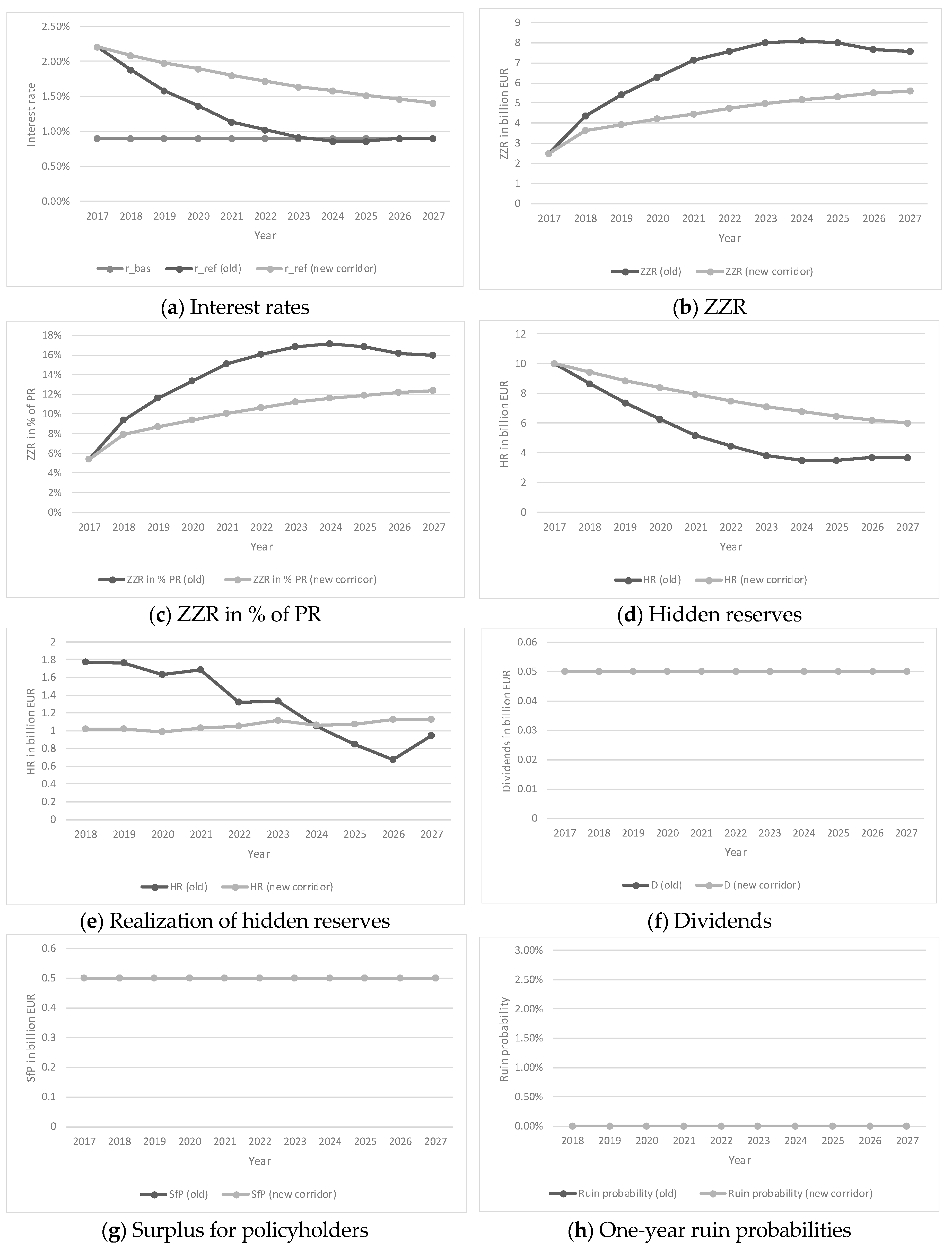
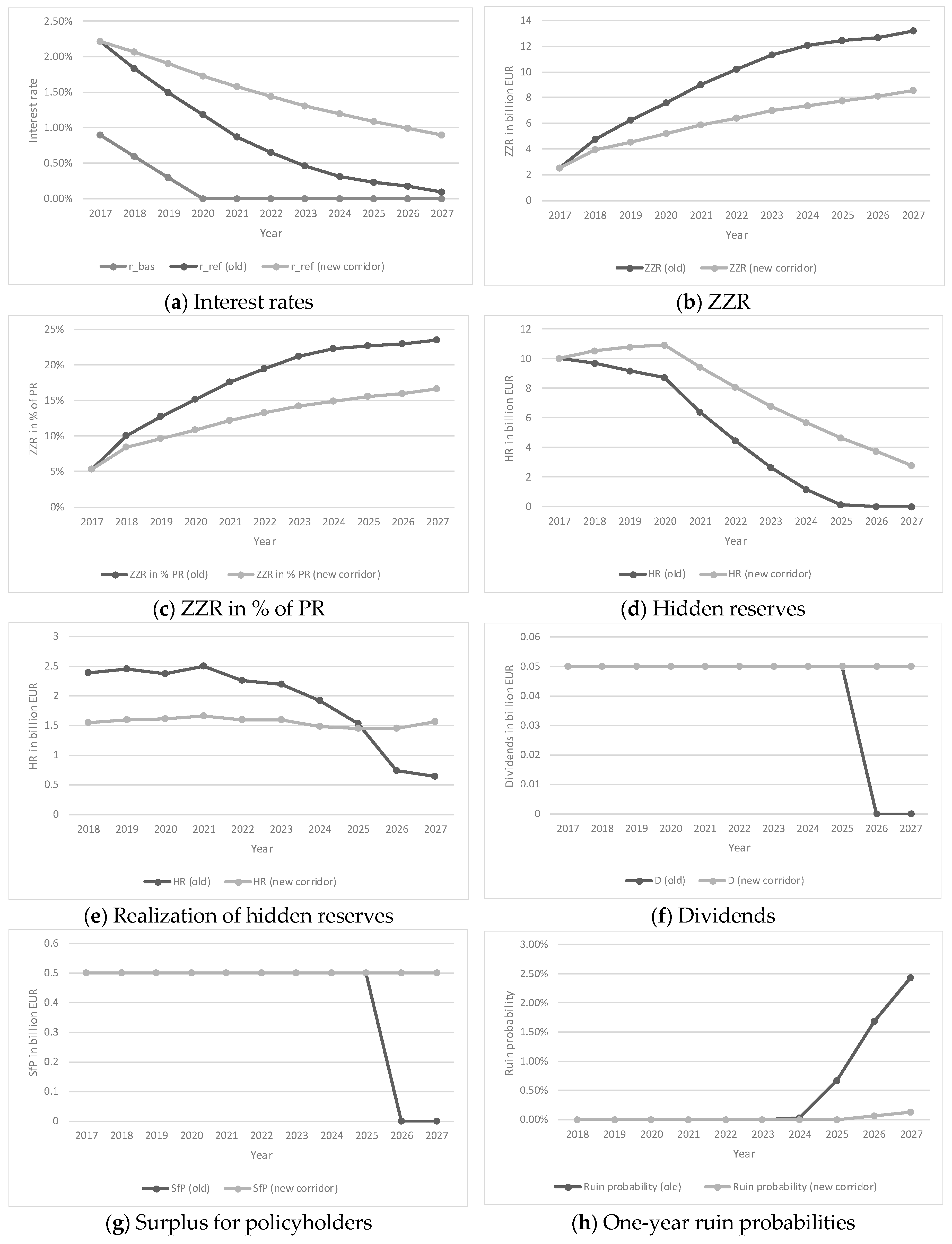
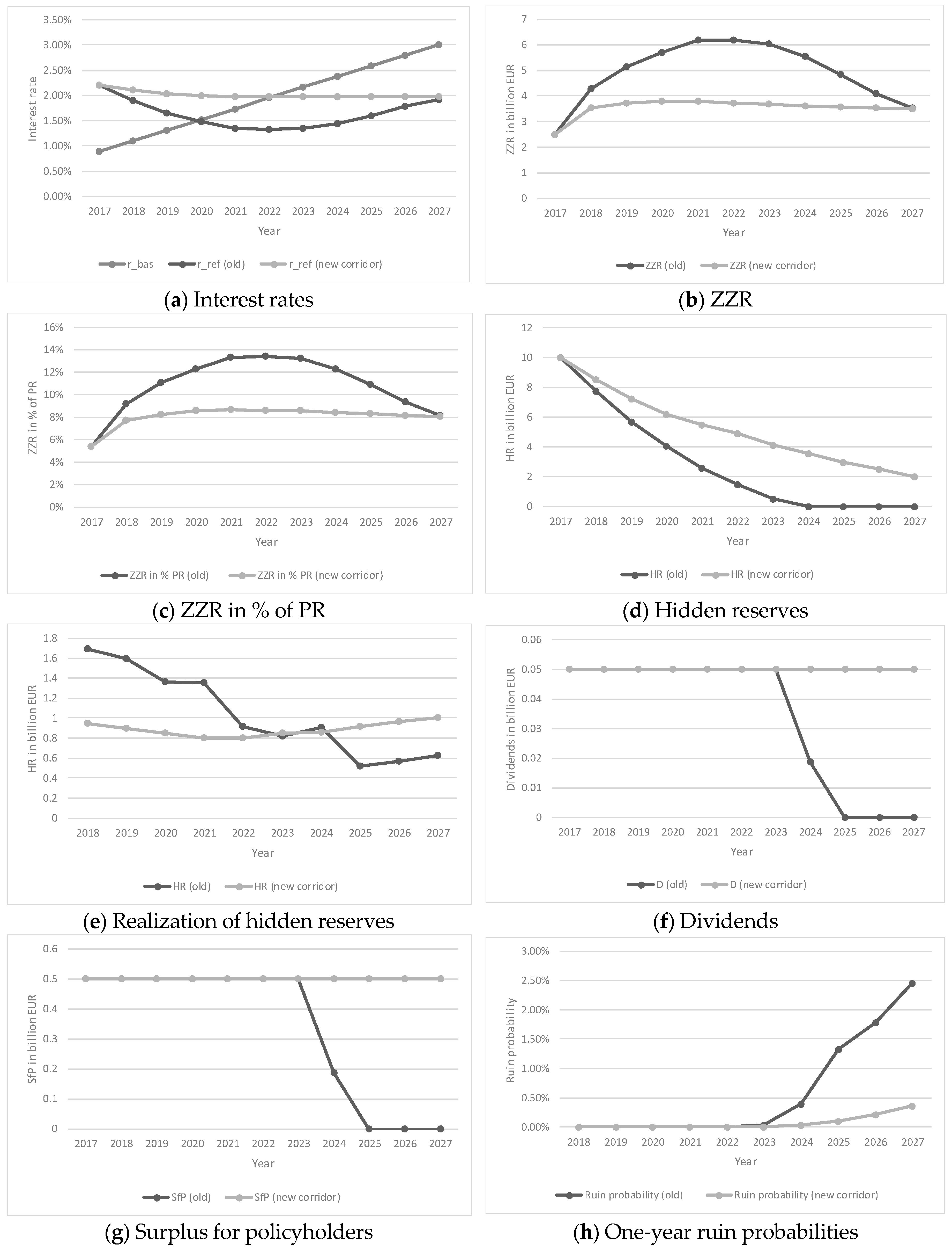
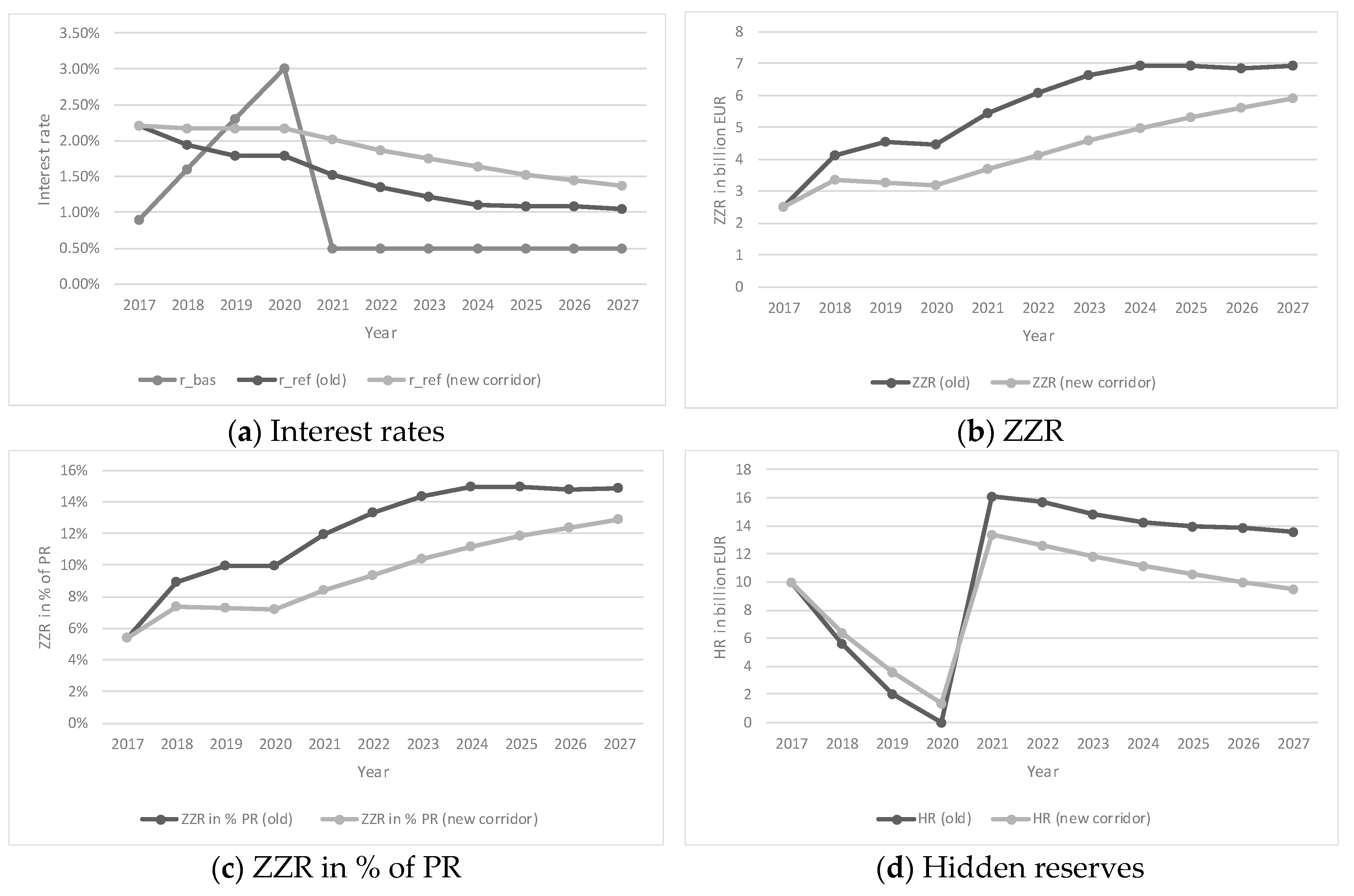
In the following subsection, the results of our Monte Carlo simulations (10,000 simulation paths) for each interest rate scenario are presented. Figure 1, Figure 2, Figure 3 and Figure 4 show the average future development of a life insurer under various interest rate scenarios, meaning that they display expected values.

3.2.1. Interest Rate Scenario 1

Our results in interest rate scenario 1 are given in Figure 1. In interest rate scenario 1, the basic interest rate was constantly 0.90% from 2017 to 2027 (see Table 5). Figure 1a shows that the reference interest rate $r_{ref,t}$, calculated using the old ZZR method, already reached the constant value of 0.90% in 2026 (since 2023 it was nearly 0.90%). In contrast, the reference interest rate ${\overline{r}}_{ref,t}$, calculated using the new corridor method, decreased much more slowly, and in 2027, was still 1.41%, since in the new corridor method the reference interest rate is only allowed to decrease within the corridor. As a result, the increase of the ZZR in billion EUR (Figure 1b) and in percentage of the total policy reserve (Figure 1c) was faster using the old method compared to the new corridor method. The ZZR using the old method reached its peak in 2024 and slightly decreased until 2027, while the ZZR using the new corridor method still increased until 2027, which is why the ZZRs in 2027 are closer together. For the years after 2027, it should be the case that they come even closer (with the ZZR slightly decreasing using the old method and slightly increasing using the new corridor method) until they are on the same level, since both methods aimed at the same amount. However, the old method reached that goal much faster than the new corridor method, which led to an even higher increase of the ZZR using the new corridor method.

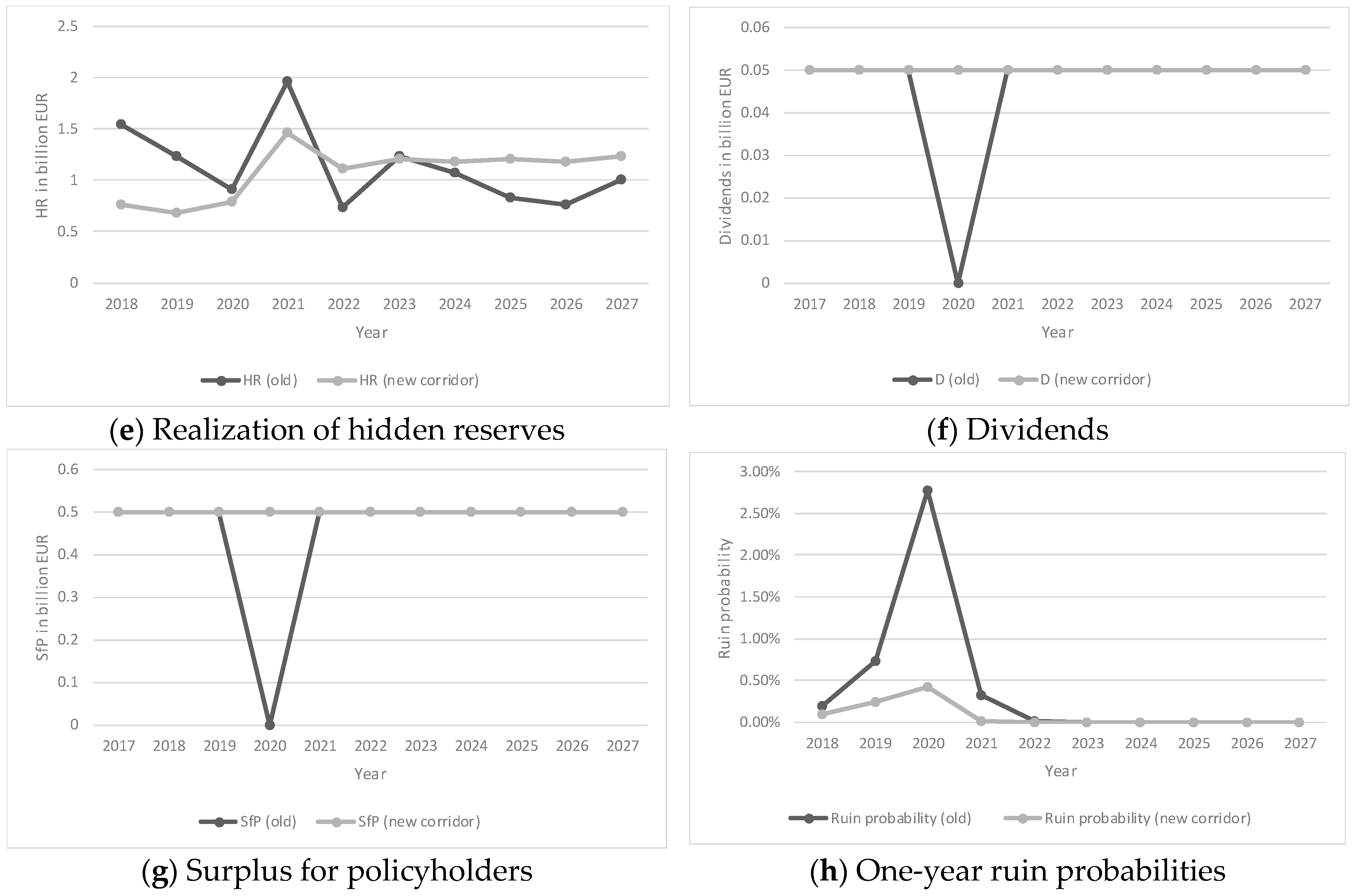
This can also be seen in Figure 1d,e, in which we see the hidden reserves over time and the respective realization of hidden reserves. Using the old method, the life insurer had to finance much more ZZR in the first years compared to using the new corridor method. Since, in this case, the gross surplus without the realizing hidden reserves was not enough, in the first years the realization of hidden reserves using the old method was much higher than using the new corridor method.4 Therefore, the hidden reserves decreased much faster using the old method than when using the new corridor method.

However, in both methods, dividends and surplus for policyholders could be kept constant over time (see Figure 1f,g). Therefore, in this scenario, in the first years the effort for the life insurer using the old method was higher than when using the new corridor method, where the efforts were more evenly distributed over time. However, in this setting, the effort was not too high for the life insurer, which can also be seen when considering the one-year ruin probability from 2018 to 2027, which is, in both cases, always nearly zero (see Figure 1h).5

3.2.2. Interest Rate Scenario 2

In interest rate scenario 2, the basic interest rate fell in the next three years evenly to 0.00% in 2020 and stayed at 0.00% until 2027. Figure 2 shows the corresponding results of our simulation analysis. While the reference interest rate using the new corridor method is only allowed to decrease within the corridor, again, it clearly decreased more slowly than when using the old method (see Figure 2a) and in 2027 was nearly zero (0.09%), as compared to 0.90% in the new corridor method. Similarly to interest rate scenario 1, Figure 2b,c show that the ZZR increased more quickly when using the old method than when using the new corridor method. However, in this scenario, neither method seemed to reach their peak until 2027 and the ZZR increased in both cases.

The hidden reserves of the life insurer (Figure 2d,e) rapidly decreased from 2020 onward using the old method, which is much faster than in the new corridor method; from 2025 onward they were nearly zero, while they were still 2.76 billion EUR in 2027 when using the new corridor method. Since the life insurer had more ZZR in 2027 using the old method, having more hidden reserves was not necessarily an advantage of the new corridor method in this case. However, Figure 2e shows that the realization of hidden reserves using the new corridor method was more even over time.

In particular, Figure 2f,g show the advantage of the more even realization of hidden reserves. Using the new corridor method kept more hidden reserves and allowed the life insurer to use the gross surplus over more years to finance the ZZR. As a result, the life insurer could keep their dividends (Figure 2f) and surplus for policyholders (Figure 2g) constant over time. In addition, the ruin probability in this case was nearly zero over the years (Figure 2h). However, using the old method, the life insurer had to finance very high increases of the ZZR, especially until 2024, which decreased their hidden reserves to zero. Since interest rates remained very low, the life insurer did not generate many new hidden reserves and did not have enough gross surplus to finance the remaining ZZR and dividends as well as the surplus for policyholders. Due to the critical situation of the life insurer, dividends and surplus for policyholders were zero in 2026 and 2027 (see Figure 2f,g). Moreover, the life insurer’s one-year ruin probability increased to 2.43% in 2027. Therefore, the results show that the fast increase of the ZZR using the old method was too much for the life insurer; in interest rate scenario 2, the new corridor method was more useful from the perspective of all the considered stakeholders (life insurer, regulators, policyholders and equity holders).

3.2.3. Interest Rate Scenario 3

In interest rate scenario 3, we assumed that the basic interest rate increased evenly over the next 10 years to 3.00% in 2027 (see Table 5). Figure 3a shows that using the old method, the reference interest rate decreased from 2.21% in 2017 to 1.33% in 2022, even though the basic interest rate increased from 0.90% to 1.95%. Using the new corridor method, the reference interest rate did not show such a lag effect, since it decreased only slightly and remained at 1.97% from 2021 onward. This was due to its definition in the new corridor method that did not allow the reference interest rate to decrease when in an increasing interest rate environment. In 2027, both reference interest rates were nearly the same (old method: 1.93%, new corridor method: 1.97%). Figure 3b,c then reveal a big disadvantage of the old method. Since the reference interest rate using the old method decreased until 2022, the ZZR increased and reaches its peak in 2022. In 2027, the ZZR was nearly the same in both cases, while the ZZR using the new corridor method was approximately at this level since 2018. As a result, using the old method, the life insurer first had to finance high increases in the ZZR, which was then no longer necessary and was reduced again. Using the new corridor method, the life insurer did not have to make this effort.6

Since the interest rates increased, hidden reserves decreased in both cases (see Figure 3d). However, using the old method, they decreased much faster and were zero from 2024 onward, while they were still 2.02 billion EUR in 2027 when using the new corridor method. Figure 3e shows the reason for this. Since the life insurer had to finance higher increases of the ZZR, they had to realize more hidden reserves. As a result, from 2024 onward, the life insurer was in a critical situation and did not have enough hidden reserves left to finance the aimed dividends and surplus for policyholders. In contrast, using the new corridor method, enough hidden reserves were left to keep constant dividends and surplus for policyholders (see Figure 3f,g).

Moreover, the one-year ruin probability increased to 2.46% in 2027 using the old method, as compared to 0.36% using the new corridor method.

3.2.4. Interest Rate Scenario 4

Finally, interest rate scenario 4 described a situation in which the basic interest rate first increases to 3.00% evenly over the next three years, before plummeting to 0.50% in 2021 and remaining there until 2027 (see Table 5). Figure 4a shows the corresponding reference interest rates. The reference interest rate calculated using the old method decreased every year to 1.04% in 2027, even when the basic interest rate increased. Due to its definition, the reference interest rate calculated with the new corridor method did not have such a lag effect. While the basic interest rate increased, it remains at 2.16% and decreased due to the corridor slower to 1.36% in 2027.

Accordingly, using the old method, the ZZR increased from 2018 to 2020 in a growing interest rate environment, while it decreased using the new corridor method. With the basic interest rate falling to 0.50% in 2021 and remaining there, both methods led to a rise of the ZZR, which resulted in a similar ZZR in 2027. However, the increase of the ZZR was more greater over the years using the new corridor method.

Interestingly, in this scenario, in 2027 hidden reserves were higher in the case of the old method in comparison to the new corridor method (see Figure 4d). The reason is that the life insurer, using the old method, had to finance a high ZZR, while the basic interest rates rose in the first years. As a result, the life insurer had to realize more hidden assets (see Figure 4e). However, in this interest rate environment, the life insurer can reinvest the money to relatively high-yield bonds, which provide the life insurer with higher market values and higher hidden reserves in the lower interest rate environment from 2023 onward. This might be an advantage of the old method.

However, financing a high ZZR from 2018 to 2022 in a high interest rate environment leads to critical situations for the life insurer. Figure 4f,g show that, in contrast to using the new corridor method, using the old method caused dividends and surplus for policyholders to be zero in 2020 due to a critical situation. Accordingly, in this time frame, the ruin probability when using the old method is much higher than when using the new corridor method. For instance, the one-year ruin probability in 2020 using the old method was 2.78%, as compared to 0.42% using the new corridor method.

4. Discussion

This paper compared two different methods for additional reserves due to low interest rates in the German life insurance industry: the old method and the new corridor method.

Modeling a typical German life insurer and using Monte Carlo simulation techniques, we holistically analyzed the effects of these different methods under various future interest rate scenarios from the perspective of various stakeholders (life insurer, regulators, equity holders and policyholders). Focusing on the effects of both methods on the reference interest rates or the liabilities of the life insurer, it is evident that the ZZR increased more slowly using the new corridor method as compared to the old method and that the new corridor method did not lead to lag effects as in the case of the old method. The introduction of the corridor in the definition of the reference interest rate in the new method led to a slower decrease of the reference interest rate and therefore a slower increase of the ZZR in Scenario 1 and 2, as well as in Scenario 4 in the years from 2021 to 2027. In our numerical study, the requirement that the sign of the change in the smoothed interest rate is the same as the sign of the change in the realized interest rate affected the periods of increasing interest rates, i.e., Scenario 3 and the years 2018–2020 in Scenario 4 by avoiding the time lag. However, only by comprehensively modeling a life insurer (including its assets and dependencies between assets and liabilities) as was done in this paper, can we fully analyze the effects of both methods. Only this allows to investigate whether the increase of the ZZR in the old method is too fast and whether the new corridor method provides a more suitable increase of the ZZR.

Our results show that using the old method leads to faster increases of the ZZR than using the new corridor method. This is not necessarily a bad thing; however, our analysis reveals that in three out of four interest rate scenarios, financing such a high ZZR led to critical situations for the life insurer. These critical situations resulted in an increase of the one-year ruin probability (that is higher than the aimed 0.50% Solvency II level), lower dividends for equity holders and a lower surplus for policyholders. In contrast, using the new corridor method, the ZZR increased more slowly but also more evenly and helped the life insurer to avoid such critical situations. Related to this, our analyses show that realizations of hidden reserves in low interest rate environments were typically higher using the old method. Reinvesting the money in such interest rate environments led to lower future asset returns, causing critical situations for the life insurer.

Moreover, our results confirm that using the old method led to lag effects, meaning that the ZZR increased even in an increasing interest rate environment. This was especially challenging because hidden reserves to finance the ZZR decreased in such an environment, which led to more critical situations for the life insurer. Since the new corridor method also avoided this problem and still provided a high level of ZZR when needed, the new corridor method seems to be a suitable solution to contend with the coming interest rate developments.

References

1. Albrecht, Peter. 2015a. Versagt die Bundesregierung beim Erklären der Zinszusatzreserve? Zeitschrift für Versicherungswesen: ZfV 66: 243–44. [Google Scholar]
2. Albrecht, P. 2015b. Zinszusatzreserve: Felix Austria? Zeitschrift für Versicherungswesen: ZfV 66: 346–48. [Google Scholar]
3. Albrecht, Peter, and Hermann Weinmann. 2015. Zur Diskussion um die Zinszusatzreserve in der Lebensversicherung: Legaler Betrug oder mangelndes Produktverständnis? Zeitschrift für Versicherungswesen: ZfV 66: 137–39. [Google Scholar]
4. Alexandrova, Maria, Alexander Bohnert, Nadine Gatzert, and Jochen Ruß. 2017. Equity-Linked Life Insurance Based on Traditional Products: The Case of Select Products. European Actuarial Journal 7: 379–404. [Google Scholar] [CrossRef]
5. Assekurata. 2016. Assekurata-Marktausblick zur Lebensversicherung 2016/2017. Cologne: Assekurata, Available online: https://www.assekurata.de/fileadmin/mediendatenbank/Dokumente/Publikationen/Marktausblick/2016/Leben/Assekurata_Marktausblick_Lebensversicherung_2016_2017.pdf (accessed on 9 September 2018).
6. Assekurata. 2017. Marktstudie zu Überschussbeteiligungen und Garantien 2017. Cologne: Assekurata, Available online: https://www.assekurata.de/fileadmin/mediendatenbank/Dokumente/Publikationen/Studieninfo/2017/Ueb/Praesentation_Studie_Ueberschussbeteiligungen_Garantien_2017_Homepage.pdf (accessed on 9 September 2018).
7. Assekurata. 2018. Assekurata-Marktausblick zur Lebensversicherung 2018. Cologne: Assekurata, Available online: https://www.assekurata.de/fileadmin/mediendatenbank/Dokumente/Presse/Pressemitteilungen/2018/Marktausblick_Leben/Assekurata_PM_17_07_2018_Marktausblick_Lebensversicherung.pdf (accessed on 9 September 2018).
8. Berdin, Elia, and Helmut Gründl. 2015. The Effects of a Low Interest Rate Environment on Life Insurers. The Geneva Papers on Risk and Insurance- Issues and Practice 40: 385–415. [Google Scholar] [CrossRef] [Green Version]
9. BMF. 2018. Referentenentwurf des Bundesministeriums der Finanzen—Dritte Verordnung zur Änderung von Verordnungen nach dem Versicherungsaufsichtsgesetz. Available online: https://www.bundesfinanzministerium.de/Content/DE/Gesetzestexte/Gesetze_Gesetzesvorhaben/Abteilungen/Abteilung_VII/19_Legislaturperiode/2018-Dritte-Verordnung-aenderung-von-Verordnungen-nach-Versicherungsaufsichtsgesetz/1-Referentenentwurf.pdf?__blob=publicationFile&v=2 (accessed on 19 September 2018).
10. Bohnert, Alexander, and Nadine Gatzert. 2014. Fair Valuation and Risk Assessment of Dynamic Hybrid Products in Life Insurance: A Portfolio Consideration. The Geneva Papers on Risk and Insurance Issues and Practice 39: 148–72. [Google Scholar] [CrossRef]
11. Bohnert, Alexander, Patricia Born, and Nadine Gatzert. 2013. Dynamic Hybrid Products in Life Insurance: Assessing the Policyholders’ Viewpoint. Insurance: Mathematics and Economics 59: 87–99. [Google Scholar] [CrossRef]
12. Bohnert, Alexander, Nadine Gatzert, and Peter Løchte Jørgensen. 2015. On the Management of Life Insurance Company Risk by Strategic Choice of Product Mix, Investment Strategy and Surplus Appropriation Schemes. Insurance: Mathematics and Economics 60: 83–97. [Google Scholar] [CrossRef]
13. Bohnert, Alexander, Johanna Eckert, and Nadine Gatzert. 2018. The Impact of Risk Classification in Life Insurance: An Analysis of Underwriting Risk, Underwriting Costs, and Classification Systems. Working Paper. Nuremberg: Friedrich-Alexander University Erlangen-Nürnberg (FAU). [Google Scholar]
14. Consiglio, Andrea, Flavio Cocco, and Stavros Zenios. 2001. The Value of Integrative Risk Management for Insurance Products with Guarantees. Journal of Risk Finance 2: 6–16. [Google Scholar] [CrossRef]
15. Dalmis, Özcan, Holger Hebben, and Matthias Matzke. 2013. Die Zinszusatzreserve im Aktiv-Passiv-Kontext. Zeitschrift für Versicherungswesen 64: 3–85. [Google Scholar]
16. DAV. 2016. ZZR—Zeit Zu Renovieren?! Cologne: DAV, Available online: http://www.qx-club.de/2016_03_01_ZZR_qx_Club_final.pdf (accessed on 9 September 2018).
17. DAV. 2017. Im Interesse der Kunden: Zinszusatzreserve muss neu kalibriert warden. Cologne: DAV, Available online: https://aktuar.de/fachartikelaktuaraktuell/AA39_Zinszusatzreserve.pdf (accessed on 9 September 2018).
18. Eckert, Johanna, Nadine Gatzert, and Michael Martin. 2016. Valuation and Risk Assessment of Participating Life Insurance in the Presence of Credit Risk. Insurance: Mathematics and Economics 71: 382–93. [Google Scholar] [CrossRef]
19. Eling, Martin, and Stefan Holder. 2013. The Value of Interest Rate Guarantees in Participating Life Insurance Contracts: Status Quo and Alternative Product Design. Insurance: Mathematics and Economics 53: 491–503. [Google Scholar] [CrossRef]
20. GDV. 2018. Die Deutsche Lebensversicherung in Zahlen 2018. Berlin: GDV, Available online: https://www.gdv.de/resource/blob/34084/953b4048365cf01fb254ba9175b0d948/lebensversicherung-in-zahlen-2018-data.pdf (accessed on 9 September 2018).
21. Hieber, Peter, Ralf Korn, and Matthias Scherer. 2015. Analyzing the Effect of Low Interest Rates on the Surplus Participation of Life Insurance Policies with Different Annual Interest Rate Guarantees. European Actuarial Journal 5: 11–28. [Google Scholar] [CrossRef]
22. Hieber, Peter, Jan Natolski, and Ralf Werner. 2019. Fair Valuation of Cliquet-style Return Guarantees in (Homogeneous and) Heterogeneous Life Insurance Portfolios. Scandinavian Actuarial Journal 2019: 478–507. [Google Scholar] [CrossRef]
23. Holsboer, Jan. 2000. The Impact of Low Interest Rates on Insurers. The Geneva Papers on Risk and Insurance Issues and Practice 25: 33–58. Available online: www.jstor.org/stable/41952510 (accessed on 16 July 2019).
24. Kling, Alexander, Andreas Richter, and Jochen Ruß. 2007a. The Interaction of Guarantees, Surplus Distribution, and Asset Allocation in With-Profit Life Insurance Policies. Insurance: Mathematics and Economics 40: 164–78. [Google Scholar] [CrossRef]
25. Kling, Alexander, Andreas Richter, and Jochen Ruß. 2007b. The Impact of Surplus Distribution on the Risk Exposure of With Profit Life Insurance Policies Including Interest Rate Guarantees. Journal of Risk and Insurance 74: 571–89. [Google Scholar] [CrossRef]
26. Reuß, Andreas, Jochen Ruß, and Jochen Wieland. 2016. Participating Life Insurance Products with Alternative Guarantees: Reconciling Policyholders’ and Insurers’ Interests. Risks 4: 11. [Google Scholar] [CrossRef]
27. Schmeiser, Hato, and Joël Wagner. 2014. A Proposal on How the Regulator Should Set Minimum Interest Rate Guarantees in Participating Life Insurance Contracts. Journal of Risk and Insurance 82: 659–86. [Google Scholar] [CrossRef]
28. Wieland, Jochen. 2017. Runoff or Redesign? Alternative Guarantees and New Business Strategies for Participating Life Insurance. European Actuarial Journal 7: 29–50. [Google Scholar] [CrossRef]
1
By “old high-yield securities”, we mean securities the life insurer has had in their books for a long time. Book value and market value for these securities differ particularly strongly from each other, implying high hidden assets.
2
We assume that the life insurer pays the annuities to the policyholders at the beginning of the year. Moreover, we assume that the life insurer pays the lump sum payments on maturity to endowment holders at the beginning of the year. However, lump sum payments on death are paid at the end of the year.
3
If P t + S t + S f P t + D t + > 0 , the life insurer must invest the money, which is why this increases the market value and the book value of assets exactly in that amount. However, if P t + S t + S f P t + D t + < 0 , the life insurer must pay the negative amount. The market value is therefore reduced exactly by that amount. However, the book value differs, possibly due to hidden reserves from the market value, and therefore must be reduced by an amount that has to be adjusted by the difference between the book and market values of assets. The philosophy behind this asymmetric treatment is the careful accounting principles of local GAAP in Germany.
4
Note that we neglected transaction costs. Taking transaction costs into account would have worsened the effect of realizing hidden reserves.
5
Note that the results using the new corridor method were based on x = 9 % (see BMF 2018). Sensitivity analyses for the new corridor method showed more similar results compared to the old setting using a higher x and less similar results using a lower x. This was also the case for the other interest rate scenarios.
6
Note that this also shows a problem regarding a fair distribution of hidden reserves among policyholders. Terminating policies obtain a share of hidden reserves. If hidden reserves are realized before terminating, this increases the surplus, in which policyholders also participate. However, since realized hidden reserves are used to finance the ZZR, policyholders do not participate in them. Only when the ZZR decreases does this allow the policyholders to participate. Therefore, in the case of the old method, the share of hidden reserves for policyholders with terminating policies, e.g., in 2022 was too low, while other policyholders (especially new policyholders) benefited, implying an unfair distribution among policyholders in the portfolio.
Figure 1. Simulation results in interest rate scenario 1.
Jrfm 12 00119 g001
Figure 2. Simulation results in interest rate scenario 2.
Jrfm 12 00119 g002
Figure 3. Simulation results in interest rate scenario 3.
Jrfm 12 00119 g003
Figure 4. Simulation results in interest rate scenario 4.
Jrfm 12 00119 g004aJrfm 12 00119 g004b