Abstract
The global financial market has become extremely interconnected as it demonstrates strong nonlinear contagion in times of crisis. As a result, it is necessary to measure financial systemic risk in a comprehensive and nonlinear approach. By establishing a large set of risk factors as the main bones of the financial market network and applying nonlinear factor analysis in the form of so-called PolyModel, this paper proposes two systemic risk indicators that can prognosticate the advent and trace the development of financial crises. Through financial network analysis, theoretical simulation, empirical data analysis and final validation, we argue that the indicators suggested in this paper are proved to be very effective in forecasting and tracing the financial crises from 1998 to 2017. The economic benefit of the indicator is evidenced by the enhancement of a protective put/covered call strategy on major stock markets.
1. Introduction
In the past two decades, the global financial market became highly interconnected. Any disturbance in the network-like system of the global economy can potentially trigger worldwide financial turmoil (Gray 2013). For instance, in the financial crisis from 2007 to 2009, the turmoil raged across many countries and various economic sectors, leading to serious financial systemic risk among global assets, and eventually resulting in the bailouts of major institutions by the US government, and likewise in other countries (see Acharya et al. 2012; Blancher et al. 2013).
Arguably, systemic risk is one of the main features of the contemporary global financial market. How to monitor and measure such a risk has attracted a significant amount of attention from the central bank, the market and the academia (Billio et al. 2012). Distinct from other financial risks that can be separated by assets or businesses, systemic risk cannot be easily defined. It manifests itself in various forms such as asset bubbles, liquidity crises, market panic, abnormal events, regional political unrests, series of failures, etc. All of the above issues might escalate from a regional problem into a global one and eventually cause turmoil in the global financial system by contagion (see Brunnermeier and Cheridito 2014; Brunnermeier and Sannikov 2012).
In fact, contagion is the most salient feature of systemic risk and it has characterized each financial crisis on the global scale in history. Hü (2015) made a detailed survey on the literature of interbank network in his article about too interconnected to fail and introduced the effect of network structure on contagion. In their article, Glasserman and Young (2016) pointed out that although network connections diversify risk exposure, they also create channels through which shocks can spread by contagion. Acemoglu et al. (2015) argued that the complex interconnection of financial system can help diversify the risks of small shocks, but will amplify the risks stemming from large shocks by contagion. Generalizing the ideas from literature, we summarize three levels of contagion. The first level is the most direct one. For example, let us assume that company D owns assets of company C, who owns assets of company B and that company B owns assets of company A. If A defaults, B will face liquidity problem and default C who in turn, will default D. The literature on contagion in financial networks often stays at this level. However two other levels, much more devastating, occur upon a systemic crisis. The second level materializes when the first level gradually deteriorates the borrowing conditions, as well as companies’ market values, making borrowing costs become prohibitive (Sorkin and Hughes 2009). The third level is the most serious. It occurs when the global panic spreads over international markets. Trust is destroyed, and nobody is willing to lend. Flight to quality results in assets becoming illiquid, while their value plummets rapidly, finally leading to a financial crisis (see Sornette and Anderson 2002; Sornette et al. 1996; Sornette and Johansen 1997, 2001; Sornette and Zhou 2006).
Therefore, the definition of systemic risk should be related to a network event, whereby the failure of one institution propagates to other institutions by “domino effect”, loss of borrowing capacity and flight to quality. The consequence of such an event is often catastrophic because it implies a loss of trust and a liquidity crisis. The joint drop of asset prices and risk factors reveals the high correlation, conditionally to large moves, a typical feature of nonlinear PolyModels. We observe that the whole market is almost fully explained by the dominant risk factors especially when the crisis is coming. Therefore, without losing common sense, we here define systemic risk by its observable effects, rather than by the description of a macroeconomic mechanism, be it spread over the entire financial system, because such mechanisms only partially reflect the true market forces at stake. Our systemic risk indicator is defined as the average explained risk of the market by each risk factor.
The rest of paper is organized as follows: Section 2 is a literature review on the topic. Section 3 describes the mechanism of a systemic event by network analysis, risk decomposition and aggregation. We show the stochastic simulation of risk and the derivation of systemic risk indicator. Section 4 demonstrates the nonlinearity feature during a financial crisis and introduces the nonlinear PolyModel theory. Section 5 proposes our PolyModel-based systemic risk indicators with historical weekly data and shows their efficacy as early warning of financial crises. Section 6 introduces investment strategies on the S&P500 Index and its options, based on the indicators, as a validation of our results. Section 7 concludes the paper.
2. Literature Review
Patro et al. (2013) proposed systemic risk indicator by analyzing correlations among the equity of financial institutions. However, they calculated with the normal distribution and took no consideration for the skewness and kurtosis, the fat tailed problems. Balla et al. (2014) applied Extreme Value Theory to derive extremal tail dependency among stock returns of large U.S. depository institutions as an indicator of systemic risk. Although extremal tail dependency accounts for fat tailed distribution, it still cannot measure the systemic risk in a holistic scenario and ignores other hidden signals that might not be very obvious or intuitively reasonable at first glance but could impact financial institutions which would then strike the whole market. Other risk measures, such as Marginal Expected Shortfall (“MES”, Acharya et al. 2010), Distressed Insurance Premium (“DIP”, Huang et al. 2009) and Conditional Value at Risk (“CoVaR”, Adrian and Brunnermeier 2014) share the corresponding limitations mentioned before. From our perspective, the whole financial system is a network with lots of possible turbulences and is unstable in itself, any unpredictable shocks can lead to systemic turmoil. Therefore, we should not measure systemic risk only within a certain or several financial asset classes but from a global network perspective (see Rama et al. 2009; Hansen 2013).
Defining the financial system as an interbank network and analyzing the mutual asset and liability among them, Acemoglu et al. (2015) found that the factors contributing to great systemic risk in the market under extreme downturns are also the ones that enhance stability because of the diversification. In addition, their analysis shows that the business interactions exhibit nonlinearity feature in the network. Brownlees and Frison (2014) researched into the cross-sectional correlations of a large set of risk factors by establishing a factor-network. Their research reveals the high interconnectedness and centrality of macro, credit and interest rate risk factors. Similarly, they also mentioned that the factor-network methodology is robust to nonlinear dependence across the factors. Both studies mentioned above provide us a new viewpoint to understand systemic risk in a nonlinear perspective of network.
Hartmann et al. (2015) proposed a novel systemic risk indicator by employing Markov-Switching Vector Autoregression model, which can dynamically capture the nonlinear relationships between macroeconomic variables. They pointed out that the market has different regimes under different economic conditions. After shock testing, they found that the differences between Impulse Response Functions (IRF) from normal market and crisis regimes are striking and suggested that risk models should allow for nonlinearity because regime switching heavily impacts coefficients in linear model. These results further prove that financial market behaves like a regime switching model with nonlinear effect.
The subprime mortgage crisis attracts a growing research on financial networks and complicated network models has been developed to analyze the problems of interbank system (Chen 2010). Langfield and Soramäki (2014) put forward that multilayer financial networks can capture the different types of business transactions such as lending, repurchase agreements or derivatives among banks. In addition, interbank network exhibits a core-periphery structure. Fabio Caccioli et al. (2015) revealed that the systemic risk can propagate by direct and indirect links in the entire financial system.
In this study, we propose a class of our systemic risk indicators based on the decomposition and aggregation of a simplified network structure with nonlinear dependence. We construct a large set of risk factors as the main skeleton of the financial network and decompose the risk of the financial system explained by each risk factor into three independent components: systemic risk, factor specific risk and residual risk. To capture the nonlinear regime switching in the market, we follow the PolyModel logic and apply multiple single-factor regressions and aggregate all of the decomposed parts to acquire our systemic risk indicators which are finally measured as the contagion among these market representative risk factors. In summary, there are three main innovations in our paper: the first one is describing financial systemic risk with a large set of risk factors which we see as the main structure of financial network. The second one is decomposing the whole market risk into three components and then aggregating them. The third one is proposing systemic risk indicators with nonlinear factor analysis by PolyModel.
3. Network Analysis of Systemic Risk
Systemic risk, just as its definition in our study, is the risk that is systemically existing in a complicatedly interconnected network system (see Moore and Zhou 2012). By measuring such risk, we can provide insight of the structure of the global financial network which is deeply influenced by various related risk factors (Armentia et al. 2015).
In this paper, we argue that market representative risk factors should be analyzed as fundamental references to evaluate values of financial assets in business activities. Macro economic data such as GDP, CPI, PPI and balance sheet data could be the important risk factors but we do not include them into our risk factors set, because, on the one hand, these economic data lags behind the financial market, on the other hand, they will only be reported quarterly but we use historical weekly data to propose our systemic risk indicator. Thus, we only select market risk factors, which can cover the markets of main countries as well as different asset classes and are the basic benchmarks for the global financial market. Conforming with such selection criteria, we choose stock indexes, currency exchange, bond yields, interest rates, commodities, specific sectors and industries, volatility indexes, etc. as the market representative risk factors. Stock indexes from developed, emerging and frontier markets are very obvious to be the factors because they are very correlated in current stock market. A disturbance from any market will spread into other ones. Currency exchanges from different regions are also very important due to such an interconnected global capital market. A big appreciation or depreciation of them implies the regional financial issue which could further affect other regions. Bond yields represents the credit and debit cost in financial market and are the good indicators of the capital trust which can result in capital freeze and then liquidity crisis. Interest rates are the baselines for the pricing of all different assets and capital activities because their mutual interaction with currency exchange can cause big contagion shock in global market. Commodity prices reflect the raw materials cost for those companies involved in entity economy and include rich information about some systemic economic indicators. Specific sectors and industries should also be taken into consideration because as we all know that a big crisis is always indirectly triggered by one or two of their collapses. Volatility indexes measure the investors’ sentiment, indicate the market fluctuation and are nice indicators of fear which is fatal to financial market. In general, we try to collect as many risk factors as possible, even some of them are insignificant. That is because we aggregate all the risks explained by them without disregarding any one of them to make a horizontal comparison from 1998 to 2017.
Those factors are the risk sources of the assets, which means that any impact to the market is always caused by the disturbance in those risk factors first. So to measure systemic risk, we should establish the financial network including all of them. Thus, we construct the financial network as the interconnectedness of whole market representative risk factors which are supposed to contain all the market information. Details in choosing the market representative risk factors will be introduced in the section of empirical data analysis (Markovic and Urošević 2011).
Figure 1 shows the structure of financial network that is composed by a large set of risk factors and is the framework for us to perform theoretical systemic risk analysis in the following sections.
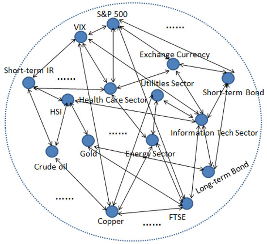
Figure 1.
The Structure of Financial Network.
3.1. Decomposition and Aggregation of Financial Risk
The interconnectedness in Figure 1 is so sophisticated that it is very difficult for us to quantify the connections among financial network. Instead of directly researching into the complex interconnectedness, we focus on how much on average the market representative risk factors explain the systemic risk.
3.1.1. Financial Risk Decomposition
Systemic risk is a contagion collapse of the whole financial market, a phenomenon like an inner explosion that spreads out and finally contaminates the entire financial network. In this paper, we decompose the risk of whole financial system into two independent components, systemic risk and factor specific risk . The formula-based explanation of the decomposition is detailed in next section with that of aggregation.
In Figure 2, systemic risk is the red solid circle with the radius indicating its degree, whole financial network is the big blue circle, risk factors are the small nodes. The nodes outside the red solid circle mean that these risk factors can fully explain the systemic risk but still have their own positive specific risks . The nodes inside the red solid circle mean that these risk factor cannot fully explain systemic risk but still have their own negative specific risks . For example, the risk explained by factor VIX index is the sum of and while that by factor energy sector is the sum of and , where but . In reality, the growth in the weighted average of risks explained by factors indicates the increase of the contagion in financial system where all the inner risk factors becomes strongly correlated. So systemic risk here is measured as the weighted average of risks of financial market explained by the risk factors.
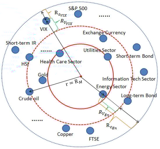
Figure 2.
The Change of Financial Network.
In Figure 2, we can also observe that as some blue nodes, the risk factors, move towards outside, the red solid circle, systemic risk, grows bigger into red dotted one. The most significant risk factor will have the biggest positive specific risk and the most insignificant risk factor will have biggest negative specific risk at the same time point. In addition, the specific risks will shrink to zero if the systemic risk dominates the whole financial risk under the worst market.
3.1.2. Systemic Risk Aggregation
From the above decomposition analysis, we already have two independent risk components of systemic risk and factor specific risk. In this section, we deduce both of these two components as well as the third one, residual risk, from the three sums of squares formula using nonlinear regression rather than linear. The underlying reason we apply nonlinear fitting will be discussed in more detail in Section 3.
Assuming we now have a large log-return dataset of n risk factors and log-return dataset of financial market index Y, we denote n nonlinear single factor regressions of Y over as and the corresponding explained sum of squares and unexplained sum of squares as and , which are orthogonal components. Samples of Y are marked , each has a predicted value . is the mean of Y and the residuals of prediction model are .
The equation of three sums of squares:
Suppose now we have n nonlinear single factor regressions with the same sample data Y and each of them has the same formula as above:
Here suppose:
As we mentioned before, the systemic risk is measured as the weighted average of explained risks, so we add the weights based on the values of all the and multiple corresponding equation with them as:
where and sum them up:
Now, let:
Next, let , which are actually the factor specific risk parts and it is obvious that changes from positive to negative as i goes from 1 to n. The negative ones mean that these risk factors cannot fully explain the systemic risk so we do not take them into consideration in the following deduction. Replace each which has non-negative in the above sums of squares equations with as follows:
and again multiple these equations with the weights based on the values of :
where . Summing them up again, we have:
Now, the variance estimation of Y is:
and let:
we then have:
and aggregate the group of equations above into:
where , the risk of Y, is decomposed into three parts: the systemic risk that is measured as the weighted average of the explained variances of financial market by all the risk factors, specific risk that is the weighted average of non-negative factor specific risks and residual risk that is the weighted average of regression residuals. This systemic risk aggregation demonstrates the overall risk explanation level by all of the market representative risk factors and is a good indicator accounting for nonlinearity and in the perspective of network structure.
3.2. Stochastic Process of Financial Market
In the last subsection, we decomposed the market risk explained by each of the risk factors into three components: systemic risk, factor specific risk and residual risk. Assume that the systemic risk component captures all the contagion effect in the financial market, those specific risks are the risks only explained by the specific risk factor and residual risks are just the noises, so the three components are totally independent. Now we suppose that the financial market price is a stochastic process over each risk factor defined as:
Because of the heavy tail phenomenon in the financial market, we arbitrarily choose and as levy processes with student’s T increments, , , while is a Brownian motion, . Then, we have:
where .
To demonstrate the stochastic process assumption is reasonable, it is necessary for us to simulate it by choosing one certain set of parameters for the distributions. Here, we set , = 3, and simulate 10 market evolution paths over 10 risk factors just to show the different influences from those components in the stochastic process. Figure 3 indicates that the risk of the whole financial market is composed by three components. We can see that the tails of systemic risk component globally impacts the whole market while those of specific risk component only locally affects the whole market and that the residual risk is the common stochastic noise in the market. In this figure, the 10 paths are the stochastic processes of financial market explained by each of the 10 risk factors and the total financial market stochastic process explained by all the risk factors can be seen as the weighted average aggregation of them. In this sense, the financial market risk is similarly considered as three parts: systemic risk, factor specific risk and residual risk.
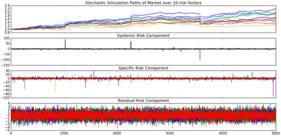
Figure 3.
Stochastic Process Simulation of Market.
3.3. Systemic Risk Indicators
Since systemic risk is the contagion part in financial market, the main objective in monitoring financial crisis is to measure this component. Systemic risk is the weighted average of nonlinearly explained risks of the financial sector by the whole risk factors. However, to simplify the indicators as the common statistical parameters, we first propose two systemic risk indicators and as follows. The general definition of is:
Combined with Equation (1), we get the first systemic risk indicator is:
In addition, we propose the ratio of systemic risk to specific risk as the second indicator:
where . We can see that the first systemic indicator is the weighted average of ’s and proportional to the ratio of systemic risk to the variance of financial market log-return Y, indicating what percentage the systemic risk can explain the total risk of financial market and that the second systemic risk indicator is the ratio of systemic risk to specific risk , signaling the dominating degree of over when crisis is coming.
Interestingly, after the empirical data analysis, we discover that these two indicators can give us an alternative view that their deep downturns are better than highly spikes in predicting financial crisis. So we define another two indicators and by inverting and as:
to give intuitive sense and facilitate final validation in Section 5.
4. Nonlinear PolyModel
Linear risk models are the most popular risk measures in the academic and financial industries because linear analysis can simplify many complicated problems and provide us with a clear result (Coste et al. 2011). However, few people have provided insights about whether the linearity is applicable in some other extreme situations. professionals and scholars usually assume linearity in their work since they see it as appropriate in analyzing normal business period. As a result, they adopt a linear analytical approach even in time of financial crisis (Dhillon et al. 2013). However, we argue that the sole use of linear approach is not adequate in understanding the crisis. From historical data, using only linear risk models have been proved a failure in predicting financial crises. As we propose in this study, a nonlinear approach should be used in measuring tail risk.
4.1. Nonlinearity Simulation
Stoyanov (2016) pointed out the pitfalls of linear risk models through the property of temporal aggregation that low frequency returns can be aggregated by higher frequency returns. For example, weekly return can be the sum of 5 daily log-returns. In his study, he shows that the linearity holds true for lower frequency returns if the high frequency returns exhibit linear dependence but that the linearity convergence from high to low frequency returns is getting slower when the high frequency returns have deterministic dependence with heavier-tail distribution. In addition, the slower convergence just indicates that the nonlinearity feature under this temporal aggregation property is true in the financial market as well. With the purpose to demonstrate the nonlinearity, we simulate his result as follows (see Stoyanov et al. 2010; Stoyanov et al. 2011).
Figure 4 displays that the deterministic dependence of simulated intra-day data where variable X is normally distributed converges to linear dependence as the frequency decreases to daily, weekly and monthly. Figure 5 shows that if the intra-day data where variable X obeys heavy-tailed T-distribution (degree of freedom = 2), the deterministic dependence slowly converges to linear dependence as the frequency decreases so the nonlinearity feature is very obvious within weekly and monthly data.
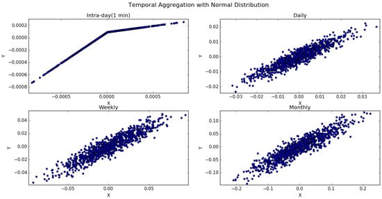
Figure 4.
Temporal Aggregation with Normal Distribution.
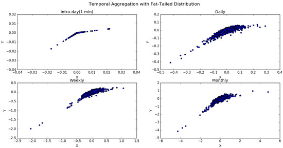
Figure 5.
Temporal Aggregation with Fat-tailed Distribution.
Therefore, the temporal aggregation simulation reveals the pitfalls of linear risk model when the assumption of homogeneous data violates and the data belongs to fat-tailed distribution.
4.2. Nonlinearity in Financial Market
With the fear of financial crisis spreading all around the world, nonlinearity feature appears as the consequence of liquidity crisis. However, such transition cannot be captured by linear models could not be captured by pure linear models and that even fat-tailed models could not well explain the unusual behavior during crisis, a dangerous cyclical cascade of market events as Figure 6.
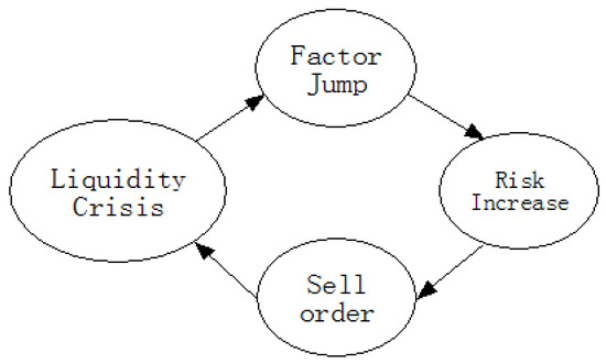
Figure 6.
Cyclical Cascade of Market Events.
Figure 7 shows the linear and nonlinear regressions of S&P 500 Index over two risk factors we choose. Here, the MXJP0FN Index is the Japan financial sector of MSCI and MXEF0FN Index is the emerging market financial sector of MSCI. In addition, samples are the historical weekly data of them during 2007–2010 when the great crisis happened. In Figure 7, we can see that the nonlinearity is very obvious in the left down side points which represent the nonlinear drops during crisis. Therefore, instead of linear risk models, we should apply nonlinear risk ones to capture the tail risk and explore the systemic risk.
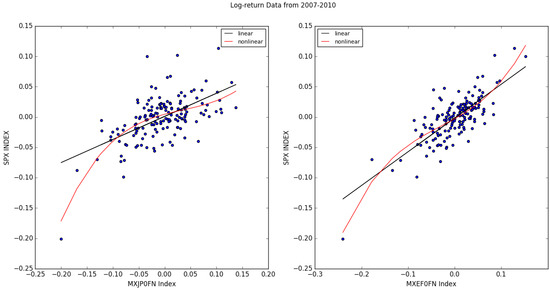
Figure 7.
Linear and Nonlinear Regression.
4.3. PolyModel Theory
Cherny et al. (2010) used nonlinear PolyModel to measure extreme risk of fund of funds. PolyModel, just as its name implies, is a collection of multiple models (Raphael and Zovko 2014). Denote Y an asset return variable and market risk factors. The first step is to regress Y on each with nonlinear functions:
where can be a linear combination of any nonlinear basis functions :
The second step is to merge all the equations above:
Then:
In practical, assuming the joint probability distribution of risk factors is Gaussian copula, we apply Hermite polynomials as the basis functions:
and solve out the coefficients through multiple-dimensional linear systems.
4.4. PolyModel Application in Systemic Risk
PolyModel uses nonlinear regression to capture the contagion risk in the market and is a good measure for extreme systemic risk when financial crisis is coming. However, in linear factor analysis model and time series model, we can only add several significant risk factors into model because the more risk factors we add, the more information we can collect, but the more uncertainty we will have. Hence, the common method is to evaluate the factor analysis and time series models with AIC or BIC. Likewise, in PolyModel, only the most significant ones will be selected based on information ratio but discard all the others.
In our risk decomposition methodology, the risk contribution to dependent variable Y from each risk factor includes systemic risk part that dominates the whole risk during financial crisis while is not significant when the market is normal. It cannot help us find out how much the general systemic risk within them if only measuring the risk contributions from several risk factors, so in fact we miss the hidden information contained in all the other factors. Figure 8 illustrates the hidden systemic risk missed in some risk measures that based on scanning for significant risk factors. In this figure, the red nodes lying outside the red dashed circle represent the most significant risk factors, the orange ones depict the less significant ones and the blue ones indicate insignificant factors. However, it is very possible that the large number of the disregarded orange nodes are very close to the most significant threshold. It is reasonable in first glance that we scan out the important ones but is problematic if we think it over, because we miss the global systemic risk hidden inside the red dashed circle, so we should evaluate the risk with the information from as many factors as possible.
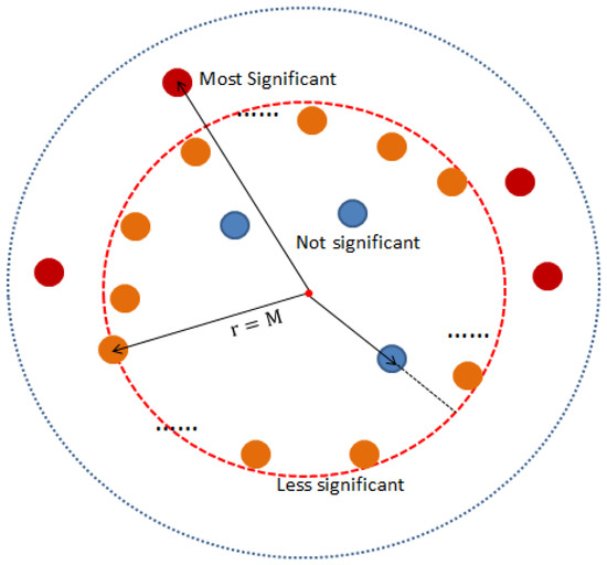
Figure 8.
Illustration of Hidden Systemic Risk.
Luckily, PolyModel has already provided us with a powerful tool to measure systemic risk in nonlinear methodology and the thought to merge risks. In this study, we adopt nonlinear regression methodology from PolyModel but modify its risk aggregating idea into weighted average risk, which we consider as systemic risk component. The next section will demonstrate the practical application with nonlinear PolyModel in measuring systemic risk and showing our systemic risk indicators with empirical data.
5. Empirical Data Analysis
In this section, we implement our idea discussed above with empirical data to propose our systemic risk indicators. We choose a large set of market representative risk factors from different asset classes and extract indicators from their historical data with nonlinear PolyModel fitting. Then, we analyze the effects of our systemic risk indicators by comparing with the large financial crises happened from 1998 to 2017.
5.1. Data Selection
In data selection, the most important part is the selection the market representative risk factors, which can well describe the landscape of the whole financial system. The financial market is mainly composed of stock, interest rate, bond, commodity, FX, derivative, etc. For stock, the stock indexes of different countries and different sectors are good enough to be the risk factors because they are almost the benchmark for the global stock market. For interest rate, the overnight rate, three month rate and different terms rate should be the necessary risk factors for many bank business activities. For bond, we should concern with the short, medium and long term government bond and corporate bond yields, which are the key factors of bond market. For commodity, their prices are very important risk factors for many economic activities which eventually will affect the financial transactions. For FX, of course, the exchange currency rate of different countries is another vital risk factor that can displays this country’s overall economy situation. Derivative is the financial products based on the actual underlying assets mentioned above, we should also collect some special information from them.
Finally, we choose nearly 200 risk factors within the groups mentioned above as the market representative financial networks and the S&P 500 Index as the dependent variable in our PolyModel fitting.
In measuring systemic risk, the periodic choice of log-return data can greatly affect the result. Daily data is the popular choice for research on risk, but it is very obvious that we cannot perfectly match all the daily data of these nearly 200 risk factors. Many funds prefer monthly data to construct their risk parity portfolios, especially mutual funds because the transaction fee is a considerable cost for them. However, we think that it is very possible that some big falls will happen just within one month and will be missed by using monthly data. Balancing the difficulty and defect above, we finally choose weekly historical data to explore the systemic risk indicators. In addition, the moving window size is a critical element in capturing the signals because long window size weights out some significant information within it while short window size means we use small amount of weekly data points, which makes the regression unreliable. After many tests with different window sizes, we decide to shift the data window by 26 weekly points.
5.2. Nonlinear PolyModel Fitting
We have already introduced nonlinear PolyModel and its application in analyzing the systemic risk within financial network in Section 3, so now we demonstrate how it works in extracting systemic risk indicators in real market data.
Coming to nonlinear PolyModel fitting, it is very important to choose adequate nonlinear polynomials basis. The most common basis is:
Supposing the probability distribution of dependent variable Y is the Gaussian copula of the risk factors, the PolyModel theory applies Hermite polynomials as the fitting basis because the variable distribution of the basis should be Gaussian family. In fact, practical applications show that the orthogonal basis is better in fitted results than the common basis. The probabilist’ Hermite polynomials are given by:
and the first 5 probabilist’ Hermite polynomials are:
After practical test, we find that the polynomial degree 4 is enough in nonlinear fitting so only the first 5 Hermite polynomials are included. Then, choosing the log-return of S&P 500 Index as Y, we regress it against each of our risk factors with nonlinear Hermite polynomials basis.
In normal business time, the volatility in financial market is small and the linear model runs well in measuring risk. However, when the big downturns or financial crises come, the volatility grows up and the nonlinear feature appears. We choose two nonlinear single factor regression models to demonstrate this phenomenon. Figure 9 shows the comparison of linear and nonlinear fitting with the data during normal and crisis period, which is regressed with half a year weekly data sets respectively. In this figure, MXJP0FN Index is the MSCI Japan financial sector and MXCN0FN Index is the MSCI Chinese financial sector. The green square points are the data during normal time and you can observe that the linear and nonlinear fitting are almost the same, making no big difference, because all of the data points concentrate in the middle. While the blue round points are the data during crisis time and you can find that the nonlinear fitting is better at capturing the extreme points than linear one because the data points disperse away from the middle. These two plots perfectly demonstrate that nonlinear PolyModel is very suitable to measure extreme systemic risk.
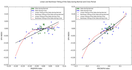
Figure 9.
Linear and Nonlinear Fitting.
5.3. Systemic Risk Indicators Analysis
In Section 3, we proposed two systemic risk indicators through Equations (3) and (4). Now after nonlinear PolyModel fitting, we have value for each one single factor model of financial sector Y against corresponding risk factor. Then, the indicator is the weighted average of all the 200 models and is the ratio of over the weighted sum of the differences of the ’s greater than and . From 1998 to 2017, we calculate both and at every week time point through nonlinear PolyModel fitting based on the weekly log-return data within a moving window size of half a year.
Figure 10 shows that our indicators and trace the financial crises very well. and basically have the same trend but seems a little bit volatile but more significant especially at crisis points. Referring to the vertical navy blue lines that represent the time crisis events occurred, we can observe that indicator and increase to a high level during Russian crisis. Again we can see that the indicators elevate during Dot-com bubble crisis and spike into a very high level after 911 Attack aggravated the crisis, which lasts further into 2003. The low level of indicators during 2003–2006 displays the steady growing market but the immediate increase in the later 2006 and early 2007 is an obvious warning signal for Sub-prime crisis. As one review on 2007–2008 Financial Crisis by Manoj Singh said that from February to March 2007, more than 25 Sub-prime lenders filed for bankruptcy followed by the well-known case of New Century Financial in April. The indicators stay at a high level from February to July 2007, well signaling the Sub-prime crisis beginning in July 2007 and eventually spike into a historical high level in August 2008 when Lehman Brothers filed for bankruptcy. Later, the same phenomenon that the increase in indicators happens again during the European Sovereign Crisis in later April 2010, US Sovereign Credit Degradation in early August 2011 and Chinese stock market turbulence in later August 2015.
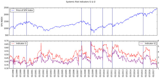
Figure 10.
Systemic Risk Indicators and .
Table 1 lists the reaction results of indicators and and shows that they trace well the evolution of all the previous financial crises.

Table 1.
Financial Drops vs. Reactive Indicators.
Although indicators and trace well all of these crises, basically are limited in predicting them with a certain time period in advance. For example, the spikes of the indicators in August 2008 and April 2010 are very abrupt and come together with the big drops. This limitation is actually the common feature for the systemic risk indicators in current literature. Therefore, finding the appropriate indicator to shed light on the early warnings of financial crisis is very important.
Taking a careful look at the indicators and , you can observe that there are deep downs in them just before the spikes together with the big drops at the crises. We can predict financial crises with some early warning time if these signals are useful as we expect. To make good use of these deep downing signals, we inverse to get by:
and inverse to get by:
So now let us reverse our logic of up and down in and to down and up in and . Figure 11 shows that just before every crisis, there is a significant increase in indicators and . Prior to Russian Crisis in August 1998, indicators and spike very high just before the big drop. The same as in Dot-bubble Crisis beginning in March 2000, they reach a very high level before the gradual downturns afterwards. In addition, we also can see that the spike occurs again just prior to the final big drop of Dot-bubble Crisis around April 2002. The sudden increase in February 2007 provides us with early warning signal of the subsequent great Sub-prime crisis in 2007–2008 and they again increase into a high level just before the serious downturn in August 2008. Likewise, just before European Sovereign Crisis in later April 2010, US Sovereign Credit Degradation in early August 2011 and Chinese stock market turbulence in later August 2015, indicators and go up into high level. All of the analysis above tells us that indicators and can provide us with earlier warning time than and in predicting financial crises. Besides, we will also show you in next section that this phenomenon even appears in some small drops as well.
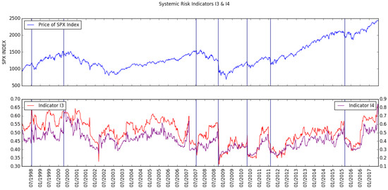
Figure 11.
Systemic Risk Indicators and .
The deep downturn in indicators and actually refers to the small weighted average and the low contagion level in the market. In practical terms, the different asset classes and regional markets will be balanced when the whole global financial system fluctuates normally, so the contagion level keeps normal fluctuation as well. However, some sectors, asset classes or regional markets, will turn into a bubble and the other counterparts lag behind them, which will decrease the market contagion level. There are two ways to get the contagion level back to normal, the lagging ones grow following the bubble or the bubble collapses to bring down the lagging ones together. For the latter way, if the big bubble immediately breaks, the whole financial system will become very correlated and the contagion level will increase back and even to be a higher level than normal because of the panic spreading around the financial world. Contrarily, the former way means the unsustainable bubble will temporarily further spread into the whole system, but will eventually collapse and comes the latter way to increase the contagion level back or even higher than normal. That is not only the explanation for why left loss tail of return distribution is heavier than right but also is exactly the real phenomenons happened in financial market. Hence, the deep downturn of contagion level tell you that at this bubble time point, it is very possible to develop into a financial crisis on a larger scale.
Table 2 lists the prediction results of indicators and and shows that they signal earlier warnings well though have Type I error.
Table 2.
Financial Drops vs. Predictive Indicators.
6. Systemic Risk Indicators Validation
In Section 4, we have already showed that systemic risk indicators and trace well the evolution of financial crises but are still limited in providing effective early warnings while their inversions and can signal earlier alerts just before big downturns. For the former two indicators, basically they comes together with the big drops so we do not need to do any validation. However, to validate whether and can well enough in predicting financial crises, we design some investing strategies of the combination of SPX (S&P500) Index and its options based on them.
6.1. Adjusting Indicators
The most useful information in systemic risk indicators and as Figure 11 displays is the steeply rising edges before each financial crises, even some big drops. In designing the investing strategies based on the indicators from 1998 to 2017, we have to set the up and down thresholds when hedging is needed in protecting our investing. However, the range of indicators varied within the past two decades so it is difficult for us to uniformly set the thresholds for all the time period.
Therefore, the first step we have to do is adjusting indicators and by subtracting their corresponding minimum of a 26-week moving window. Define minimum of a 26-week moving window as:
where is the indicator value at time t and . Then, we have:
The next step is to filter the small signal noise in the indicator with exponential weighted moving average (EMA) method. The EMA for a series may be calculated recursively as follow:
here, is the final adjusted systemic risk indicators which we will use to develop trading strategies and is the degree of weighting decrease, a constant smoothing factor between 0 and 1.
Figure 12 and Figure 13 show the original indicators and , 26-week minimums and finally adjusted indicators and . We can see that and well keep the important warning edges of and except the edge for European Sovereign Debt Crisis. However, the warning signals even in original indicators are not very significant and the drop within this crisis is small as well. Therefore, this adjusted method already facilitate us to uniformly set their trading thresholds from 1998 to 2017.
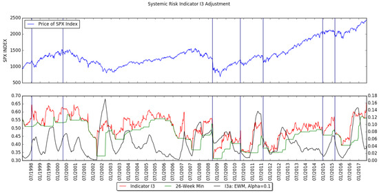
Figure 12.
Systemic Risk Indicator .
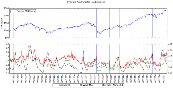
Figure 13.
Systemic Risk Indicator .
6.2. Square Wave Signal of Indicators
In electrical engineering, square wave form is very popular in digitalizing analog signal. Motivated by it, we transform our systemic risk indicators into square wave form in which high level signal represents financial crisis while low level one means healthy market. Figure 14 and Figure 15 show the square waves and that we convert from and respectively. Denote the up threshold as and the down threshold as . During the increasing and decreasing period of the indicators, we set high level if they increase to surpass for the first time and set low level if they decrease to cross for the first time.
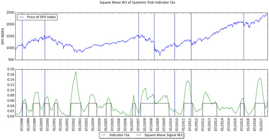
Figure 14.
Square Wave of Systemic Risk Indicator .
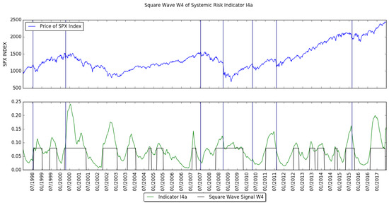
Figure 15.
Square Wave of Systemic Risk Indicator .
The choice of up and down thresholds is very important in converting the adjusted indicators and into square waves and , because it can also determine the time periods of the high and low levels within them, which eventually affects our trading strategies. However, after a large amount of tests, the threshold choices have a big range of values to make trading strategies outperform pure SPX Index investing, which means that the indicators are very applicable in avoiding financial crises. Here, we choose one set of threshold values:
to get square waves and and illustrate all of our following trading strategies in next subsection based on them.
Table 3 lists the financial drops including big crises and comparatively small drops and whether squared wave indicators can correctly predict them. Although they still have type I error in predicting crises, never miss any big one and even can cover some comparatively small drops in the market.
Table 3.
Financial Drops vs. Adjusted Indicators.
6.3. Validation by Trading Strategies
After obtaining the square wave forms of indicators, we develop some trading strategies of simple in-out, put protective and collar to validate our systemic risk indicators. For put protective, we design two strategies that put protective only indicators ring and put protective all the time. For collar, we implement three strategies that collar only indicators ring, collar all the time and covered call all the time but put protective only indicators ring.
In developing the SPX index investing with its options, we need to collect all the call and put options data with different maturities and moneynesses to calculate the implied volatility. We use the implied volatility data from SPX options with maturity of 1-month, 2-month, 3-month, 6-month and 12-month and moneynesses at 1.20, 1.10, 1.05, 1.025, 1, 0.975, 0.95, 0.90 and 0.80, and then interpolate the implied volatility through the smile curve when we need to buy or sell options which are then priced with Black Schole formula. Here, we set call options with moneynesses at 1.01 and put options at 0.99 in the following strategies and choose the yield of three-month treasury bill as the risk free interest rate.
In Figure 16 and Figure 17, we can see that except the put protective all the time and the collar all the time, all the strategies outperform the SPX index, which validates that our systemic risk indicators and are very competent in anticipating financial crises.
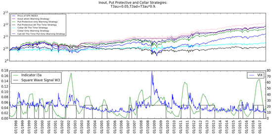
Figure 16.
In-out, Put Protective and Collar Strategies based on .
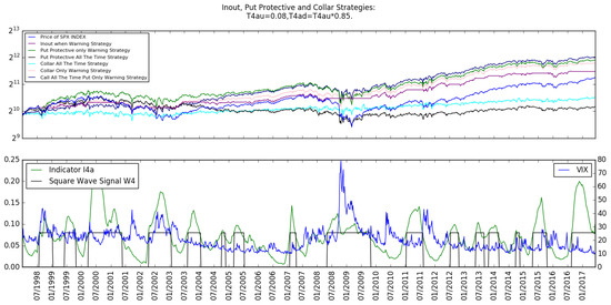
Figure 17.
In-out, Put Protective and Collar Strategies based on .
The indicators and do have several warning signals that the crisis actually does not come, but they never miss any big crisis from 1998 to 2017 and this type I error is acceptable based on the nice performances of our trading strategies. Therefore, they can be a very good tool for financial regulators and market professionals.
7. Conclusions
In this study, we firstly investigate systemic risk within financial network and establish a large set of market representative risk factors to describe the financial market as a holistic interconnected network system. We decompose the financial risk explained by each risk factor in the set into three independent components and aggregate them to propose our systemic risk indicators under the assumption that financial market is a stochastic process including the three independent levy processes.
Secondly, we illustrate the nonlinearity in the financial market by the simulation of temporal aggregation methodology with heavy-tailed distribution and real historical data plots. In addition, then we introduce our nonlinear PolyModel theory.
Then, we implement our theoretical ideas into empirical data and explore four systemic risk indicators, the former two of which are mainly seen as the trace of the evolution of financial crises while the latter two are considered as the early warning signals. In addition, the plots show that they are very effective in monitoring systemic risk and signaling early warnings of financial crises.
Finally, we develop some investing strategies of SPX index and its options based on two adjusted square wave form indicators to validate our results. The good performances of the strategies prove that our methodology of proposing systemic risk indicators is competent in monitoring market extreme downturns.
In sum, this study overcomes the defects that measuring systemic risk in an incomplete view of the market and with ideal linear risk models, and introduces a novel methodology to provide regulators and market professionals with additional helpful indicators in monitoring systemic risk and signaling early warnings of financial crises.
Author Contributions
Conceptualization, X.Y. and R.D.; Methodology, X.Y. and R.D.; Software, X.Y.; Validation, X.Y. and R.D.; Formal Analysis, X.Y.; Resources, X.Y.; Data Curation, X.Y.; Writing—Original Draft Preparation, X.Y.; Writing—Review and Editing, X.Y. and R.D.; Visualization, X.Y.; Supervision, X.Y. and R.D.; Project Administration, X.Y.
Funding
This research received no external funding.
Conflicts of Interest
All authors declare no conflict of interest. The opinions expressed in this paper are their individual one and does not represent the organizations/ academic institutions they are engaged with.
References
- Acemoglu, Daron, Asuman Ozdaglar, and Alireza Tahbaz-Salehi. 2015. Systemic risk and stability in financial networks. American Economic Review 105: 59–64. [Google Scholar] [CrossRef]
- Acharya, Viral, Lasse H. Pedersen, Thomas Philippon, and Matthew Richardson. 2010. Measuring systemic risk. The Review of Financial Studies 30: 2–47. [Google Scholar] [CrossRef]
- Acharya, Viral, Robert Engle, and Matthew Richardson. 2012. Capital shortfall: A new approach to ranking and regulating systemic risks. Journal of Econometrics 102: 59–64. [Google Scholar] [CrossRef]
- Adrian, Tobias, and Markus K. Brunnermeier. 2014. CoVaR. American Economic Review 106: 1705–41. [Google Scholar] [CrossRef]
- Armentia, Yannick, Stéphane Crépey, Samuel Drapeau, and Antonis Papapantoleon. 2015. Multivariate Shortfall Risk Allocation and Systemic Risk. Available online: https://arxiv.org/pdf/1507.05351 (accessed on 1 September 2017).
- Balla, Elian, Ibrahim Ergen, and Marco Migueis. 2014. Tail dependence and indicators of systemic risk for large US depositories. Journal of Financial Stability 15: 195–209. [Google Scholar] [CrossRef]
- Billio, Monica, Mila Getmansky, Andrew W. Lo, and Loriana Pelizzon. 2012. Econometric measures of connectedness and systemic risk in the finance and insurance sectors. Journal of Financial Economics 104: 535–59. [Google Scholar] [CrossRef]
- Blancher, Nicolas, Srobona Mitra, Hanan Morsy, A. Otani, Tiago Severo, and Laura Valderrama. 2013. Systemic Risk Monitoring (“SysMo”) Toolkit—A User Guide. IMF Working Paper: No.13/168. Washington, DC, USA: IMF. [Google Scholar]
- Brownlees, Christian, and Daniele Frison. 2014. How Interdependent Are Systemic Risk Indicators? Available online: https://www.jbs.cam.ac.uk/fileadmin/user_upload/research/centres/risk/downloads/140923_slides_brownlees.pdf (accessed on 11 August 2017).
- Brunnermeier, Markus K., and Patrick Cheridito. 2014. Measuring and Allocating Systemic Risk. Available online: https://ssrn.com/abstract=2372472 (accessed on 15 December 2017).
- Brunnermeier, Markus K., and Yuliy Sannikov. 2012. A macroeconomic model with a financial sector. America Economic Review 104: 379–421. [Google Scholar] [CrossRef]
- Chen, Zhou. 2010. Are banks too big to fail? Measuring systemic importance of financial institutions. International Journal of Central Banking 6: 205–50. [Google Scholar]
- Cherny, Alexander, Raphael Douady, and Stanislav Molchanov. 2010. On measuring nonlinear risk with scarce observations. Finance Stoch 14: 375–95. [Google Scholar] [CrossRef]
- Coste, Cyril, Raphael Douady, and Ilija I. Zovko. 2011. The Stress VaR: A new risk concept for extreme risk and fund allocation. The Journal of Alternative Investments 13: 10–23. [Google Scholar] [CrossRef]
- Dhillon, Paramveer S., Dean P. Foster, Sham M. Kakade, and Lyle H. Ungar. 2013. A risk comparison of ordinary least squares vs ridge regression. Journal of Machine Learning Research 14: 1505–11. [Google Scholar]
- Fabio, Caccioli, J. Doyne Farmer, Nick Foti, and Daniel Rockmore. 2015. Overlapping portfolios, contagion, and financial stability. Journal of Economic Dynamics and Control 51: 50–63. [Google Scholar]
- Glasserman, Paul, and H. Peyton Young. 2016. Contagion in financial networks. Journal of Economic Literature 54: 779–831. [Google Scholar] [CrossRef]
- Gray, Dale F. 2013. Modeling Banking, Sovereign, and Macro Risk in a CCA Global VAR. IMF Working Paper No. 13/218. Washington, DC, USA: IMF. [Google Scholar]
- Hansen, Lars Peter. 2013. Challenges in Identifying and Measuring Systemic Risk. University of Chicago Press Chapter in NBER book Risk Topography: Systemic Risk and Macro Modeling. Chicago: University of Chicago Press. [Google Scholar]
- Hartmann, Philipp, Kirstin Hubrich, Manfred Kremer, and Robert J. Tetlow. 2015. Melting Down: Systemic Financial Instability and the Macroeconomy. Available online: https://ssrn.com/abstract=2462567 (accessed on 11 August 2017).
- Huang, Xin, Hao Zhou, and Haibin Zhu. 2009. Systemic risk contributions. Journal of Financial Services Research 42: 55–83. [Google Scholar] [CrossRef]
- Hüser, Anne-Caroline. 2015. Too Interconnected to Fail: A Survey of the Interbank Networks Literature. SAFE Working Paper Series No.91. Frankfurt: Research Center SAFE—Sustainable Architecture for Finance in Europe. [Google Scholar]
- Langfield, Sam, and Kimmo Soramäki. 2014. Interbank exposure networks. Computational Economics 47: 3–17. [Google Scholar] [CrossRef]
- Markovic, Peta, and Branko Urošević. 2011. Market risk stress testing for internationally active financial institutions. Economic Annals 56: 188. [Google Scholar] [CrossRef]
- Moore, Kyle, and Chen Zhou. 2012. Identifying Systemically Important Financial Institutions: Size and Other Determinants. Available online: https://papers.ssrn.com/sol3/papers.cfm?abstract_id=2104145 (accessed on 22 April 2018).
- Patro, Dilip K., Min Qi, and Xian Sun. 2013. A simple indicator of systemic risk. Journal of Financial Stability 9: 105–16. [Google Scholar] [CrossRef]
- Rama Cont, Amal Moussa, and Andreea Minca. 2009. Too Interconnected to Fail: Contagion and Systemic Risk in Financial Networks. Lecture presented at the IMF. New York: Columbia University. [Google Scholar]
- Raphael, Douady, and Ilija I. Zovko. 2014. Polymodels and their application in portfolio risk. In Laboratory of Excellence on Financial Regulation (Labex ReFi). Supported by PRES heSam under the Reference ANR-10-LABX-0095. Paris: Laboratory of Excellence on Financial Regulation. [Google Scholar]
- Schwaab, Bernd, Siem Jan Koopman, and Andre Lucas. 2011. Systemic Risk Diagnostic: Coincident Indicators and Early Warning Signals. Euro Central Bank Working Paper No.1327. Frankfurt, Germany: European Central Bank. [Google Scholar]
- Sorkin, Andrew Ross, and William Hughes. 2009. Too Big to Fail. New York: Penguin Audio. [Google Scholar]
- Sornette, Didier, and Anders Johansen. 1997. Large financial crashes. Physica A 245: 411–22. [Google Scholar] [CrossRef]
- Sornette, Didier, and Anders Johansen. 2001. Significance of log-periodic precursors to financial crashes. Quantitative Finance 1: 452–71. [Google Scholar] [CrossRef]
- Sornette, Didier, and Jonas Valbjørn Anderson. 2002. A nonlinear super-exponential rational model of speculative financial bubbles. International Journal of Modern Physics A 13: 171. [Google Scholar] [CrossRef]
- Sornette, Didier, Anders Johansen, and Jean-Philippe Bouchaud. 1996. Stock market crashes, precursors and replicas. Journal de Physique I France 6: 167–75. [Google Scholar] [CrossRef]
- Sornette, Didier, and Wei-Xing Zhou. 2006. Predictability of large future changes in major financial indices. International Journal of Forecasting 22: 153–68. [Google Scholar] [CrossRef]
- Stoyanov, Stoyan. 2016. Pitfalls of linear risk assessment. Paper Presented at the Real World Risk Institute Conference, New York, NY, USA, February 13. [Google Scholar]
- Stoyanov, Stoyan V., Svetlozar T. Rachev, Boryana Racheva-Iotova, and Frank J. Fabozzi. 2010. Fat-Tailed Models for Risk Estimation. Journal of Portfolio Management. Available online: https://ssrn.com/abstract=1729040 (accessed on 12 September 2017).
© 2018 by the authors. Licensee MDPI, Basel, Switzerland. This article is an open access article distributed under the terms and conditions of the Creative Commons Attribution (CC BY) license (http://creativecommons.org/licenses/by/4.0/).