Forecasting of Realised Volatility with the Random Forests Algorithm


Abstract
1. Introduction
2. Materials and Methods
2.1. Random Forests Algorithm
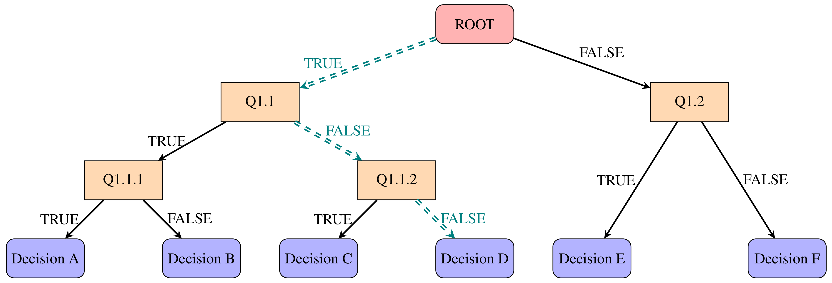
2.1.1. Decision Trees
- Root nodes: entry points to a collection of data;
- Inner nodes: a set of binary questions where each child node is available for every possible answer;
- Leaf nodes: respond to the decision to take if reached.
| Algorithm 1: Classification And Regression Trees - CART algorithm for building decision trees. |
| 1: Let N be the root node with all available data. |
| 2: Find the feature F and threshold value T that split the samples assigned to N into subsets |
| and , to maximise the label purity within these subsets. |
| 3: Assign the pair (F, T) to N. |
| 4: If is too small to be split, attach a ‘child’ leaf node to and to N and |
| assign the leaves with the most present label in and , respectively. |
| If subset is large enough to be split, attach child nodes and to N, |
| and then assign to them, respectively. |
| 5: Repeat steps 2–4 for the new nodes and until the new subsets |
| can no longer be split. |
2.1.2. Random Forests
| Algorithm 2: Random forests |
| 1: Draw a number of bootstrap samples from the original data () to be grown. |
| 2: Sample N cases at random with replacement to create a subset of the data. The subset is |
| then split into in-bag and out-of-bag samples at a selected ratio (i.e., 7:3). |
| 3: At each node, for a preselected number m, m predictor variables () are chosen at |
| random from all the predictor variables. |
| 4: The predictor variable that provides the best split, according to some objective function, |
| is used to build a binary split on that node. |
| 5: At the next node, choose another m variables at random from all predictor variables. |
| 6: Repeat 3–5 until all nodes are grown. |
2.2. Volatility Measures
2.2.1. Realised Volatility
2.2.2. The Purified Implied Volatility
2.3. Models for Volatility
2.3.1. Heterogeneous Autoregressive Model for Realised Volatility
2.4. The Modified HAR Model for Realised Volatility and Forecasting the Direction
- The Average True Range (ATR): The ATR is an indicator that measures volatility by using the high–low range of the daily prices. ATR is based on n-periods and can be calculated on an intraday, daily, weekly, or monthly basis. It is noted that ATR is often used as a proxy for volatility. To estimate , we are required to compute the “true range” (TR) such thatwhere , , are the current highest return, the current lowest return, and the previous last return of a selected period, respectively, with absolute values to ensure is always positive. Hence, the average true range within n-days is
- Close Relative To Daily Range (CRTDR): The location of the last return within the day’s range is a powerful predictor of next-returns. Here, CRTDR is estimated bywhere, , and are the high, low, and close returns at time for a selected time period using high frequency returns.
- Exponential Moving Average of realised volatility (EMARV): Exponential moving averages reduce the lag effect in time-series by applying more weight to recent prices. The weighting applied to the most recent price depends on the number of periods (n) in the moving average and the weighting multiplier (). The formula for EMARV of n-periods is as follows:
- Moving average convergence/divergence oscillator (MACD) measure of realised volatility: The MACD is one of the simplest and most effective momentum indicators. It turns two moving averages into a momentum oscillator by subtracting the longer moving average (m-days) from the shorter moving average (n-days). The MACD fluctuates above and below the zero line as the moving averages converge, cross, and diverge. We estimate the MACD for realised volatility as
- Relative Strength Index for realised volatility (RSIRV): This is also a momentum oscillator that measures the speed and change of volatility movements. We define RSIRV aswhere is the average increase in volatility and is the average decrease in volatility within n-days.
| Algorithm 3: Forecasting the direction of realised volatility |
| 1: Obtain the direction of the realised volatility. |
| 2: Compute the above technical indicators for each observation. |
| 3: Split the data into a training set and a testing set. |
| 4: Apply the random forests algorithm to the training set to develop the pattern solution of |
| the realised volatility using the above indicators. |
| 5: Use the solution from Step 4 to predict the direction of the testing set. |
2.5. Forecasting the Realised Volatility—The Proposed Model
3. The results
3.1. Measuring Errors
3.1.1. Classification Problem
- True positive (TP): The number of days that are observed with “DOWN” signals that were correctly predicted.
- False positive (FP): The number of days that are observed with “DOWN” signals that were predicted to have “UP” signals.
- False negative (FN): The number of days that are observed with “UP” signals that were predicted to have “DOWN” signals.
- True negative (TN): The number of days that are observed with “UP” signals that were correctly predicted.
- Accuracy: the proportion of the total number of correct predictions
3.1.2. Regression Problem
- For each bootstrap, predict the out-of-bag values using the tree grown within the bootstrap sample.
- Aggregate the Out-of-bag (OOB) predictions and calculate the mean square error rate bywhere m is the number of observations in the OOB data (i.e., ) and is the average of the OOB predictions for the observation.
- Estimate the percentage variance explained as a measure of goodness of fit bywhere is the variance in the OOB sample.
- The mean absolute error
- The mean absolute percentage error
- The root mean square error
- The root mean square percentage error
3.2. Empirical Results
3.2.1. Data Description
3.2.2. The Results
4. Discussion
5. Conclusions
Author Contributions
Funding
Conflicts of Interest
References
- Andersen, Torben G., and Tim Bollerslev. 1997. Heterogeneous information arrivals and return volatility dynamics: Uncovering the long run in high frequency data. Journal of Finance 52: 975–1005. [Google Scholar] [CrossRef]
- Andersen, Torben G., Tim Bollerslev, Francis X. Diebold, and Paul Labys. 2003. Modeling and forecasting realized volatility. Econometrica 71: 529–626. [Google Scholar] [CrossRef]
- Barndorff-Nielsen, Ole E., and Neil Shephard. 2001. Econometric Analysis of Realised Volatility and its Use in Estimating Stochastic Volatility Models. Journal of the Royal Statistical Society 64: 253–80. [Google Scholar] [CrossRef]
- Barndorff-Nielsen, Ole E., and Neil Shephard. 2004. Power and bipower variation with stochastic volatility and jumps. Journal of Financial Econometrics 2: 1–37. [Google Scholar] [CrossRef]
- Black, Fischer, and Myron Scholes. 1973. The Pricing of Options and Corporate Liabilities. Journal of Political Economy 81: 637–54. [Google Scholar] [CrossRef]
- Black, Fischer. 1976. The pricing of commodity contracts. Journal of Financial Economics 3: 167–79. [Google Scholar] [CrossRef]
- Bollerslev, Tim. 1986. Generalized Auto Regressive Conditional Heteroskedasticity. Journal of Econometrics 31: 307–27. [Google Scholar] [CrossRef]
- Breiman, Leo, J. H. Friedman, R. A. Olshen, and C. J. Stone. 1984. Classification and Regression Trees. Monterey: Wadsworth and Brooks. [Google Scholar]
- Breiman, Leo. 2001. Random Forests. Machine Learning 45: 5–32. [Google Scholar] [CrossRef]
- Carr, Peter, and Liuren Wu. 2006. A tale of two indices. Journal of Derivatives 3: 13–29. [Google Scholar] [CrossRef]
- Corsi, Fulvio, and Roberto Reno. 2009. HAR Volatility Modelling With Heterogeneous Leverage and Jumps. Available online: https://web.stanford.edu/group/SITE/archive/SITE_2009/segment_1/s1_papers/corsi.pdf (accessed on 10 October 2018).
- Corsi, Fulvio. 2003. A Simple Approximate Long-Memory Model of Realized Volatility. Journal of Financial Econometrics 7: 174–96. [Google Scholar] [CrossRef]
- De Stefani, Jacopo, Olivier Caelen, Dalila Hattab, and Gianluca Bontempi. 2017. Machine Learning for Multi-step Ahead Forecasting of Volatility Proxies. Available online: https://pdfs.semanticscholar.org/39cf/3536e780ff195d400902076e1b3e7b2e638d.pdf (accessed on 20 September 2015).
- Dokuchaev, Nikolai. 2014. Volatility estimation from short time series of stock prices. Journal of Nonparametric Statistics 26: 373–84. [Google Scholar] [CrossRef]
- Engle, Robert F. 1982. Autoregressive conditional heteroskedasticity with estimates of variance of UK inflation. Econometrica 50: 987–1008. [Google Scholar] [CrossRef]
- Engle, Robert F. 1990. Discussion: Stock market volatility and the crash of 87. Review of Financial Studies 3: 103–6. [Google Scholar] [CrossRef]
- Glosten, Lawrence R., Ravi Jagannathan, and David E. Runkle. 1993. On the relationship between the expected value and the volatility of the nominal excess return on stocks. Journal of Finance 46: 1779–801. [Google Scholar] [CrossRef]
- Heston, Steven L. 1993. A closed-form solution for options with stochastic volatility with applications to bond and currency options. The Review of Financial Studies 6: 327–43. [Google Scholar] [CrossRef]
- Khan, Md Ashraful Islam. 2011. Financial Volatility Forecasting by Nonlinear Support Vector Machine Heterogeneous Autoregressive Model: Evidence from Nikkei 225 Stock Index. International Journal of Economics and Finance 3: 138–50. [Google Scholar] [CrossRef]
- Luong, Chuong, and Nikolai Dokuchaev. 2014. Analysis of market volatility via a dynamically purified option price process. Annals of Financial Economics 9: 1450006. [Google Scholar] [CrossRef]
- Luong, Chuong, and Nikolai Dokuchaev. 2016. Modelling dependency of volatility on sampling frequency via delay equations. Annals of Financial Economics 11: 1650007. [Google Scholar] [CrossRef]
- Lux, Thomas, and Michele Marchesi. 1999. Scaling and criticality in a stochastic multi-agent model of financial market. Nature 397: 498–500. [Google Scholar] [CrossRef]
- Müller, Ulrich A., Michel M. Dacorogna, Rakhal D. Davé, Richard B. Olsen, Olivier V. Pictet, and Jacob E. Von Weizsäcker. 1997. Volatilities of different time resolutions: Analyzing the dynamics of market components. Journal of Empirical Finance 4: 213–39. [Google Scholar] [CrossRef]
- Nelson, Daniel B. 1991. Conditional Heteroskedasticity in Asset Returns: A New Approach. Econometrica 59: 347–70. [Google Scholar] [CrossRef]
- Peters, Edgar. 1994. Fractal Market Analysis. In A Wiley Finance Edition. New York: John Wiley & Sons. [Google Scholar]
- Qin, Qin, Qing-Guo Wang, Jin Li, and Shuzhi Sam Ge. 2013. Linear and Nonlinear Trading Models with Gradient Boosted Random Forests and Application to Singapore Stock Market. Journal of Intelligent Learning Systems and Applications 5: 1–10. [Google Scholar] [CrossRef]
- Reuters, Thomson. 2015. Thomson Reuters Tick History. Available online: http://www.sirca.org.au/ (accessed on 20 September 2015).
- Theofilatos, Konstantinos, Spiros Likothanassis, and Andreas Karathanasopoulos. 2012. Modeling and Trading the EUR/USD Exchange Rate Using Machine Learning Techniques. ETASR—Engineering, Technology & Applied Science Research 2: 269–72. [Google Scholar]
- Whaley, Robert E. 2000. The investor fear gauge. The Journal of Portfolio Management 6: 12–17. [Google Scholar] [CrossRef]
- Zakoian, Jean-Michel. 1994. Threshold Heteroscedastic Models. Journal of Economic Dynamics and Control 18: 931–55. [Google Scholar] [CrossRef]


| Series | Mean | Std. Dev. | Skew. | Kurt. | Min. | Max. | PV | |||
| 0.1335 | 0.0848 | 2.4957 | 8.9530 | 0.0328 | 0.7811 | 1 | 0.8441 | 0.7523 | 0.7757 | |
| 0.1335 | 0.0721 | 2.0481 | 5.4748 | 0.0484 | 0.5453 | 0.8441 | 1 | 0.9042 | 0.8919 | |
| 0.1331 | 0.0664 | 1.8304 | 3.9311 | 0.0593 | 0.4228 | 0.7523 | 0.9042 | 1 | 0.9180 | |
| PV | 0.1614 | 0.0705 | 1.5181 | 2.8461 | 0.0698 | 0.5004 | 0.7757 | 0.8919 | 0.9180 | 1 |
| Series | Mean | Std. Dev | Skew. | Kurt. | Min. | Max. | ||||
| −2.1588 | 0.5139 | 0.5678 | 0.2336 | −3.4184 | −0.2471 | 1 | 0.8548 | 0.7739 | 0.7936 | |
| −2.1244 | 0.4499 | 0.6619 | 0.0960 | −3.0274 | −0.6064 | 0.8548 | 1 | 0.9124 | 0.8972 | |
| −2.113 | 0.4213 | 0.7156 | −0.0407 | −2.8248 | −0.8608 | 0.7739 | 0.9124 | 1 | 0.9017 | |
| −1.9044 | 0.3893 | 0.5190 | −0.3229 | −2.6618 | −0.6923 | 0.7936 | 0.8972 | 0.9017 | 1 |
| 1-Day | 5-Day | 22-Day | |||||||||||
|---|---|---|---|---|---|---|---|---|---|---|---|---|---|
| HAR-JL | HAR-JL-PV | HAR-JL-D | HAR-JL-PV-D | HAR-JL | HAR-JL-PV | HAR-JL-D | HAR-JL-PV-D | HAR-JL | HAR-JL-PV | HAR-JL-D | HAR-JL-PV-D | ||
| RV | RMSE | 0.0031 | 0.0029 | 0.0018 | 0.0018 | 0.002 | 0.0011 | 0.0010 | 0.0010 | 0.0011 | 0.0010 | 0.0009 | 0.0001 |
| % OOB Var | 57.81 | 59.61 | 74.68 | 75.58 | 79.28 | 80.28 | 81.13 | 81.81 | 74.47 | 76.44 | 78.09 | 79.44 | |
| log RV | RMSE | 0.0996 | 0.0957 | 0.0509 | 0.0502 | 0.0378 | 0.0336 | 0.0326 | 0.0295 | 0.0383 | 0.0323 | 0.0339 | 0.0287 |
| % OOB Var | 61.66 | 63.12 | 80.39 | 80.65 | 80.55 | 82.70 | 83.25 | 84.83 | 77.48 | 81.97 | 80.05 | 83.12 | |
| 1-Day | 5-Day | 22-Day | |||||||||||
|---|---|---|---|---|---|---|---|---|---|---|---|---|---|
| HAR-JL | HAR-JL-PV | HAR-JL-D | HAR-JL-PV-D | HAR-JL | HAR-JL-PV | HAR-JL-D | HAR-JL-PV-D | HAR-JL | HAR-JL-PV | HAR-JL-D | HAR-JL-PV-D | ||
| RV | MAE | 0.0212 | 0.0205 | 0.0176 | 0.0171 | 0.0147 | 0.0135 | 0.0137 | 0.0127 | 0.0184 | 0.0142 | 0.017 | 0.0137 |
| MAPE | 0.2715 | 0.2516 | 0.2042 | 0.1974 | 0.1814 | 0.1573 | 0.1670 | 0.1500 | 0.2245 | 0.1630 | 0.2094 | 0.1576 | |
| RMSE | 0.0285 | 0.0277 | 0.0247 | 0.0235 | 0.0192 | 0.0182 | 0.0180 | 0.0168 | 0.0223 | 0.0182 | 0.0209 | 0.0176 | |
| RMSPE | 0.3610 | 0.3245 | 0.2709 | 0.2568 | 0.2352 | 0.2025 | 0.2181 | 0.1926 | 0.2745 | 0.2046 | 0.2602 | 0.1973 | |
| log RV | MAE | 0.0206 | 0.0201 | 0.0170 | 0.0165 | 0.0143 | 0.0135 | 0.0130 | 0.0129 | 0.0170 | 0.0138 | 0.0156 | 0.0135 |
| MAPE | 0.2525 | 0.2331 | 0.1947 | 0.1878 | 0.1740 | 0.1553 | 0.1574 | 0.1481 | 0.2058 | 0.1576 | 0.1881 | 0.1532 | |
| RMSE | 0.0279 | 0.0280 | 0.0239 | 0.0233 | 0.0185 | 0.0185 | 0.0175 | 0.0175 | 0.0206 | 0.0177 | 0.0191 | 0.0174 | |
| RMSPE | 0.3250 | 0.2929 | 0.2573 | 0.2454 | 0.2230 | 0.1980 | 0.2116 | 0.1913 | 0.2499 | 0.1958 | 0.2310 | 0.1912 | |
© 2018 by the authors. Licensee MDPI, Basel, Switzerland. This article is an open access article distributed under the terms and conditions of the Creative Commons Attribution (CC BY) license (http://creativecommons.org/licenses/by/4.0/).
Share and Cite
Luong, C.; Dokuchaev, N. Forecasting of Realised Volatility with the Random Forests Algorithm. J. Risk Financial Manag. 2018, 11, 61. https://doi.org/10.3390/jrfm11040061
Luong C, Dokuchaev N. Forecasting of Realised Volatility with the Random Forests Algorithm. Journal of Risk and Financial Management. 2018; 11(4):61. https://doi.org/10.3390/jrfm11040061
Chicago/Turabian StyleLuong, Chuong, and Nikolai Dokuchaev. 2018. "Forecasting of Realised Volatility with the Random Forests Algorithm" Journal of Risk and Financial Management 11, no. 4: 61. https://doi.org/10.3390/jrfm11040061
APA StyleLuong, C., & Dokuchaev, N. (2018). Forecasting of Realised Volatility with the Random Forests Algorithm. Journal of Risk and Financial Management, 11(4), 61. https://doi.org/10.3390/jrfm11040061