Nonlinear Time Series Modeling: A Unified Perspective, Algorithm and Application

Abstract

A new comprehensive approach to nonlinear time series analysis and modeling is developed in the present paper. We introduce novel data-specific mid-distribution-based Legendre Polynomial (LP)-like nonlinear transformations of the original time series $\left\{Y\right(t\left)\right\}$ that enable us to adapt all the existing stationary linear Gaussian time series modeling strategies and make them applicable to non-Gaussian and nonlinear processes in a robust fashion. The emphasis of the present paper is on empirical time series modeling via the algorithm LPTime. We demonstrate the effectiveness of our theoretical framework using daily S&P 500 return data between 2 January 1963 and 31 December 2009. Our proposed LPTime algorithm systematically discovers all the ‘stylized facts’ of the financial time series automatically, all at once, which were previously noted by many researchers one at a time.

1. Introduction

When one observes a sample $Y\left(t\right),t=1,\dots ,T$, of a (discrete parameter) time series $Y\left(t\right)$, one seeks to nonparametrically learn from the data a stochastic model with two purposes: (a1) scientific understanding; (a2) forecasting (predict future values of the time series under the assumption that the future obeys the same laws as the past). Our prime focus in this paper is on developing a nonparametric empirical modeling technique for nonlinear (stationary) time series that can be used by data scientists as a practical tool for obtaining insights into (i) the temporal dynamic patterns and (ii) the internal data generating mechanism; a crucial step for achieving (a1) and (a2).

Under the assumption that the time series is stationary (which can be extended to asymptotically stationary), the distribution of $Y\left(t\right)$ is identical for all t, and the joint distribution of $Y\left(t\right)$ and $Y(t+h)$ depends only on lag h. Typical estimation goals are as follows:

(1)

Marginal modeling: The identification of the marginal probability law (in particular, the heavy-tailed marginal densities) of a time series plays a vital role in financial econometrics. Notations: common quantile Q, inverse of the distribution function F, respectively denoted $Q(u;Y),0<u<1$ and $F(y;Y)$. The mid-distribution is defined as $F^{\mathrm{mid}}(y;Y)=F(y;Y)-0.5\mathrm{Pr}(Y\left(t\right)=y)$.

(2)

Correlation modeling: Covariance function (defined for positive and negative lag h) $R(h;Y)=\mathrm{Cov}\left[Y\right(t),Y(t+h\left)\right]$. $R(0;Y)=\mathrm{Var}\left[Y\right(t\left)\right]$, $\mu =\mathbb{E}\left[Y\right(t\left)\right]$ assumed zero in our prediction theory. Correlation function $\rho \left(h\right)=\mathrm{Cor}\left[Y\right(t),Y(t+h\left)\right]=R(h;Y)/R(0;Y)$.

(3)

Frequency-domain modeling: When covariance is absolutely summable, define spectral density function $f(\omega ;Y)=\sum R(h;Y)e^{-2\pi i\omega h},-1/2<\omega <1/2$.

(4)

Time-domain modeling: The time domain model is a linear filter relating $Y\left(t\right)$ to white noise $ϵ\left(t\right)$, $\mathcal{N}(0,1)$ independent random variables. Autoregressive scheme of order m, a predominant linear time series technique for modeling conditional mean, is defined as (assuming $\mathbb{E}\left[Y\right(t\left)\right]=0$):

$$Y\left(t\right)-a(1;m)Y(t-1)-\dots -a(m;m)Y(t-m)={\sigma }_mϵ\left(t\right),$$

(1)

with the spectral density function given by:

$$f(\omega ;Y)={\displaystyle \frac{{\sigma }_m^2}{|1-{\sum }_{k=1}^{m}a(k;m)e^{2\pi i\omega k}{|}^2}}.$$

(2)

To fit an AR model, compute the linear predictor of $Y\left(t\right)$ given $Y(t-j),j=1,\dots ,m$ by:

$$Y^{\mu ,m}\left[t\right]=\mathbb{E}\left[Y\left(t\right)\mid Y(t-1),\dots ,Y(t-m)\right]=a(1;m)Y(t-1)+\cdots +a(m;m)Y(t-m).$$

(3)

Verify that the prediction error $Y\left[t\right]-Y^{\mu ,m}\left[t\right]$ is white noise. The best fitting AR order is identified by the Akaike criterion (AIC) (or Schwarz’s criterion, BIC) as the value of m minimizes:

$$\mathrm{AIC}\left(m\right)=2\log {\sigma }_m+2m/n.$$

In what follows, we aim to develop a parallel modeling framework for nonlinear time series.

2. From Linear to Nonlinear Modeling

Our approach to nonlinear modeling, called LPTime1, is via approximate calculation of conditional expectation $\mathbb{E}\left[Y\right(t\left)\right|Y(t-1),\dots ,Y(t-m)]$. Because with probability one $Q\left(F\right(Y\left)\right)=Y$, one can prove that the conditional expectation of $Y\left(t\right)$ given past values $Y(t-j)$ is equal to (with probability one) the conditional expectation of $Y\left(t\right)$ given past values $F^{\mathrm{mid}}\left(Y(t-j)\right)$, which can be approximated by linear orthogonal series expansion in score functions $T_k\left[F^{\mathrm{mid}}\left(Y(t-j)\right)\right]$ constructed by Gram–Schmidt orthonormalization of powers of:

$$T_1={\displaystyle \frac{F^{\mathrm{mid}}(Y\left(t\right);Y)-0.5}{\sigma \left[F^{\mathrm{mid}}(Y\left(t\right);Y)\right]}},$$

(4)

where $\sigma \left[F^{\mathrm{mid}}(Y\left(t\right);Y)\right]$ is the standard deviation of the mid-distribution transform random variable given by $\sqrt{(1-{\sum }_y{p}^3\left(y\right))/12}$ and $p\left(y\right)$ denotes the probability mass function of Y. This score polynomial allows us to simultaneously tackle the discrete (say count-valued) and continuous time series. Note that for Y continuous, $T_1$ reduces to:

$$T_1=\sqrt{12}\left(F\left(Y\right(t\left)\right)-0.5\right).$$

(5)

and all the higher order polynomials $T_j$ can be compactly expressed as ${\mathrm{Leg}}_j\left[F\left(Y\right)\right]$, where ${\mathrm{Leg}}_j\left(u\right),0<u<1$ denotes orthonormal Legendre polynomials. It is worthwhile to note that $T_j$ are orthonormal polynomials of mid-rank (instead of polynomials of the original y’s), which inject robustness into our analysis while allowing us to capture nonlinear patterns. Having constructed score functions of y denoted by $T_j$, we transform it into a unit interval by letting $y=Q(u;Y)$ and defining:

$$S_j(u;Y)=T_j\left[F^{\mathrm{mid}}\left(Q(u;Y)\right)\right],T_j(y;Y)=S_j\left[F^{\mathrm{mid}}\left(Y\left(t\right)\right)\right].$$

(6)

In general, our score functions are custom constructed for each distribution function F, which can be discrete or continuous.

3. Nonparametric LPTime Analysis

Our LPTime empirical time series modeling strategy for nonlinear modeling of a univariate time series $Y\left(t\right)$ is based on linear modeling of the multivariate time series:

$$\mathrm{Vec}\left(\mathrm{YS}\right)\left(t\right)={\left[{\mathrm{YS}}_1\left(t\right),\dots ,{\mathrm{YS}}_k\left(t\right)\right]}^{\mathrm{T}},$$

(7)

where ${\mathrm{YS}}_k\left(t\right)=T_k\left[F^{\mathrm{mid}}\left(Y\left(t\right)\right)\right]$, our tailor-made orthonormal mid-rank-based nonlinear transformed series. We summarize below the main steps of the algorithm LPTime. To better understand the functionality and applicability of LPTime, we break it into several inter-connected steps, each of which highlights:

(a)

The algorithmic modeling aspect (how it works).

(b)

The required theoretical ideas and notions (why it works).

(c)

The application to daily S&P 500 return data between 2 January 1963 and 31 December 2009 (empirical proof-of-work).

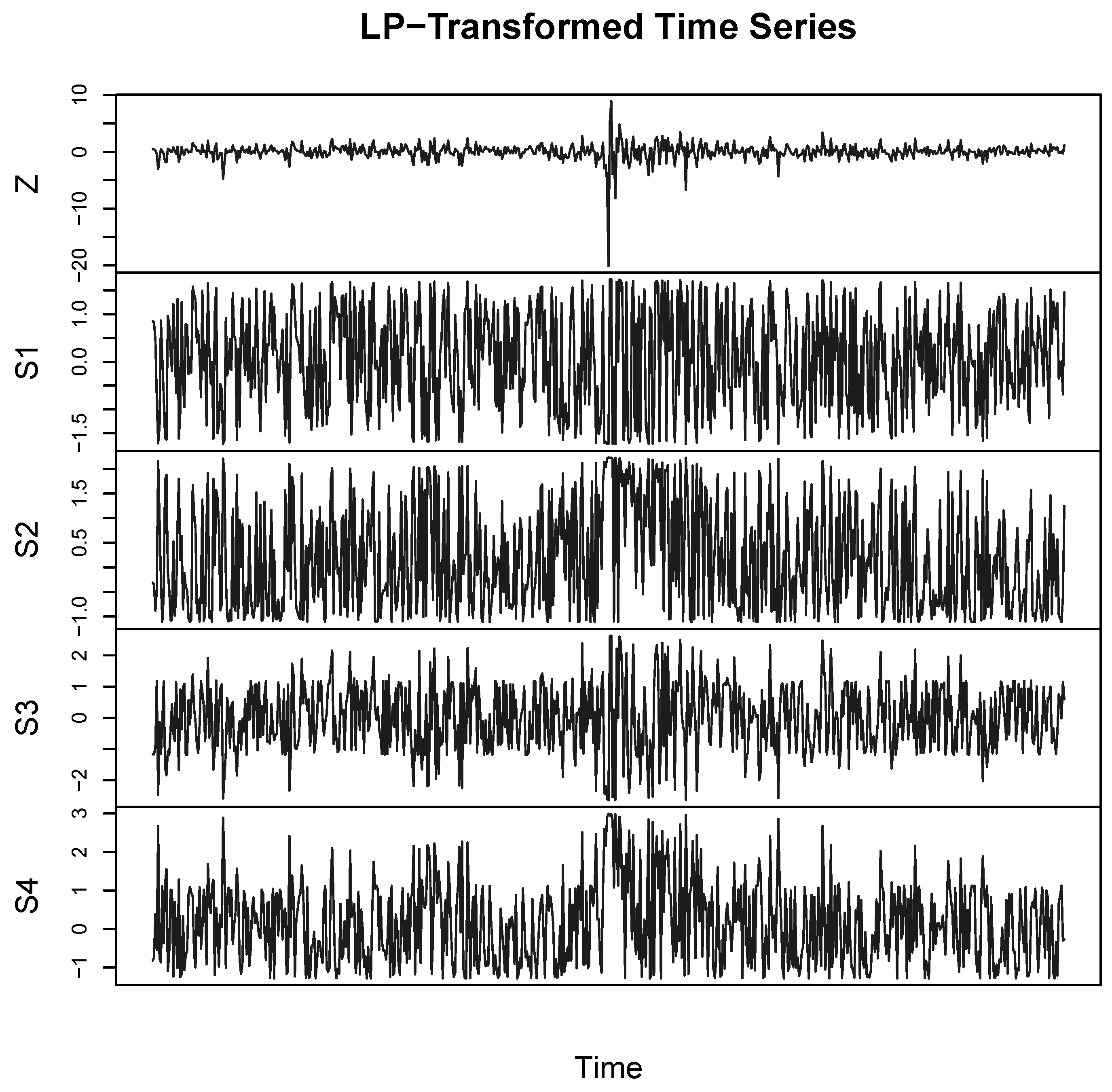
3.1. The Data and LP-Transformation

The data used in this paper are daily S&P 500 return data between 2 January 1963 and 31 December 2009 (defined as $\log (P_t/P_{t-1})$, where $P_t$ is the closing price on trading day t). We begin our modeling process by transforming the given univariate time series $\left\{Y\right(t\left)\right\}$ into multiple (robust) time series by means of special data-analytic construction rules described in Equations (4)–(6) and (7). We display the original “normalized” time series $\mathcal{Z}\left(Y\right(t\left)\right)=\left(Y\right(t)-\mathbb{E}[Y\left(t\right)\left]\right)/\sigma \left[Y\right(t\left)\right]$ and the transformed time series ${\mathrm{YS}}_1\left(t\right),\dots ,{\mathrm{YS}}_k\left(t\right)$ on a single plot.

Figure 1 shows the first look at the transformed S&P 500 return data between October 1986 and October 1988. These newly-constructed time series work as a universal preprocessor for any time series modeling in contrast with other ad hoc power transformations. In the next sections, we will describe how the temporal patterns of these multivariate LP-transformed series $\mathrm{Vec}\left(\mathrm{YS}\right)\left(t\right)=\{{\mathrm{YS}}_1\left(t\right),\dots ,{\mathrm{YS}}_k\left(t\right)\}$ generate various insights for the time series $\left\{Y\right(t\left)\right\}$ in an organized fashion.

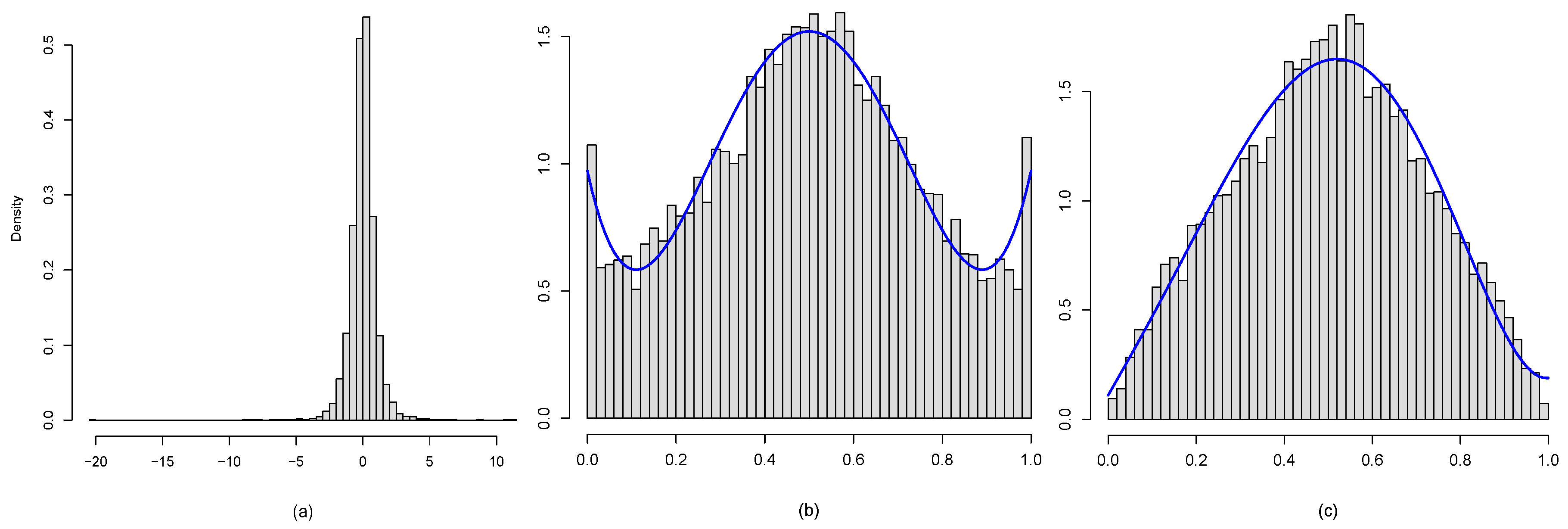
3.2. Marginal Modeling

Our time series modeling starts with the nonparametric identification of probability distributions.

Non-Normality Diagnosis

Does the normal probability distribution provide a good fit to the S&P 500 return data? Figure 2a clearly indicates that the distribution of daily return is certainly non-normal. At this point, the natural question is how the distribution is different from the assumed normal one? A quick insight into this question can be gained by looking at the distribution of the random variable $U=G\left(Y\right)$, called the comparison density (Mukhopadhyay 2017; Parzen 1997), given by:

$$d(u;G,F)={\displaystyle \frac{f\left(Q\right(u;G\left)\right)}{g\left(Q\right(u;G\left)\right)}},0\le u\le 1,$$

(8)

where $Q(u;G)=\inf \{x:G(x)\ge u\}$ is the quantile function. The flat uniform shape of the estimated comparison density provides a quick graphical diagnostic to test the fit of the parametric G to the true unknown distribution F. The Legendre polynomial-based orthogonal series comparison density estimator is given by:

$$d(u;G,F)=1+\sum _j\mathrm{LP}[j;G,F]{\mathrm{Leg}}_j\left(u\right),0<u<1$$

(9)

where the Fourier coefficients $\mathrm{LP}[j;G,F]=\mathbb{E}[{\mathrm{Leg}}_j\circ G\left(Y\right)]$.

For $G=\Phi$, Figure 2b displays the histogram of $U_i=\Phi \left(Y_i\right)$ for $i=1,\dots ,n$. The corresponding comparison density estimate $\widehat{d}(u;G,F)=1-0.271{\mathrm{Leg}}_2\left(u\right)-0.021{\mathrm{Leg}}_3\left(u\right)+0.193{\mathrm{Leg}}_4\left(u\right)$ is shown with the blue curve, which reflects the fact that the distribution of daily return (i) has a sharp peaked (inverted “U” shape) and (ii) is negatively skewed with (iii) fatter tails than the Gaussian distribution. We can carry out a similar analysis by asking whether the t-distribution with two degrees of freedom provides a better fit. Figure 2c demonstrates the full analysis, where the estimated comparison density $\widehat{d}(u;G,F)=1-0.492{\mathrm{Leg}}_2\left(u\right)-0.015{\mathrm{Leg}}_3\left(u\right)+0.084{\mathrm{Leg}}_4\left(u\right)$ indicates that (iv) the t-distribution fits the data better than normal, especially in the tails, although not a fully-adequate model.

The shape of the comparison density (along with the histogram of $U_i=G\left(Y_i\right)$, $i=1,\dots ,n$) captures and exposes the adequacy of the assumed model G for the true unknown F; thus acting as an exploratory, as well as confirmatory tool.

3.3. Copula Dependence Modeling

Distinguishing uncorrelatedness and independence by properly quantifying association is an essential task in empirical nonlinear time series modeling.

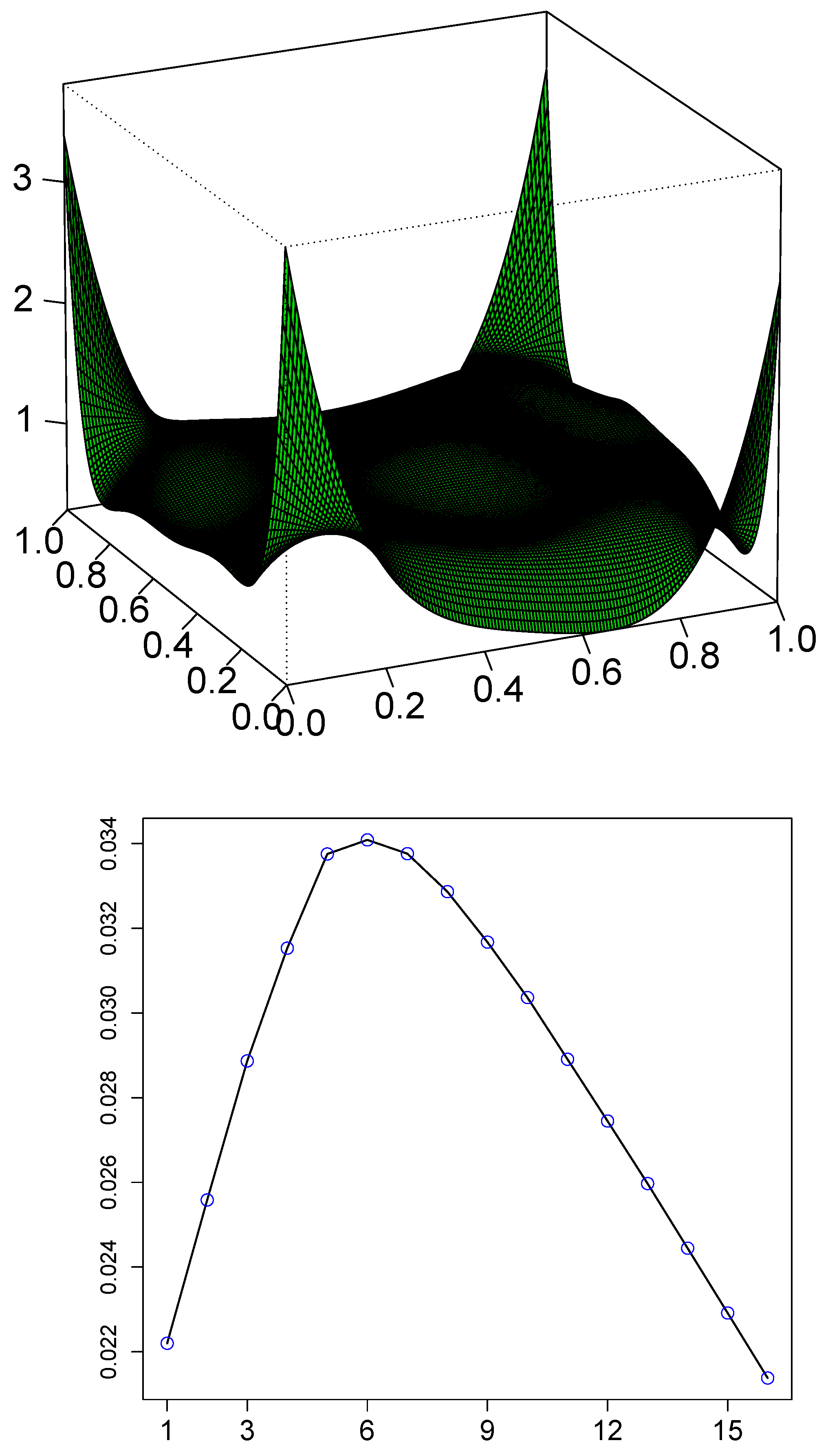
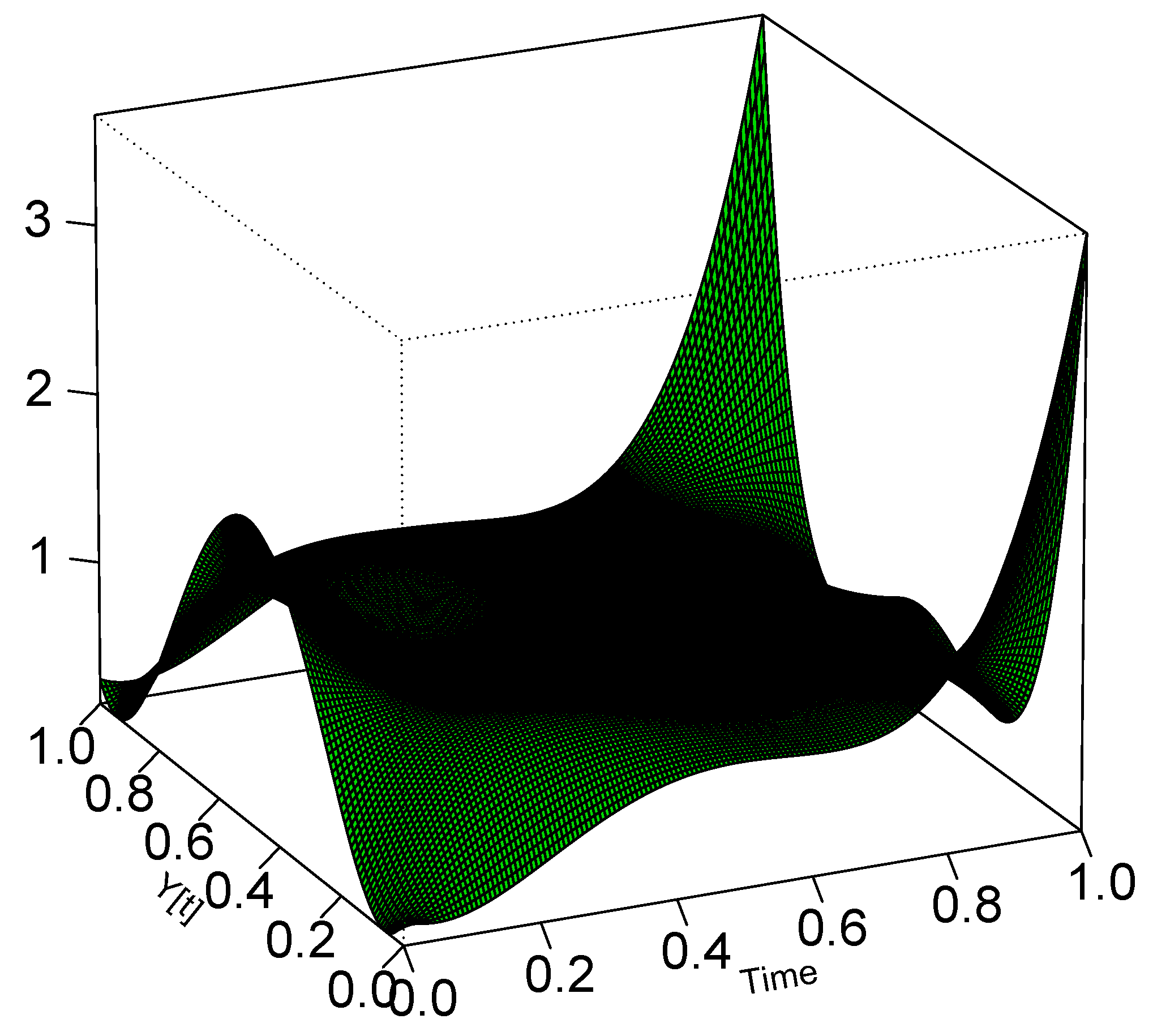
3.3.1. Nonparametric Serial Copula

We display the nonparametrically-estimated smooth serial copula density $\mathrm{cop}(u,v;Y(t),Y(t+h\left)\right)$ to get a much finer understanding of the lagged interdependence structure of a stationary time series. For a continuous distribution, define the copula density for the pair $\left(Y\right(t),Y(t+h\left)\right)$ as the joint density of $U=F\left(Y\right(t\left)\right)$ and $V=F\left(Y\right(t+h\left)\right)$, which is estimated by sample mid-distribution transform $\tilde{U}={\tilde{F}}^{\mathrm{mid}}\left(Y\left(t\right)\right)$, $\tilde{V}={\tilde{F}}^{\mathrm{mid}}\left(Y(t+h)\right)$. Following Mukhopadhyay and Parzen (2014) and Parzen and Mukhopadhyay (2012), we expand the copula density (square integrable) in a orthogonal series of product LP-basis functions as:

$$\mathrm{cop}(u,v;Y\left(t\right),Y(t+h))-1=\sum _{j,k}\mathrm{LP}[j,k;Y\left(t\right),Y(t+h)]S_j(u;Y\left(t\right))S_k(v;Y(t+h)),$$

(10)

where $S_j(u;Y\left(t\right))={\mathrm{YS}}_j(Q(u;Y\left(t\right));Y\left(t\right))$. Equation (10) allows us to pictorially represent the information present in the LP-comoment matrix via copula density. The various “shapes” of the copula density give insight into the structure and dynamics of the time series.

Now, we apply this nonparametric copula estimation theory to model the temporal dependence structure of S&P return data. The copula density estimate $\widehat{\mathrm{Cop}}(u,v;Y\left(t\right),Y(t+1))$ based on the smooth LP-comoments is displayed in Figure 3. The shape of the copula density shows strong evidence of asymmetric tail dependence. Note that the dependence is only present in the extreme quantiles, another well-known stylized fact of economic and financial time series.

3.3.2. LP-Comoment of Lag h

Here, we will introduce the concept of the LP-comoment to get a complete understanding of the nature of the serial dependence present in the data. The LP-comoment of lag h is defined as the joint covariance of $\mathrm{Vec}\left(\mathrm{YS}\right)\left(t\right)$ and $\mathrm{Vec}\left(\mathrm{YS}\right)(t+h)$.

The lag one LP-comoment matrix for S&P 500 return data is displayed below:

$$\mathrm{LP}\left[Y\left(t\right),Y(t+1)\right]=\left[\begin{array}{cccc}{0.0705}^{\ast }& -{0.0617}^{\ast }& 0.0199& 0.0113\\ 0.0074& {0.1542}^{\ast }& 0.0077& {0.0652}^{\ast }\\ -0.0104& -0.0071& 0.0262& -0.0355\\ 0.0166& {0.0438}^{\ast }& 0.0113& {0.0698}^{\ast }\end{array}\right]$$

(11)

To identify the significant elements, we first rank order the squared LP-comoments. Then, we take the penalized cumulative sum of m comoments using BIC criterion $2m\log \left(n\right)/n$, where n is the sample size, and choose the m for which the BIC is maximum. The complete BIC path for S&P 500 data is shown in Figure 3, which selects the top six comments, also denoted by $\ast$ in the LP-comoment matrix display (Equation (11)). By making all those uninteresting “small” comoments equal to zero, we get the “smooth” LP-comoment matrix denoted by $\widehat{\mathrm{LP}}$. The linear auto-correlation is captured by the $\mathrm{LP}[1,1;Y\left(t\right),Y(t+1)]=\mathbb{E}\left[{\mathrm{YS}}_1\left(t\right){\mathrm{YS}}_1(t+1)\right]$ term. The presence of higher order significant terms in the LP-comoment matrix indicates the possible nonlinearity. Another interesting point to note is that $\mathrm{CORR}\left[Y\right(t),Y(t+1\left)\right]=0.027$, whereas the auto-correlation between the mid-rank transformed data $\mathrm{CORR}[F^{\mathrm{mid}}\left(Y\left(t\right)\right),F^{\mathrm{mid}}\left(Y(t+1)\right)]=0.071$, considerably larger and picked by the BIC criterion. This is an interesting fact as it indicates that the rank-transform time series (${\mathrm{YS}}_1\left(t\right)$) is much more predictable than the original raw time series $Y\left(t\right)$.

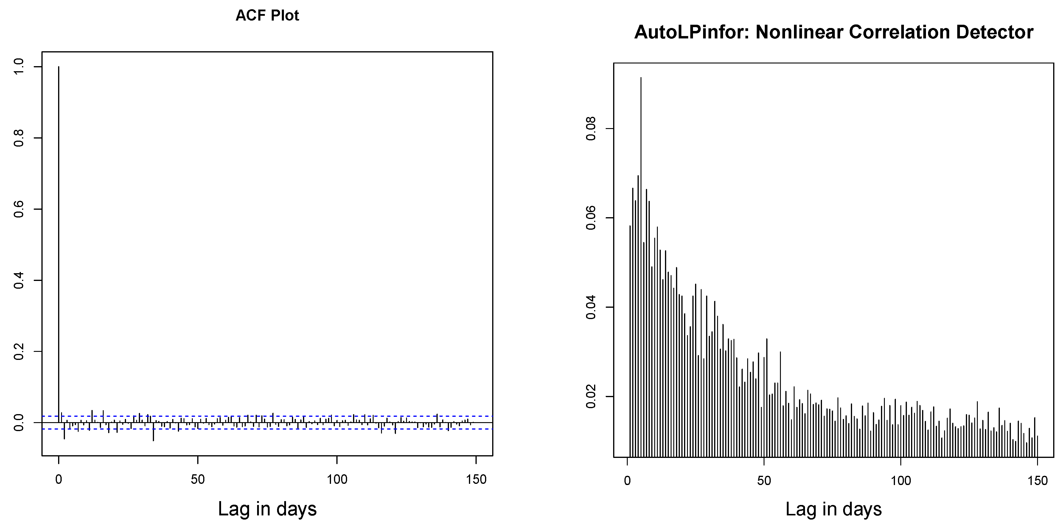
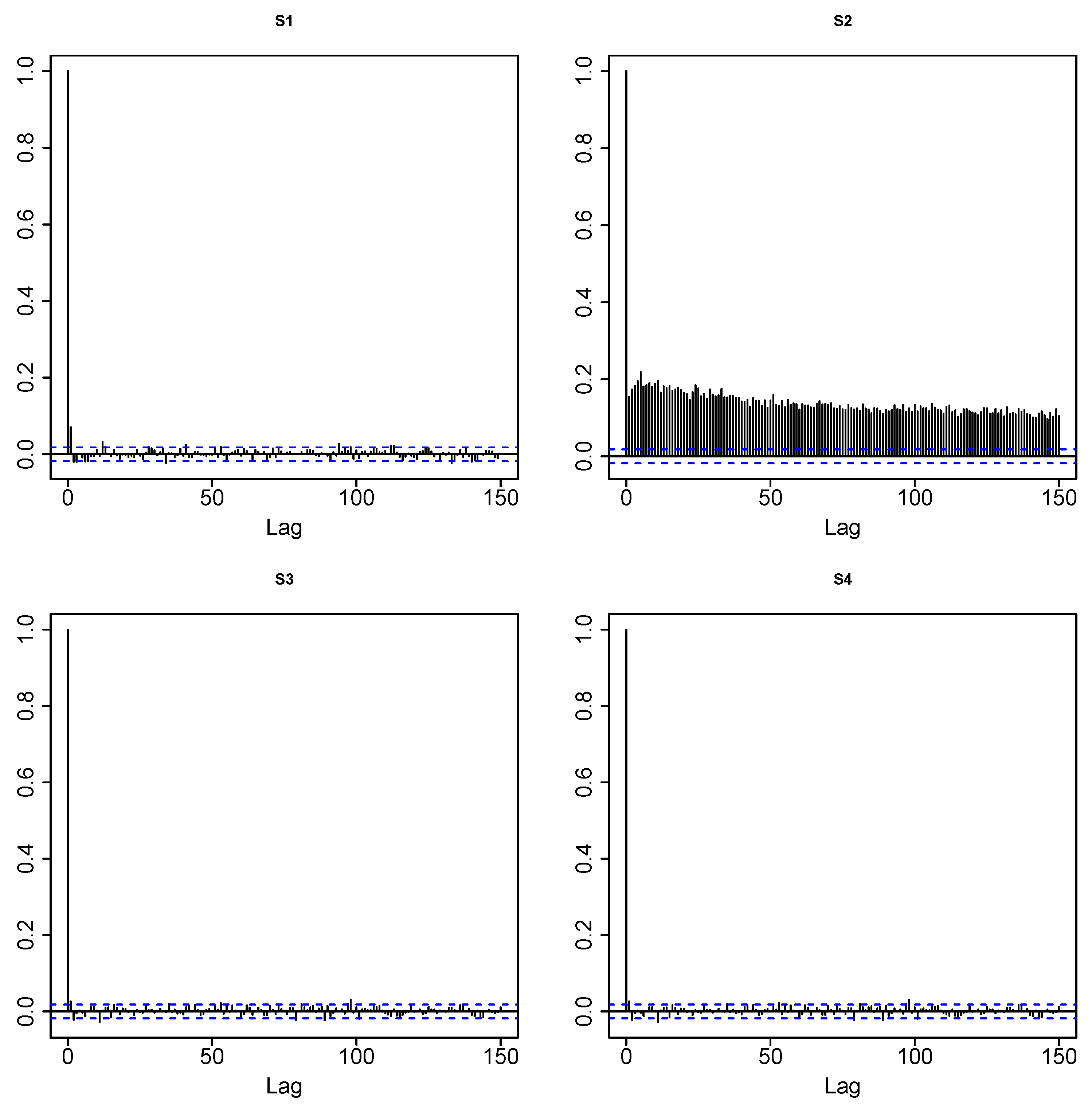
3.3.3. LP-Correlogram, Evidence and Source of Nonlinearity

We provide a nonparametric exploratory test for (non)linearity (the spectral domain test is given in Section 3.6). Plot the correlogram of ${\mathrm{YS}}_1\left(t\right),\dots ,{\mathrm{YS}}_4\left(t\right)$: (a) diagnose possible nonlinearity; and (b) identify possible sources. This constitutes an important building block for methods of model identification. The LP-correlogram generalizes the classical sample Autocorrelation Function (ACF). Applying the acf() R function on $\mathrm{Vec}\left(\mathrm{YS}\right)\left(t\right)$ generates the graphical display of our proposed LP-correlogram plot.

Figure 4 shows the LP-correlogram of S&P stock return data. Panel A shows the absence of linear autocorrelation, which is known as an efficient market hypothesis in finance literature. A prominent auto-correlation pattern for the series ${\mathrm{YS}}_2\left(t\right)$ (top right panel of Figure 4) is the source of nonlinearity. This fact is known as “volatility clustering”, which says that a large price fluctuation is more likely to be followed by large price fluctuations. Furthermore, the slow decay of the autocorrelation of the series ${\mathrm{YS}}_2\left(t\right)$ can be interpreted as an indication of the long-memory volatility structure.

3.3.4. AutoLPinfor: Nonlinear Correlation Measure

We display the sample AutoLPinforplot, a diagnostic tool for nonlinear autocorrelation. We define the lag h AutoLPinfor as the squared Frobenius norm of the smooth-LP-comoment matrix of lag h,

$$\mathrm{AutoLPinfor}\left(h\right)=\sum _{j,k}|\mathrm{LP}[j,k;Y\left(t\right),Y(t+h)]{|}^2,$$

(12)

where the sum is over BIC selected $j,k$ for which LP-comoments are significantly non-zero.

Our robust nonparametric measure can be viewed as capturing the deviation of the copula density from uniformity:

$$\begin{array}{c}\hfill \mathrm{AutoLPinfor}\left(h\right)=\int \int {\mathrm{cop}}^2[u,v;Y\left(t\right),Y(t+h)]\mathrm{d}u\mathrm{d}v-1,\end{array}$$

(13)

which is closely related to the entropy measure of association proposed in Granger and Lin (1994):

$$\begin{array}{c}\hfill \mathrm{Granger}-\mathrm{Lin}(h)=\int \int \mathrm{cop}[u,v;Y(t),Y(t+h)]\log \mathrm{cop}[u,v;Y(t),Y(t+h)]\mathrm{d}u\mathrm{d}v.\end{array}$$

(14)

It can be shown using Taylor series expansion that asymptotically:

$$\mathrm{AutoLPinfor}\left(h\right)\approx 2\times \mathrm{Granger}-\mathrm{Lin}\left(h\right).$$

(15)

An excellent discussion of the role of information theory methods for unified time series analysis is given in Parzen (1992) and Brillinger (2004). For an extensive survey of tests of independence for nonlinear processes, see Chapter 7.7 of Terasvirta et al. (2010). AutoLPinfor is a new information theoretic nonlinear autocorrelation measure, which detects generic association and serial dependence present in a time series. Contrast the AutoLPinfor plot for S&P 500 return data shown in Figure 5 with the ACF plot (left panel). This underlies the need for building a nonlinear time series model, which we will be discussing next.

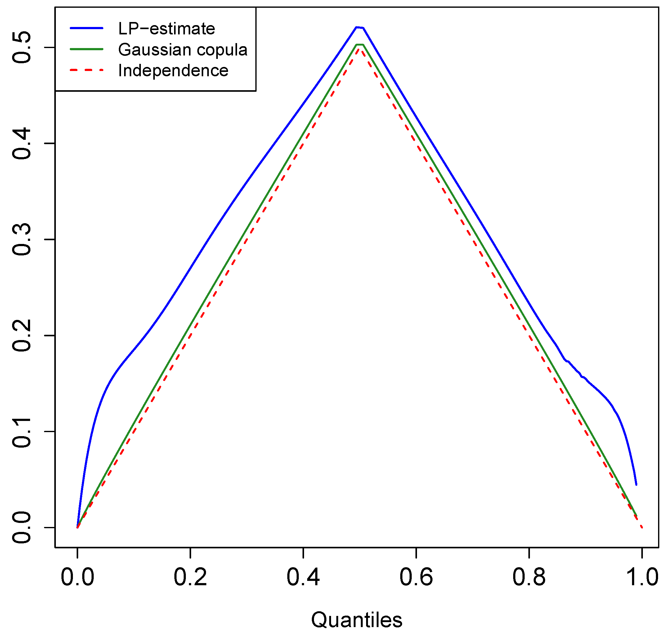
3.3.5. Nonparametric Estimation of Blomqvist’s Beta

Estimate the Blomqvist’s $\beta$ (also known as the medial correlation coefficient) of lag h by using the LP-copula estimate in the following equation,

$${\widehat{\beta }}_{\mathrm{LP}}(h;Y\left(t\right)):=-1+4{\int }_0^{1/2}{\int }_0^{1/2}\widehat{\mathrm{cop}}\left[u,v;Y\left(t\right),Y(t+h)\right]\mathrm{d}u\mathrm{d}v$$

(16)

The $\beta$ values $-1,0$ and 1 are interpreted as reverse correlation, independence and perfect correlation, respectively. Note that,

$$\begin{array}{cc}\hfill \mathrm{Blomqvist}’s\beta & :\mathrm{Normalized}\mathrm{distance}\mathrm{of}\mathrm{copula}\mathrm{distribution}\mathrm{Cop}(u,v)\mathrm{from}\mathrm{independence}\mathrm{copula}uv\hfill \\ \hfill \mathrm{AutoLPinfor}& :\mathrm{Distance}\mathrm{of}\mathrm{copula}\mathrm{density}\mathrm{Cop}(u,v)\mathrm{from}\mathrm{uniformity}1.\hfill \end{array}$$

For S&P 500 return data, we compute the following dependence numbers,

$$\begin{array}{c}{\widehat{\beta }}_{\mathrm{LP}}(1;Y\left(t\right))=0.0528\hfill \\ {\widehat{\beta }}_{\mathrm{LP}}(1;{\mathrm{YS}}_1\left(t\right))=0.0528\hfill \\ {\widehat{\beta }}_{\mathrm{LP}}(1;{\mathrm{YS}}_2\left(t\right))=0.0729\hfill \\ {\widehat{\beta }}_{\mathrm{LP}}(1;{\mathrm{YS}}_3\left(t\right))=0.0\hfill \\ {\widehat{\beta }}_{\mathrm{LP}}(1;{\mathrm{YS}}_4\left(t\right))=0.003.\hfill \end{array}$$

3.3.6. Nonstationarity Diagnosis, LP-Comoment Approach

Viewing the time index $T=1,\dots ,n$ as the covariate, we propose a nonstationarity diagnosis based on LP-comoments of $Y\left(t\right)$ and the time index variable T. Our treatment has the ability to detect the time-varying nature of mean, variance, skewness, and so on, represented by various custom-made LP-transformed time series.

For S&P data, we computed the following LP-comoment matrix to investigate the nonstationarity:

$$\mathrm{LP}\left[T,Y\left(t\right)\right]=\left[\begin{array}{cccc}0.012& {0.180}^{\ast }& -0.010& {0.058}^{\ast }\\ -0.005& -0.034& -0.036& {0.080}^{\ast }\\ -0.016& {0.115}^{\ast }& 0.001& -0.001\\ 0.024& -0.040& -0.010& {0.049}^{\ast }\end{array}\right]$$

(17)

This indicates the presence of the slight non-stationarity behavior of variance or volatility (${\mathrm{YS}}_2\left(t\right)$) and the kurtosis of tail-thickness (${\mathrm{YS}}_4\left(t\right)$). Similar to AutoLPinfor, we propose the following statistic for detecting nonstationarity:

$$\mathrm{LPinfor}[Y\left(t\right),T]=\sum _{j,k}|\mathrm{LP}[j,k;T,Y\left(t\right)]{|}^2.$$

(18)

We can also generate the corresponding smooth copula density of $(T,Y(t\left)\right)$ based on the smooth $\mathrm{LP}\left[T,Y\left(t\right)\right]$ matrix to visualize the time-varying information as in Figure 6.

3.4. Local Dependence Modeling

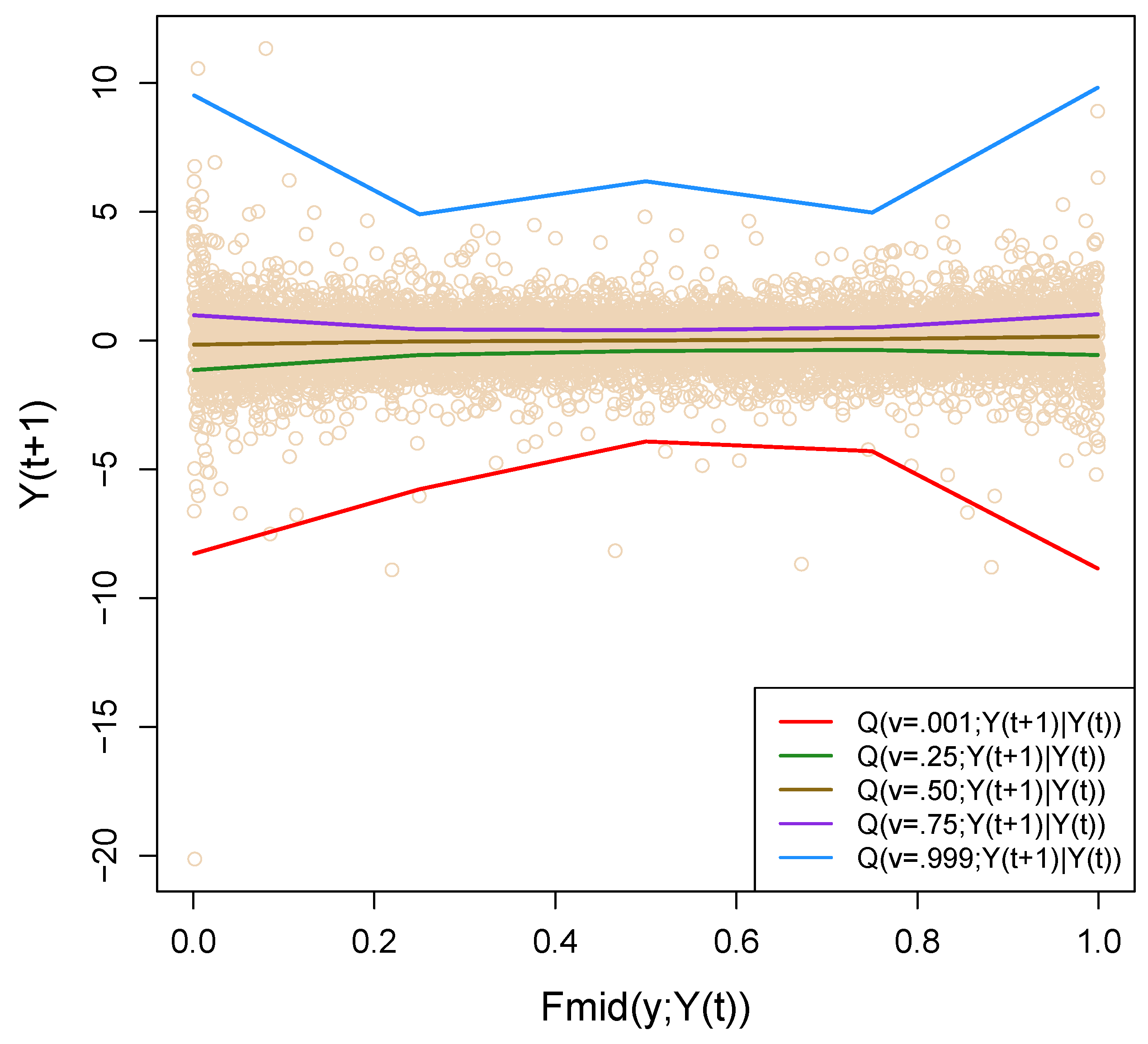
3.4.1. Quantile Correlation Plot and Test for Asymmetry

We display the quantile correlation plot, a copula distribution-based graphical diagnostic to visually examine the asymmetry of dependence. The goal is to get more insight into the nature of tail-correlation.

Motivated by the concept of the lower and upper tail dependence coefficient, we define the quantile correlation function (QCF) as the following in terms of the copula distribution function of $\left(Y\right(t),Y(t+h\left)\right)$ denoted by $\mathrm{Cop}(u,v;Y(t),Y(t+h\left)\right):=\mathrm{Cop}(u,v;h)$,

$$\lambda \left[u;Y\left(t\right),Y(t+h)\right]:={\displaystyle \frac{\mathrm{Cop}(u,u;h)}{u}}{\mathbb{I}}_{\left\{u\le 0.5\right\}}+{\displaystyle \frac{1-2u+\mathrm{Cop}(u,u;h)}{1-u}}{\mathbb{I}}_{\left\{u>0.5\right\}},$$

(19)

Our nonparametric estimate of the quantile correlation function is based on the LP-copula density, which we denote as ${\widehat{\lambda }}_{\mathrm{LP}}\left[u;Y\left(t\right),Y(t+h)\right]$. Figure 7 shows the corresponding quantile correlation plot for S&P 500 data. The dotted line represents QCF under the independence assumption. Deviation from this line helps us to better understand the nature of asymmetry. We compute ${\widehat{\lambda }}_{\mathrm{G}}[u;Y\left(t\right),Y(t+h)]$ using the fitted Gaussian copula:

$${\widehat{\mathrm{Cop}}}_{\mathrm{G}}(u,v;Y\left(t\right),Y(t+h))=\Phi ({\Phi }^{-1}\left(u\right),{\Phi }^{-1}\left(v\right);\widehat{\Sigma }=S)$$

(20)

where S is the sample covariance matrix. The dark green line in Figure 7 shows the corresponding curve, which is almost identical to the “no dependence” curve, albeit misleading. The reason is the Gaussian copula is characterized by linear correlation, while S&P data are highly nonlinear in nature. As the linear auto-correlation of a stock return is almost zero, we have approximately $\Phi ({\Phi }^{-1}\left(u\right),{\Phi }^{-1}\left(u\right);\widehat{\Sigma }=S)\approx \Phi \left({\Phi }^{-1}\left(u\right)\right)\Phi \left({\Phi }^{-1}\left(u\right)\right)=u^2$. Similar to the Gaussian copula, there are several other parametric copula families, which can give similar misleading conclusions. This simple illustration reminds us of the pernicious effect of not “looking into the data”.

3.4.2. Conditional LPinfor Dependence Measure

For more transparent and clear insight into the asymmetric nature of the tail dependence, we need to introduce the concept of conditional dependence. In what follows, we propose a conditional LPinfor function $\mathrm{LPinfor}\left(Y\right(t+h\left)\right|Y\left(t\right)=Q(u;Y(t\left)\right))$, a quantile-based diagnostic for tracking how the dependence of $Y(t+h)$ on $Y\left(t\right)$ changes at various quantiles.

To quantify the conditional dependence, we seek to estimate $f(y;Y(t+h\left)\right|Y\left(t\right))/f(y;Y(t+h))$. A brute force approach estimates separately the conditional distribution and the unconditional distribution and takes the ratio to estimate this arbitrary function. An alternative elegant way is to recognize that by “going to the quantile domain” (i.e., $Y(t+h)=Q(v;Y(t+v\left)\right)$ and $Y\left(t\right)=Q(u;Y(t\left)\right)$), we can interpret the ratio as “slices” of the copula density, which we call the conditional comparison density:

$$d\left[v;Y(t+h),Y(t+h)\left|Y\right(t)=Q(u;Y\left(t\right))\right]=1+\sum _j\mathrm{LP}[j;h,u]S_j(v;Y(t+h)),$$

(21)

where the LP-Fourier orthogonal coefficients $\mathrm{LP}[j;h]$ are given by:

$$\mathrm{LP}[j;h,u]=\sum _k\mathrm{LP}[j,k;Y\left(t\right),Y(t+h)]S_k(u;Y\left(t\right)).$$

Define the conditional LPinfor as:

$$\mathrm{LPinfor}\left[Y(t+h)\left|Y\right(t)=Q(u;Y\left(t\right))\right]=\sum _j|\mathrm{LP}[j;h,u]{|}^2.$$

(22)

We use this theory to investigate the conditional dependency structure of S&P 500 return data. Figure 8a traces out the complete path of the estimated $\mathrm{LPinfor}\left[Y\right(t+h)\mid Y(t)=Q(u;Y\left(t\right)]$ function, which indicates the high asymmetric tail correlation. These conditional correlation curves can be viewed as a “local” dependence measure. An excellent discussion on this topic is given in Section 3.3.8 of Terasvirta et al. (2010).

At this point, we can legitimately ask: What aspects of the conditional distributions are changing most? Figure 8b,c displays only the two coefficients $\mathrm{LP}[1;h,u]$ and $\mathrm{LP}[2;h,u]$ for the S&P 500 return data for the pairs $\left(Y\right(t),Y(t+1\left)\right)$. These two coefficients represent how the mean and the volatility levels of the conditional density change with respect to the unconditional reference distribution. The typical asymmetric shape of conditional volatility shown in the right panel of Figure 8b,c indicates what is known as the “leverage effect”; future stock volatility negatively correlated with past stock return, i.e., stock volatility tends to increase when stock prices drop.

3.5. Non-Crossing Conditional Quantile Modeling

We display the nonparametrically-estimated conditional quantile curves of $Y(t+h)$ given $Y\left(t\right)$. Our new modeling approach uses the estimated conditional comparison density $\widehat{d}(v;h,u)$ to simulate from $F[y;Y(t+h\left)\right|Y\left(t\right)=Q(u;Y(t\left)\right)]$ by utilizing the given sample $\tilde{Q}(u;Y\left(t\right))$ via an accept-reject rule to arrive at the “smooth” nonparametric model for $\widehat{Q}[v;Y(t+h)|Y\left(t\right)=Q(u;Y\left(t\right)]$. See Parzen and Mukhopadhyay (2013b) for details about the method. Our proposed algorithm generates “large” additional simulated samples from the conditional distribution, which allows us to accurately estimate the conditional quantiles (especially the extreme quantiles). By construction, our method is guaranteed to produce non-crossing quantile curves; thus tackling a challenging practical problem.

For S&P 500 data, we first nonparametrically estimate the conditional comparison densities $\widehat{d}(v;h,u)$ shown in the left panel of Figure 9 for $F(y;Y(t\left)\right)=0.01,0.5$ and $0.99$, which can be thought of as a “weighting function” for an unconditional marginal distribution to produce the conditional distributions:

$$\widehat{f}\left[y;Y(t+h)\left|Y\right(t)=Q(u;Y\left(t\right))\right]=f(y;Y\left(t\right))\times \widehat{d}\left[F(y;Y(t+h\left)\right);h,u\right].$$

(23)

This density estimation technique belongs to the skew-G modeling class (Mukhopadhyay 2016). We simulate n = 10,000 samples from $\widehat{f}(y;Y(t+h)|Y\left(t\right))$ by accept-reject sampling from $\widehat{d}(v;h,u)$, $u=\{0.01,0.5,0.99\}$. The histograms and the smooth conditional densities are shown in the right panel of Figure 9. It shows some typical shapes in terms of long-tailedness.

Next, we proceed to estimate the nonparametric conditional quantiles $\widehat{Q}(v;Y(t+h)|Y\left(t\right))$, for $v=0.001,0.25,0.5,0.75,0.999$, from the simulated data. Figure 10 shows the estimated conditional quantiles. The extreme conditional quantiles have a special significance in the context of financial time series. They are sometimes popularly known as Conditional Value at Risk (CoVaR), currently the most popular quantitative risk management tool (see Adrian and Brunnermeier (2011); Engle and Manganelli (2004)). The red solid line in Figure 10 is $\widehat{Q}\left[0.001;Y(t+1)\mid Y\left(t\right)=Q(u;Y(t\left)\right)\right]$, which is known as the 0.1% CoVaR function for a one-day holding period for S&P 500 daily return data. Although the upper conditional quantile curve $\widehat{Q}(0.999;Y(t+1)|Y\left(t\right))$ (blue solid line) shows symmetric behavior around $F(y;Y(t\left)\right)=0.5$, the lower quantile has a prominent asymmetric shape. These conditional quantiles give the ultimate description of the auto-regressive dependence of S&P 500 return movement in the tail region.

3.6. Nonlinear Spectrum Analysis

Here, we extend the concept of spectral density for nonlinear processes. We display the LPSpectrum -Autoregressive (AR) spectral density estimates of ${\mathrm{YS}}_1\left(t\right),\dots ,{\mathrm{YS}}_4\left(t\right)$. The spectral density for each LP-transformed series is defined as:

$$\begin{array}{ccc}\hfill f(\omega ;{\mathrm{YS}}_j)& =& \sum _h\mathrm{LP}[j,j;Y\left(t\right),Y(t+h)]e^{-i2\pi h\omega },-1/2<\omega <1/2\hfill \\ & =& \sum _h\mathrm{Cov}[{\mathrm{YS}}_j\left(t\right),{\mathrm{YS}}_j(t+h)]e^{-i2\pi h\omega },-1/2<\omega <1/2.\hfill \end{array}$$

(24)

We separately fit the univariate AR model for the components of $\mathrm{Vec}\left(\mathrm{YS}\right)\left(t\right)$ and use the BIC order selection criterion to select the “best” parsimonious parametrization using the Burg method.

Finally, we use the estimated model coefficients to produce the “smooth” estimate of the spectral density function (see Equation (2)). The copula spectral density is defined as:

$$f(\omega ;u,v)=\sum _h\mathrm{Cop}(u,v;h)e^{-i2\pi h\omega },-1/2<\omega <1/2.$$

(25)

To estimate the copula spectral density, we use the LP-comoment-based nonparametric copula density estimate. Note that both the serial copula (3.12) and the corresponding spectral density (3.25) capture the same amount of information for the serial dependence of $\left\{Y\right(t\left)\right\}$. For that reason, we recommend computing AutoLPinfor as a general dependence measure for non-Gaussian nonlinear processes.

The application of our LPSpectral tool on S&P 500 return data is shown in Figure 11. A few interesting observations are: (i) the conventional spectral density (black solid line) provides no insight into the (complex) serial dependency present in the data; (ii) the nonlinearity in the series is captured by the interesting shapes of our specially-designed times series ${\mathrm{YS}}_2\left(t\right)$ and ${\mathrm{YS}}_4\left(t\right)$, which classical (linear) correlogram-based spectra cannot account for; (iii) the shape of the spectra of $\mathcal{Z}\left(Y\right(t\left)\right)$ and the rank-transformed time series ${\mathrm{YS}}_1\left(t\right)$ look very similar; and a (iv) pronounced singularity near zero of the spectrum of ${\mathrm{YS}}_2\left(t\right)$ hints at some kind of “long-memory” behavior. This phenomena is also known as regular variation representation at frequency $\omega =0$ (Granger and Joyeux 1980).

A quick diagnostic measure for screening significant spectrums can be computed via the information number $2{\int }_0^{1/2}\log \widehat{f}(\omega ;S_j)\mathrm{d}\omega$. The LPSpectrum methodology is highly robust and, thus, can tackle the heavy-tailed S&P data quite successfully.

3.7. Nonparametric Model Specification

The ultimate goal of empirical time series analysis is nonparametric model identification. To model the univariate stationary nonlinear process, we specify the multiple autoregressive model based on $\mathrm{Vec}\left(\mathrm{YS}\right)\left(t\right)={\left[{\mathrm{YS}}_1\left(t\right),\dots ,{\mathrm{YS}}_k\left(t\right)\right]}^T$ of the form:

$$\mathrm{Vec}\left(\mathrm{YS}\right)\left(t\right)=\sum _{k=1}^{m}A(k;m)\mathrm{Vec}\left(\mathrm{YS}\right)(t-k)+\mathit{ϵ}\left(t\right).$$

(26)

where $\mathit{ϵ}\left(t\right)$ is multivariate mean zero Gaussian white noise with covariance ${\Sigma }_m$. This system of equations jointly describes the dynamics of the nonlinear process and how it evolves over time. We use the BIC criterion to select the model order m, which minimizes:

$$\mathrm{BIC}\left(m\right)=\log |{\widehat{\Sigma }}_m|+m{k}^2{\displaystyle \frac{\log T}{T}}.$$

(27)

We carry out this step for our S&P 500 return data. We estimate our multiple AR model based on $\mathrm{Vec}\left(\mathrm{YS}\right)\left(t\right)={\left[{\mathrm{YS}}_1\left(t\right),{\mathrm{YS}}_2\left(t\right),{\mathrm{YS}}_4\left(t\right)\right]}^T$. We discard ${\mathrm{YS}}_3\left(t\right)$ due to its flat spectrum (see Figure 11). BIC selects “best” order eight. Although the complete description of the estimated model is clearly cumbersome, we provide below the approximate structure by selecting a few large coefficients from the actual matrix equation. The goal is to interpret the coefficients (statistical parameters) of the estimated model and relate them to economic theory (scientific parameters/theory). This multiple AR LP-model (LPVAR) is given by:

$$\begin{array}{ccc}{\mathrm{YS}}_1\left(t\right)\hfill & \approx \hfill & 0.071{\mathrm{YS}}_1(t-1)-0.024{\mathrm{YS}}_1(t-2)+{ϵ}_1\left(t\right)\hfill \\ {\mathrm{YS}}_2\left(t\right)\hfill & \approx \hfill & -0.063{\mathrm{YS}}_1(t-1)-0.075{\mathrm{YS}}_1(t-2)+0.06{\mathrm{YS}}_2(t-2)+0.123{\mathrm{YS}}_2(t-5)+0.04{\mathrm{YS}}_4(t-2)+{ϵ}_2\left(t\right)\hfill \\ {\mathrm{YS}}_4\left(t\right)\hfill & \approx \hfill & 0.04{\mathrm{YS}}_4(t-1)+0.038{\mathrm{YS}}_4(t-2)+0.04{\mathrm{YS}}_2(t-3)+{ϵ}_4\left(t\right).\hfill \end{array}$$

(28)

and the residual covariance matrix is:

$$\widehat{{\Sigma }_8}=\left[\begin{array}{ccc}0.993& -0.001& -0.002\\ -0.001& 0.853& -0.058\\ -0.002& -0.058& 0.964\end{array}\right]$$

The autoregressive model of ${\mathrm{YS}}_2\left(t\right)$ can be considered as a robust stock return volatility model (LPVolatility modeling), which is less affected by unusually large extreme events. The model for ${\mathrm{YS}}_2\left(t\right)$ automatically discovers many known facts: (a) the sign of the coefficient linking volatility and return is negative, confirming the “leverage effect”; (b) ${\mathrm{YS}}_2\left(t\right)$ is positively autocorrelated, known as volatility clustering; (c) the positive interaction with lagged ${\mathrm{YS}}_4\left(t\right)$ accounts for the “excess kurtosis”.

4. Conclusions

This article provides a pragmatic and comprehensive framework for nonlinear time series modeling that is easier to use, more versatile and has a strong theoretical foundation based on the recently-developed theory of unified algorithms of data science via LP modeling (Mukhopadhyay 2016, 2017; Mukhopadhyay and Fletcher 2018; Mukhopadhyay and Parzen 2014; Parzen and Mukhopadhyay 2012, 2013a, 2013b). The summary and broader implications of the proposed research are:

• From the theoretical standpoint, the unique aspect of our proposal lies in its ability to simultaneously embrace and employ the spectral domain, time domain, quantile domain and information domain analyses for enhanced insights, which to the best of our knowledge has not appeared in the nonlinear time series literature before.
• From a practical angle, the novelty of our technique is that it permits us to use the techniques from linear Gaussian time series to create non-Gaussian nonlinear time series models with highly interpretable parameters. This aspect makes LPTime computationally extremely attractive for data scientists, as they can now borrow all the standard time series analysis machinery from R libraries for implementation purposes.
• From the pedagogical side, we believe that these concepts and methods can easily be augmented with the standard time series analysis course to modernize the current curriculum so that students can handle complex time series modeling problems (McNeil et al. 2010) using the tools with which they are already familiar.

The main thrust of this article is to describe and interpret the steps of LPTime technology to create a realistic general-purpose algorithm for empirical time series modeling. In addition, many new theoretical results and diagnostic measures were presented, which laid the foundation for the algorithmic implementation of LPTime. We showed how LPTime can systematically explore the data to discover empirical facts hidden in time series. For example, LPTime empirical modeling of S&P 500 return data reproduces the ‘stylized facts’—(a) heavy tails; (b) non-Gaussian; (c) nonlinear serial dependence; (d) tail correlation; (e) asymmetric dependence; (f) volatility clustering; (g) long-memory volatility structure; (h) efficient market hypothesis; (i) leverage effect; (j) excess kurtosis—in a coherent manner under a single general unified framework. We have emphasized how the statistical parameters of our model can be interpreted in light of established economic theory.

We have recently applied this theory for large-scale eye-movement pattern discovery problem, which came out as the winner (among 82 competing algorithms) of the 2014 IEEE International Biometric Eye Movements Verification and Identification Competition (Mukhopadhyay and Nandi 2017). The proposed algorithm is implemented in the R package LPTime (Mukhopadhyay and Nandi 2015), which is available on CRAN.

We conclude with some general references: a few popular articles: Brillinger (1977, 2004); Engle (1982); Granger and Lin (1994); Granger (1993, 2003); Parzen (1967, 1979); Salmon (2012); Tukey (1980); books: Guo et al. (2017); Terasvirta et al. (2010); Tsay (2010); Woodward et al. (2011); and review articles: Granger (1998); Hendry (2011).

References

1. Adrian, Tobias, and Markus K Brunnermeier. 2011. Covar. Technical Report. Cambridge: National Bureau of Economic Research. [Google Scholar]
2. Brillinger, David R. 1977. The identification of a particular nonlinear time series system. Biometrika 64: 509–15. [Google Scholar] [CrossRef]
3. Brillinger, David R. 2004. Some data analyses using mutual information. Brazilian Journal of Probability and Statistics 18: 163–83. [Google Scholar]
4. Engle, Robert F. 1982. Autoregressive conditional heteroscedasticity with estimates of the variance of united kingdom inflation. Econometrica: Journal of the Econometric Society 50: 987–1007. [Google Scholar] [CrossRef]
5. Engle, Robert F., and Simone Manganelli. 2004. Caviar: Conditional autoregressive value at risk by regression quantiles. Journal of Business & Economic Statistics 22: 367–81. [Google Scholar]
6. Granger, Clive, and Jin-Lung Lin. 1994. Using the mutual information coefficient to identify lags in nonlinear models. Journal of Time Series Analysis 15: 371–84. [Google Scholar] [CrossRef]
7. Granger, Clive W. J. 1993. Strategies for modelling nonlinear time-series relationships. Economic Record 69: 233–38. [Google Scholar] [CrossRef]
8. Granger, Clive W. J. 1998. Overview of nonlinear time series specification in economics. Paper presented at the NSF Symposium on Nonlinear Time Series Models, University of California, Berkeley, CA, USA, 22 May 1998. [Google Scholar]
9. Granger, Clive W. J. 2003. Time series concepts for conditional distributions. Oxford Bulletin of Economics and Statistics 65: 689–701. [Google Scholar] [CrossRef]
10. Granger, Clive W. J., and Roselyne Joyeux. 1980. An introduction to long-memory time series models and fractional differencing. Journal of Time Series Analysis 1: 15–29. [Google Scholar] [CrossRef]
11. Guo, Xin, Howard Shek, Tze Leung Lai, and Samuel Po-Shing Wong. 2017. Quantitative Trading: Algorithms, Analytics, Data, Models, Optimization. New York: Chapman and Hall/CRC. [Google Scholar]
12. Hendry, David F. 2011. Empirical economic model discovery and theory evaluation. Rationality, Markets and Morals 2: 115–45. [Google Scholar]
13. McNeil, Alexander J., Rüdiger Frey, and Paul Embrechts. 2010. Quantitative Risk Management: Concepts, Techniques, and Tools. Princeton: Princeton University Press. [Google Scholar]
14. Mukhopadhyay, Subhadeep. 2016. Large scale signal detection: A unifying view. Biometrics 72: 325–34. [Google Scholar] [CrossRef] [PubMed]
15. Mukhopadhyay, Subhadeep. 2017. Large-scale mode identification and data-driven sciences. Electronic Journal of Statistics 11: 215–40. [Google Scholar] [CrossRef]
16. Mukhopadhyay, Subhadeep, and Douglas Fletcher. 2018. Generalized Empirical Bayes Modeling via Frequentist Goodness-of-Fit. Nature Scientific Reports 8: 1–15. [Google Scholar] [CrossRef] [PubMed]
17. Mukhopadhyay, Subhadeep, and Shinjini Nandi. 2015. LPTime: LP Nonparametric Approach to Non-Gaussian Non-Linear Time Series Modelling. CRAN, R Package Version 1.0-2. Ithaca: Cornell University Library. [Google Scholar]
18. Mukhopadhyay, Subhadeep, and Shinjini Nandi. 2017. LPiTrack: Eye movement pattern recognition algorithm and application to biometric identification. Machine Learning. [Google Scholar] [CrossRef]
19. Mukhopadhyay, Subhadeep, and Emanuel Parzen. 2014. LP approach to statistical modeling. arXiv, arXiv:1405.2601. [Google Scholar]
20. Parzen, Emanuel. 1967. On empirical multiple time series analysis. In Statistics, Proceedings of the Fifth Berkeley Symposium on Mathematical Statistics and Probability. Berkeley: University of California Press, vol. 1, pp. 305–40. [Google Scholar]
21. Parzen, Emanuel. 1979. Nonparametric statistical data modeling (with discussion). Journal of the American Statistical Association 74: 105–31. [Google Scholar] [CrossRef]
22. Parzen, Emanuel. 1992. Time series, statistics, and information. In New Directions in Time Series Analysis. Edited by Emanuel Parzen, Murad Taqqu, David R. Brillinger, Peter Caines, John Geweke and Murray Rosenblatt. New York: Springer Verlag, pp. 265–86. [Google Scholar]
23. Parzen, Emanuel. 1997. Comparison distributions and quantile limit theorems. Paper presented at the International Conference on Asymptotic Methods in Probability and Statistics, Carleton University, Ottawa, ON, Canada, July 8–13. [Google Scholar]
24. Parzen, Emanuel, and Subhadeep Mukhopadhyay. 2012. Modeling, Dependence, Classification, United Statistical Science, Many Cultures. arXiv, arXiv:1204.4699. [Google Scholar]
25. Parzen, Emanuel, and Subhadeep Mukhopadhyay. 2013a. United Statistical Algorithms, LP comoment, Copula Density, Nonparametric Modeling. Paper presented at the 59th ISI World Statistics Congress (WSC) of the International Statistical Institute, Hong Kong, China, August 25–30. [Google Scholar]
26. Parzen, Emanuel, and Subhadeep Mukhopadhyay. 2013b. United Statistical Algorithms, Small and Big Data, Future of Statisticians. arXiv, arXiv:1308.0641. [Google Scholar]
27. Salmon, Felix. 2012. The formula that killed wall street. Significance 9: 16–20. [Google Scholar] [CrossRef]
28. Terasvirta, Timo, Dag Tjøstheim, and Clive W. J. Granger. 2010. Modelling Nonlinear Economic Time Series. Kettering: OUP Catalogue. [Google Scholar]
29. Tsay, Ruey S. 2010. Analysis of Financial Time Series. Hoboken: Wiley. [Google Scholar]
30. Tukey, John. 1980. Can we predict where “time series” should go next. In Directions in Times Series. Hayward: IMS, pp. 1–31. [Google Scholar]
31. Woodward, Wayne A., Henry L. Gray, and Alan C. Elliott. 2011. Applied Time Series Analysis. Boca Raton: CRC Press. [Google Scholar]
1
The LP nomenclature: In nonparametric statistics, the letter L plays a special role to denote robust methods based on ranks and order statistics such as quantile-domain methods. With the same motivation, we use the letter L. On the other hand, P simply stands for Polynomials. Our custom-constructed basis functions are orthonormal polynomials of mid-rank transform instead of raw y-values; for more details see Mukhopadhyay and Parzen (2014).
Figure 1. LP-transformed S&P 500 daily stock returns between October 1986 and October 1988. This is just a small part of the full time series from 2 January 1963–31 December 2009 (cf. Section 3.1).
Jrfm 11 00037 g001
Figure 2. (a) The marginal distribution of daily returns; (b) plots the histogram of Φ ( y i ) and display the LP-estimated comparison density curve. and (c) shows the associated comparison density estimate with G as t-distribution with 2 degrees of freedom.
Jrfm 11 00037 g002
Figure 3. Top: Nonparametric smooth serial copula density (lag one) estimate of S&P return data. Bottom: BIC plot to select the significant LP-comoments computed in Equation (11).
Jrfm 11 00037 g003
Figure 4. LP-correlogram: Sample autocorrelations of LP-transformed time series. The decay rate of the sample autocorrelations of YS 2 ( t ) appears to be much slower than the exponential decay of the ARMA process, implying possible long-memory behavior.
Jrfm 11 00037 g004
Figure 5. Left: ACF plot of S&P 500 data. Right: AutoLPinforPlot up to lag 150.
Jrfm 11 00037 g005
Figure 6. LP copula diagnostic for detecting non-stationarity in S&P 500 return data.
Jrfm 11 00037 g006
Figure 7. Estimated Quantile Correlation Function (QCF) λ ^ LP [ u ; Y ( t ) , Y ( t + 1 ) ] . It detects asymmetry in the tail dependence between the lower-left quadrant and upper-right quadrant for S&P 500 return data. The red dotted line denotes the quantile correlation function under dependence. The dark green line shows the quantile correlation curve for the fitted Gaussian copula.
Jrfm 11 00037 g007
Figure 8. (a) The conditional LPinfor curve is shown for the pair [ Y ( t ) , Y ( t + 1 ) ] . The asymmetric dependence in the tails is clearly shown, and almost nothing is going on in between. (b,c) Display of how the mean and volatility levels of conditional distribution f [ y ; Y ( t + 1 ) | Y ( t ) = Q ( u ; Y ( t ) ) ] change with respect to the unconditional marginal distribution f ( y ; Y ( t ) ) at different quantiles.
Jrfm 11 00037 g008
Figure 9. Each row displays the estimated conditional comparison density and the corresponding conditional distribution for u = 0.01 , 0.5 , 0.99 .
Jrfm 11 00037 g009
Figure 10. The figure shows estimated non-parametric conditional quantile curves for S&p 500 return data. The red solid line, which represents Q ^ ( 0.001 ; Y ( t + 1 ) | Y ( t ) ) , is popularly known as the one-day 0.1% Conditional Value at Risk measure (CoVaR).
Jrfm 11 00037 g010
Figure 11. LPSpectrum: AR spectral density estimate for S&P 500 return data. Order selected by the BIC method. This provides a diagnostic tool for providing evidence of hidden periodicities in non-Gaussian nonlinear time series.
Jrfm 11 00037 g011