Variance Swap Replication: Discrete or Continuous?

Abstract

The popular replication formula to price variance swaps assumes continuity of traded option strikes. In practice, however, there is only a discrete set of option strikes traded on the market. We present here different discrete replication strategies and explain why the continuous replication price is more relevant.

1. Introduction

Variance swaps contracts allow a buyer to receive the future realized variance of the price changes until a specific maturity date against a fixed strike price, paid at maturity. Conventionally, these price changes are daily log returns of a specific stock, equity index or exchange rate based on the most commonly-used closing price (or exchange rate reset price). Variance swaps became particularly popular after Demeterfi et al. showed that a single contract could be statically replicated by a portfolio of vanilla options Demeterfi et al. (1999). These swaps allow hedge funds to speculate on future realized volatility and banks to trade the spread between realized and implied volatility, as well as to hedge their volatility exposure of other positions.

The very popular replication given by Demeterfi et al. by a discrete set of option prices in Demeterfi et al. (1999) is only one of the possible approximations of the continuous replication formula from Carr and Madan Carr and Madan (2001). Leung and Lorig investigate static hedging more generally by a discrete set of forwards, bonds and options prices in Leung and Lorig (2016) and describe a method to find the optimal discrete quadratic hedge under a cost constraint. This paper stays in the Carr and Madan framework, but analyzes other possible simple discrete replications for the variance swap that can be better in terms of direct hedge than the solution from Leung and Lorig, which is optimal only in terms of quadratic hedging error. This paper then explains the problem of truncation and explores the effects of tail events, stochastic volatility and jumps on variance swaps and volatility swaps. It is found that the latter behave significantly differently.

In Fukasawa et al. (2011), Fukasawa et al. describe a practical continuous replication for the variance swap based on market quotes. While their technique is elegant and their interpolation methodology is sound, they do not explore the issue of discrete replication or truncation. Their idea is to propose an alternative standard methodology to the CBOE VIXindex calculation. In practice, their method produces prices very close to the one obtained by the direct implementation of the Carr–Madan continuous replication formula as described in this paper.

Jiang and Tian explain the discretization and truncation errors in the calculation of the VIX index with the CBOE methodology in Jiang and Tian (2007). The VIX index corresponds to a specific discretization of the continuous replication of a variance swap of maturity in 30 days on the SPX500 index. Although their paper properly sheds light on discretization and truncation errors, it somewhat contradicts their earlier similar paper Jiang and Tian (2005). In the more recent paper, they explain that the VIX index is not so close to the theoretical continuous variance, while in the older paper, they explain that the variance is properly captured as the market strikes are on one side dense enough to make the discretization effect negligible and on the other side available for a large enough range so that truncation is not an issue. The present paper is more concerned about the valuation of standard variance swaps, whose typical maturity is one year. Truncation and discretization play a more important role, especially on assets that are less liquid than the SPX500 index. It also focuses on discrete hedging, with a close look at Demeterfi et al.’s methodology, often considered a standard in the industry. Finally, it analyzes the behavior of the volatility swap towards truncation and jumps comparatively to the variance swap. It neglects however any bias related to the fact that the variance is typically monitored daily instead of continuously in the variance swap contract, analyzed in Broadie and Jain (2008).

In the case of the variance swap, Demeferti et al. show that the effect of jumps on the replication of the variance swap is approximately cubic in the jump size. Carr and Wu give a more general expression of the error incurred by ignoring jumps in a replication in Carr and Wu (2008) and suggest that it can be ignored in the case of the 30-day variance. In this paper, we show that the effect is not necessarily so small on one-year variance swaps and look comparatively at the effect of jumps on the volatility swap replication.

2. Variance Swap

The payoff V of a variance swap with volatility strike K and observations at dates $t_i$ at maturity T is:

$$V(K,0)=u^2\sum _{0<t_i\le T}{\left(ln\frac{S_{t_i}}{S_{t_{i-1}}}\right)}^2-K^2$$

(1)

where u is a scaling factor. Typically, for an annualization of 252, common in practice, we have $u=100\sqrt{252/N}$.

We assume, unless specifically mentioned, no cash dividend on the asset S. Proportional dividends are however acceptable if the log-returns are adjusted by the dividend value, which is usually the case for single name equities. A continuous dividend yield is also acceptable.

Let $F(t,T)$ be the forward price of the asset S at maturity T. With an interest rate r and dividend yield q, $F(t,T)=S(t)e^{{\int }_t^{T}r(\tau )-q(\tau )d\tau }$. Assuming the absence of arbitrage opportunities and no jumps, the process F is a martingale and follows:

$$\frac{dF}{F}=\sigma (t,\cdots )dW$$

(2)

where the volatility $\sigma$ is an arbitrary stochastic process. We approximate the discrete variance by the continuous variance to obtain:

$$\begin{array}{cc}\hfill V(0,T)& \approx u^2\mathbb{E}\left[\frac{1}{T}{\int }_0^T{\sigma }^2(t,\cdots )dt\right]\hfill \\ & =u^2\mathbb{E}\left[\frac{2}{T}\left({\int }_0^T\frac{dF}{F}-ln\frac{F(T,T)}{F(0,T)}\right)\right]\hfill \\ & =u^2\mathbb{E}\left[-\frac{2}{T}ln\frac{F(T,T)}{F(0,T)}\right].\hfill \end{array}$$

(3)

An application of the replication formula from Carr and Madan (2001) leads to:

$$V(K,T)=u^{2}DF(T)\left({\int }_0^{F(0,T)}\frac{2}{K^2}P(K,T)dK+{\int }_{F(0,T)}^{+\infty }\frac{2}{K^2}C(K,T)dK\right)-DF(T)K^2$$

(4)

where $C(K,T)$ and $P(K,T)$ are respectively undiscounted call and put option prices of strike K and maturity T, and $DF(T)$ is the discount factor to time T taken from the relevant discount curve.

3. Volatility Swap

The payoff of a volatility swap of strike K at maturity T is:

$$V_{\mathrm{vol}}(K,0)=u\sqrt{\sum _{0<t_i\le T}{\left(ln\frac{S_{t_i}}{S_{t_{i-1}}}\right)}^2}-K.$$

(5)

While it is very similar, the replication is not as simple, and only closed-form approximations are available, such as the one from Carr and Lee (2008). Their replication of the volatility swap initial value leads to:

$$\begin{array}{cc}\hfill V_{\mathrm{vol}}(K,T)& \approx uDF(T)\left(-{\int }_0^{F(0,T)}\sqrt{\frac{\pi }{8K^{3}F}}\left[I_1(k)-I_0(k)\right]P(K,T)dK\right.\hfill \\ & +{\int }_{F(0,T)}^{+\infty }\sqrt{\frac{\pi }{8K^{3}F}}\left[I_1(k)-I_0(k)\right]C(K,T)dK\hfill \\ & \left.+\sqrt{\frac{\pi }{2}}\frac{C(F,T)+P(F,T)}{F(0,T)}\right)-DF(T)K\hfill \end{array}$$

(6)

where $k=ln\frac{K}{F(0,T)}$ and $I_0,I_1$ are order-zero and order-one modified Bessel functions of the first kind.

The last term, which corresponds to a specific quantity of at-the-money straddle options, is the dominant term. The Carr–Lee replication payoff for the volatility swap looks like a straddle with modified wings.

4. Continuous Replication in Practice

In reality, the market is composed of a discrete set of option prices for a given maturity. In order to find the put and call prices for any strike, a volatility surface interpolation method must be used. Some typical choices are a cubic spline, typically in variance vs. log-moneyness combined with a linear extrapolation as in Jiang and Tian (2007), a parametric model such as SVI Gatheral (2004) or some arbitrage-free method such as Andreasen and Huge one-step interpolation Andreasen and Huge (2010). The integration is truncated before zero at $K_{min}$ and before $+\infty$ at $K_{max}$. The present value of the contract can then be computed by an adaptive Gauss–Lobatto quadrature Espelid (2003); Gander and Gautschi (2000). Initial values for $K_{min}$ and $K_{max}$ are computed assuming that the asset behaves like a geometrical Brownian motion process by:

$$\begin{array}{cc}\hfill K_{min}& =F(0,T)e^{{\mathsf{\Phi }}^{-1}(ϵ)\sigma \sqrt{T}},\hfill \end{array}$$

(7)

$$\begin{array}{cc}\hfill K_{max}& =F(0,T)e^{-{\mathsf{\Phi }}^{-1}(ϵ)\sigma \sqrt{T}}\hfill \end{array}$$

(8)

where ${\mathsf{\Phi }}^{-1}$ is the inverse cumulative normal function, $ϵ$ is a tolerance (for example, $ϵ={10}^{-6}$) and $\sigma$ the at-the-money implied volatility. We then refine $K_{max}$ and $K_{min}$ by integrating step by step between $(\frac{K_{min}}{n+1},\frac{K_{min}}{n})$ and $(n{K}_{max},(n+1)K_{max})$ until those integrals have a lower value than the tolerance.

The implementation benefits from a log-transformation $y=ln\frac{K}{F(0,T)}$. The replication formula then simplifies to:

$$\begin{array}{cc}\hfill V(K,T)& =\frac{u^{2}B(0,T)}{2T}\left[{\int }_{y_{min}}^0-e^{-y}\mathsf{\Phi }\left(-d_1(y)\right)+\mathsf{\Phi }\left(-d_2(y)\right)dy\right.\hfill \\ & \left.+{\int }_0^{y_{max}}{e}^{-y}\mathsf{\Phi }\left(d_1(y)\right)-\mathsf{\Phi }\left(d_2(y)\right)dy\right]-B(0,T)K^2\hfill \end{array}$$

(9)

with $d_1(y)=\frac{1}{2}\sigma (y,T)\sqrt{T}-\frac{y}{\sigma (y,T)\sqrt{T}}$, $d_2(y)=d_1(y)-\sigma (y,T)\sqrt{T}$.

The above methodology is similar to what is proposed by Jiang and Tian (2007), but we leave the choice of interpolation open and advocate an adaptive quadrature instead of a trapezoidal discretization with no clear number of steps on a fixed range.

Fukasawa et al. propose an alternative approach in Fukasawa et al. (2011). While their technique has several merits with regards to the consistency of their interpolation methodology, it leads to prices very close to the one obtained by the more direct implementation of the Carr–Madan formula described above.

5. Discrete Replication

5.1. Derman’s Method

The idea of Demeterfi et al. is to approximate the ln payoff by a piecewise-linear function, as piecewise-linear functions can be exactly replicated by a stream of call and put options Demeterfi et al. (1999). The replication formula of Carr and Madan (2001) is not directly used.

We consider a set of increasing call option strikes $K_i^c$ and a set of decreasing put option strikes $K_i^p$ for $i=0,\cdots ,n$ with $K_0^c=K_0^p=K_0$.

Because the forward $F(0,T)$ might not fall exactly on a strike, we need to slightly rewrite Equation (3).

$$\begin{array}{cc}\hfill ln\frac{F(T,T)}{F(0,T)}& =ln\frac{F(T,T)}{K_0}+ln\frac{K_0}{F(0,T)}.\hfill \end{array}$$

(10)

Instead of replicating directly $ln\frac{F(T,T)}{K_0}$, Demeterfi et al. work directly with the payoff:

$$f(x)=\frac{x}{K_0}-1-ln(\frac{x}{K_0}).$$

(11)

Note that the linear term can be omitted, as it can also directly be replicated by shares, but in the end, this would lead to the exact same price, by linearity.

Figure 1a shows the payoff and the piecewise-linear approximation.

The slope of each segment leads to call and put option weights $w^c(K_i^c),w^p(K_i^p)$:

$$\begin{array}{cc}\hfill w^c(K_0)& =\frac{f(K_1^c)-f(K_0)}{K_1^c-K_0}\hfill \end{array}$$

(12)

$$\begin{array}{cc}\hfill w^c(K_i^c)& =\frac{f(K_{i+1}^c)-f(K_i^c)}{K_{i+1}^c-K_i^c}-\sum _{j=0}^{i-1}{w}^c(K_i^c)\hfill \end{array}$$

(13)

$$\begin{array}{cc}\hfill w^p(K_0)& =-\frac{f(K_1^p)-f(K_0)}{K_1^p-K_0}\hfill \end{array}$$

(14)

$$\begin{array}{cc}\hfill w^p(K_i^p)& =-\frac{f(K_{i+1}^p)-f(K_i^p)}{K_{i+1}^p-K_i^p}-\sum _{j=0}^{i-1}{w}^p(K_i^c)\hfill \end{array}$$

(15)

and the final discrete replication formula is:

$$\begin{array}{cc}\hfill V(0,T)& =u^2\frac{2}{T}\left(1-\frac{F(0,T)}{K_0}+ln\frac{F(0,T)}{K_0}\right)\hfill \\ & +u^2\frac{2}{T}DF(T)\left(\sum _{i=0}^n{w}^c(K_i^c)C(K_i^c,T)+\sum _{i=0}^n{w}^p(K_i^p)P(K_i^p,T)\right)\hfill \end{array}$$

(16)

5.2. Trapezoidal Method

Instead of approximating the payoff by a piecewise-linear function, we can directly integrate Equation (4) by the Trapezoidal method as is done in Jiang and Tian (2007). For simplicity, we will assume here that the strikes are equidistributed: $K_{i+1}-K_i=h$. The method can easily be generalized.

$$\begin{array}{cc}\hfill V(0,T)& =u^2\frac{2}{T}\left(ln\frac{F(0,T)}{K_0}\right)\hfill \\ & +u^2\frac{2h}{T}DF(T)\left(\frac{C(K_0,T)}{2K_0^2}+\sum _{i=1}^{n-1}\frac{C(K_i^c,T)}{{(K_i^c)}^2}+\frac{C(K_n^c,T)}{2{(K_n^c)}^2}\right)\hfill \\ & +u^2\frac{2h}{T}DF(T)\left(\frac{P(K_0,T)}{2K_0^2}+\sum _{i=1}^{n-1}\frac{P(K_i^c,T)}{{(K_i^p)}^2}+\frac{P(K_n^p,T)}{2{(K_n^p)}^2}\right)\hfill \end{array}$$

(17)

The call and put replication weights are thus:

$$\begin{array}{cc}\hfill w_i^c& =u^2\frac{2h}{T{(K_i^c)}^2}\mathrm{for} i=1,\dots ,n-1\mathrm{and}{w}_0^c=u^2\frac{h}{T{K}_0^2}, w_n^c=u^2\frac{h}{T{(K_n^c)}^2},\hfill \end{array}$$

(18)

$$\begin{array}{cc}\hfill w_i^p& =u^2\frac{2h}{T{(K_i^p)}^2}\mathrm{for} i=1,\dots ,n-1\mathrm{and}{w}_0^p=u^2\frac{h}{T{K}_0^2}, w_n^p=u^2\frac{h}{T{(K_n^p)}^2}.\hfill \end{array}$$

(19)

While both approximations involve a piecewise-linear approximation, a different function is approximated in each case. Figure 1b shows the function being approximated with the trapezoidal method, while Figure 1a shows the function being approximated with Derman’s method.

5.3. Simpson

We can go further and use a more precise quadrature, for example Simpson’s quadrature, if we assume that the strikes are equidistributed with width h and n is even.

$$\begin{array}{cc}\hfill V(0,T)& =u^2\frac{2}{T}\left(ln\frac{F(0,T)}{K_0}\right)\hfill \\ & +u^2\frac{2h}{3T}DF(T)\left(\sum _{i=0}^n{w}_i\frac{C(K_i^c,T)}{{(K_i^c)}^2}+\sum _{i=0}^n{w}_i\frac{P(K_i^c,T)}{{(K_i^p)}^2}\right)\hfill \end{array}$$

(20)

with:

$$w_0=w_n=1\mathrm{and}{w}_{2i+1}=4, w_{2i}=2.$$

(21)

Similarly, we could also change Derman’s method by shifting the segments to the midpoints and obtain a more accurate quadrature.

A slightly more sophisticated method than applying the Simpson quadrature on the replication formula is to represent the integrand by a Hermite cubic spline (where the derivatives at each node are estimated by the parabola on three points). Then, the integral can be computed in closed form as it is just the integral of a cubic polynomial.

5.4. Leung and Lorig Optimal Quadratic Hedge

The optimal quadratic hedge for the log-contract using the discrete sets of put and call options of strikes $K_k^p$ and $K_k^c$ is the solution of:

$${(w_k^c,w_k^p)}_{k=0,\cdots ,n}=\underset{w^c,w^p\in {\mathbb{R}}^{n+1}}{min}\left(\mathbb{E}{\left[V_{log}(T)-\sum _{k=0}^n{w}_k^{c}C(K_k,T)+w_k^{p}P(K_k,T)\right]}^2\right)$$

(22)

where $V_{log}(t)=ln\frac{F(t,T)}{F(0,T)}$ is the value of the log contract at time T.

Leun and Lorig show that it is also the solution of the following linear problem Leung and Lorig (2016):

$$\psi W=\gamma$$

(23)

where W is the vector composed of $\left({(w_k^c)}_{k=0,\cdots ,n},{(w_k^p)}_{k=0,\cdots ,n}\right)$, $\psi$ is the matrix with elements ${\psi }_{i,j}$ and $\gamma$ the vector with elements ${\gamma }_i$ defined by:

$$\begin{array}{cc}\hfill {\psi }_{i,j}& =\mathbb{E}\left[Z_i(T)Z_j(T)\right],\hfill \end{array}$$

(24)

$$\begin{array}{cc}\hfill {\gamma }_i& =\mathbb{E}\left[Z_i(T)V_{log}(T)\right]\hfill \end{array}$$

(25)

with $Z_i(T)=C_i(K_i,T)$ for $i=0,\cdots ,n$, and $Z_i(T)=P_{i-n-1}(K_{i-n-1},T)$ for $i=n+1,\cdots ,2n+2$. In particular, it makes use of the theoretical value of the log-contract. The expectations in Equations (24) and (25) can be computed by integrating over the probability density for the model considered.

6. Numerical Examples

6.1. Replication Comparison in an Ideal Black–Scholes World

In order to compare the various discrete replications, we consider a simple use case with strikes ranging from 60–140 by an increment of 10; the asset spot is at 100; the maturity is of one year; and there is no interest rate and no dividend rate. In particular, the at-the-money option is included in the replication. Including interest rates or shifting the spot would not change the conclusion.

We first consider the case of constant low volatility of 10%, so that our strike range captures well the distribution of the asset. We then compute the Derman weights according to Equations (12)–(15), the trapezoidal weights according to Equations (18) and (19) and the Simpson weights according to Equations (20) and (21). The replication weights given by the trapezoidal method are close to the weights from Derman’s method, but the weights from Simpson’s method are very different (

Table 1. Variance swap replication weights. LL stands for the optimal quadratic hedging solution of Leung and Lorig.

Option	Strike	Derman	Trapezoidal	Simpson	LL
PUT	60	0	27.78	18.52	49.40
PUT	70	41.24	40.82	54.42	44.34
PUT	80	31.50	31.25	20.83	29.13
PUT	90	24.85	24.69	32.92	27.73
PUT	100	10.72	10	6.67	208.10
CALL	100	9.38	10	6.67	$-192.67$
CALL	110	16.60	16.53	22.04	19.82
CALL	120	13.94	13.89	9.26	12.37
CALL	130	11.87	11.83	15.78	12.63
CALL	140	0	5.10	3.40	11.22

).

Yet another choice of weights is given by Leung and Lorig’s optimal quadratic hedging solution, using the five put and five call options as discrete hedges Leung and Lorig (2016).

With each discrete replication, we compute the one-year variance swap price in

Table 2. Prices in volatility obtained by static replication of a variance swap under low volatility (10%).

Method	Price in Vol	Error
Continuous	10.0000	0.0000
Derman	10.8264	0.8264
Trapezoidal	10.7986	0.7986
Simpson	10.0055	0.0055
LL	10.1691	0.1691

. We also add the price obtained by continuous replication as described in Section 4, using a cubic spline interpolation. In the case of the flat market volatility considered here, the interpolation choice does not really matter. Simpson’s method results in a price much closer to the continuous integration. If we increased the number of strikes, we would see Simpson’s method converging faster to the continuous replication price than the Derman or trapezoidal methods. We see that with just 10 options, it is possible to replicate a flat surface quite well in theory, if we go beyond a simple trapezoidal approximation.

Leung and Lorig’s (LL) optimal quadratic hedge results in a worse static hedge. If we move in time, or equivalently, if the volatility changes, the replication with the initial LL weights stays further away from the true market price than the replication with the initial Simpson weights. Conversely, the Simpson replication has a much larger quadratic hedging error than the LL replication.

We then compute the discrete weights, variance swap prices under a higher volatility of 40% in

Table 3. Prices in volatility obtained by static replication of a variance swap under high volatility (40%).

Method	Price	Error
Continuous	40.00	0.00
Truncated	37.18	2.82
Derman	36.51	3.49
Trapezoidal	37.32	2.68
Simpson	37.18	2.82
LL	40.01	0.01

. We add the variance swap price obtained by continuous replication with an adaptive integration range, as well as with the range truncated to the interval spanned by discrete option strikes, $[60,140]$. The range of strikes becomes too narrow to replicate the log payoff properly: much of the distribution is cut-off as mentioned in (Demeterfi et al. 1999, p. 27). As a result, none of the discrete replications give a correct price on a simple flat surface. Derman’s method provides an intuitive explanation: a linear approximation is used in the wings, while the payoff f from Equation (11) is very far from being linear. This leads to a potentially large error. Effectively, with the discrete replication, we are pricing a corridor variance swap with bounds at the first and last strike instead of a true variance swap Carr and Lewis (2004).

The replication from Leung and Lorig is not impacted by the truncation as its weights are calculated using the theoretical continuous variance swap price. Instead of increasing the volatility, we could also have increased the time to maturity and would have obtained the same effect.

With the approximate replication method of Carr and Lee (2007), truncating the domain of integration has a much lower effect on a newly-issued volatility swap, as its equivalent payoff is much more linear in the wings. As an illustration, we price a volatility swap by replication, truncating the integration between (40, 160) (see

Table 4. Volatility swap replication under high volatility (40%).

Method	Price	Error
Continuous	40.00	0.00
Truncated	40.23	0.23

).

6.2. Replication Comparison on the SPX500

We now consider a variance swap expiring on 18 January 2019. We start with the market SPX500 option quotes as of 23 January 2018 given in Appendix A (this corresponds to a maturity $T=0.986301$ in the ACT/365-day count convention; the corresponding USD LIBOR rate is $r=2.23\%$). We exclude options with zero bid or ask price as they are not liquid. We then calibrate the Heston stochastic volatility model Heston (1993) against the mid price of those options; this results in the parameters of

Table 5. Heston parameters calibrated against SPX500 options.

${\mathit{v}}_0$	$\mathit{\kappa }$	$\mathit{\theta }$	$\mathit{\sigma }$	$\mathit{\rho }$
0.001006	2.4056	0.04264	0.8121	$-0.7588$

. Instead of directly replicating the actual market, we compute the vanilla option prices under the calibrated Heston model for each market strike and use those as the basis of the various variance swap replications. This allows us to compare the replication price with an exact reference price. In the real world, there is no need to go through the Heston model and the variance swap replication is directly computed out of the market option prices.

Under the Heston model, the forward price F follows:

$$\begin{array}{cc}\hfill \frac{dF}{F}& =\sqrt{v}d{W}_F,\hfill \end{array}$$

(26)

$$\begin{array}{cc}\hfill dv& =\kappa (\theta -v)dt+\sigma \sqrt{v}d{W}_v\hfill \end{array}$$

(27)

where $W_F$ and $W_v$ are Brownian motions correlated with correlation $\rho$, and the continuous variance swap price of maturity T and strike K has a simple expression:

$$V(K,T)=DF(T)u^2\left[\theta +\frac{v_0-\theta }{\kappa T}\left(1-e^{-\kappa T}\right)\right]-DF(T)K^2.$$

(28)

We consider two different interpolations for the continuous replication: a spline in variance against log-moneyness and Andreasen and Huge arbitrage-free interpolation Andreasen and Huge (2010). The extrapolation choice does not matter here: even if the integration is truncated to the interval spanned by the market option strikes, that is [1275, 3600]. This interval is large enough for the tails to be accurately represented. Note that this is not necessarily the case for more illiquid stocks.

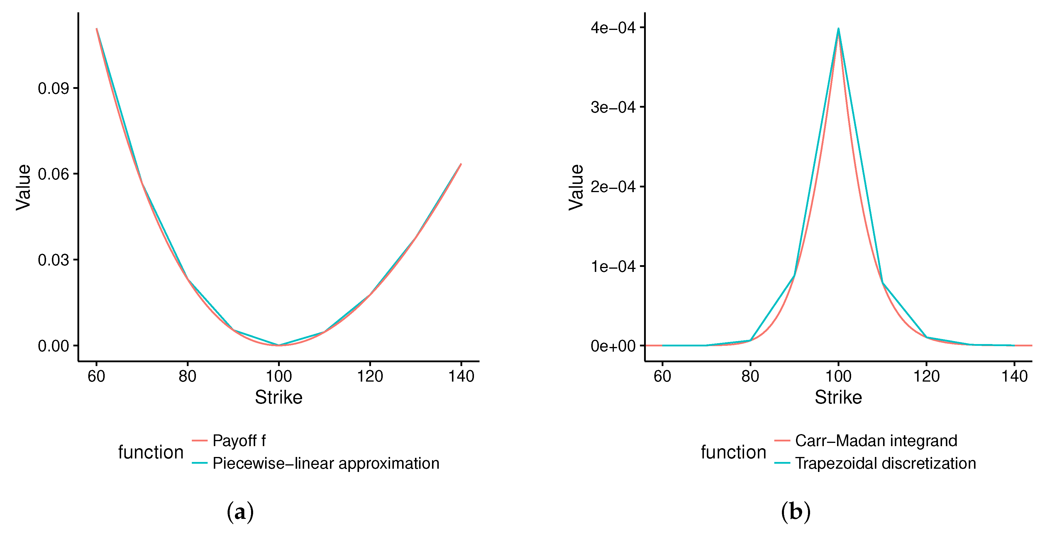
The discretization has a direct impact on the error (

Table 6. Variance swap prices based on SPX500 options under the Heston model parameters from Table 5.

Method	Price	Price in Vol	Error in Vol
Heston	261.44	16.17	0.00
Continuous/Spline	260.51	16.14	0.03
Continuous/Andreasen–Huge	261.03	16.16	0.01
Discrete Cubic Hermite	254.95	15.97	0.20
Discrete Trapezoidal	246.52	15.70	0.47

), even though the range of strikes is relatively dense (78 distinct strikes). With a Hermite-spline discretization of the Carr–Madan integrand represented by Equation (4), the price error is 0.20% compared to a price error under 0.03% for the continuous approach. The choice of market volatility interpolation does not however matter too much in the continuous replication.

6.3. Jumps Effect

Beside the problem of replicating the log contract with vanilla options in practice, another important issue of the variance swap is its difference compared to the log contract assuming jumps (cubic returns cannot be ignored anymore). This is a popular explanation for the single name variance swap market collapse in 2008, as jumps are more pronounced in single name stocks. In the same period, the volatility swap market has increased.

We will see why with the example of the Bates model Bates (1996) as it includes jumps in the asset along with stochastic volatility. In the Bates model, the asset follows:

$$\begin{array}{cc}\hfill \frac{dF}{F}& =-\lambda \overline{k}dt+\sqrt{v}d{W}_F+dZ\hfill \end{array}$$

(29)

$$\begin{array}{cc}\hfill dv& =\kappa (\theta -v)dt+\sigma \sqrt{v}d{W}_v\hfill \end{array}$$

(30)

where $W_F$ and $W_v$ are Brownian motions correlated with correlation $\rho$, $\lambda$ is the annual frequency of jumps, Z is a Poisson process with intensity $\lambda$ and k is the random percentage jump conditional on a jump occurring with the log-normal distribution of jumps sizes $\overline{k}$ such that $ln(1+k)\sim N(ln(1+\overline{k})-\frac{1}{2}{\delta }^2,{\delta }^2)$. $\overline{k}$ thus corresponds to the jump mean, and a higher value will translate to larger jumps, while $\delta$ is the jump volatility. The additional drift term $\lambda \overline{k}$ in Equation (29) comes from the no-arbitrage condition.

Sometimes, the Bates model jump parameters are given according the Merton jump model specification, that is using the parameter $\alpha =ln(1+\overline{k})-\frac{1}{2}{\delta }^2$. Bates parameters lead to a simpler characteristic function, but for the purpose of variance swap and volatility swaps, Merton’s parameters lead to simpler pricing formulae. Under the Bates model, the strike that makes the value of continuously-monitored variance swap zero is Broadie and Jain (2008):

$$K^2=\theta +\frac{v_0-\theta }{\kappa T}\left(1-e^{-\kappa T}\right)+\lambda \left({\alpha }^2+{\delta }^2\right).$$

(31)

To compute the price of a continuously-monitored volatility swap, Broadie and Jain (2008) use the identity:

$$\sqrt{x}=\frac{1}{2\sqrt{\pi }}{\int }_0^{\infty }\frac{1-e^{-sx}}{s^{\frac{3}{2}}}ds$$

(32)

to obtain:

$$K=\frac{1}{2\sqrt{\pi }}{\int }_0^{\infty }\frac{1-e^{A(s)-B(s)v_0+\lambda TC(s)}}{s^{\frac{3}{2}}}ds$$

(33)

with:

$$\begin{array}{cc}\hfill A(s)& =\frac{2\kappa \theta }{{\sigma }^2}ln\frac{2g(s)e^{\frac{1}{2}(g(s)+\kappa )T}}{(g(s)+\kappa )\left(e^{g(s)T}-1\right)+2g(s)},\hfill \end{array}$$

(34)

$$\begin{array}{cc}\hfill B(s)& =\frac{2s\left(e^{g(s)T}-1\right)}{T(g(s)+\kappa )\left(e^{g(s)T}-1\right)+2g(s)T},\hfill \end{array}$$

(35)

$$\begin{array}{cc}\hfill C(s)& =\frac{\sqrt{T}{e}^{-\frac{s{\alpha }^2}{T+2s{\delta }^2}}}{\sqrt{T+2s{\delta }^2}}-1,\hfill \end{array}$$

(36)

$$\begin{array}{cc}\hfill g(s)& =\sqrt{{\kappa }^2+\frac{2s{\sigma }^2}{T}}.\hfill \end{array}$$

(37)

Note that in absence of jumps, that is with $\lambda =0$, Equation (3) also corresponds to the price of a zero coupon under the Cox–Ingersoll–Ross (CIR) model Gatheral (2006). Written as is, Equation (3) does not behave well numerically since the integrand explodes around zero. The variable transformation $y=s^2$ allows restoring a good behavior around zero; we then have:

$$K=\frac{1}{\sqrt{\pi }}{\int }_0^{\infty }\frac{1-e^{A(y^2)-B(y^2)v_0+\lambda TC(y^2)}}{y^2}dy$$

(38)

and:

$$\begin{array}{cc}\hfill \underset{y\to 0}{lim}\frac{1-e^{A(y^2)-B(y^2)v_0+\lambda TC(y^2)}}{s^2}& =\theta +\lambda \left({\alpha }^2+{\delta }^2\right)+\frac{\theta -v_0}{\kappa T}\left(e^{-\kappa T}-1\right),\hfill \end{array}$$

(39)

$$\begin{array}{cc}\hfill \frac{1-e^{A(y^2)-B(y^2)v_0+\lambda TC(y^2)}}{s^2}& \sim \frac{1}{y^2}\mathrm{as}y\to \infty .\hfill \end{array}$$

(40)

We consider three sets of Bates parameters: the first one is a somewhat extreme example where jumps are very pronounced, and their effect easily observable; the second one is the result of a calibration of the Eurostoxx 50 index on October 2003 by Schoutens et al. (2003); and the third one is the result of the calibration against S&P500 option prices on 2 November 1993 by Broadie and Jain (2008) (

Table 7. Bates parameters.

Name	${\mathit{v}}_0$	$\mathit{\kappa }$	$\mathit{\theta }$	$\mathit{\sigma }$	$\mathit{\rho }$	$\mathit{\lambda }$	$\overline{\mathit{k}}$	$\mathit{\delta }$
Extreme	0.04	1.15	0.04	0.39	$-0.64$	0.6	$-0.12$	0.15
Schoutens et al.	0.0576	0.4963	0.2286	0.0650	$-0.99$	0.1382	0.1791	0.1346
Broadie and Jain	0.00988	3.99	0.014	0.27	$-0.79$	0.11	$-0.12$	0.15

). We also assume zero interest and dividend rates. From those parameters, we compute a dense set of vanilla option prices of a maturity of one year, which will be used for replication-based or local volatility-based pricing. The local volatility model offers an alternative to the model-independent Carr–Lee replication, which will also take into account the volatility smile and not the jumps and is commonly used to price exotics Windcliff et al. (2006).

In order to compare the value of the variance (respectively volatility) swap under the Bates model with the value of the same variance or volatility swap under the Dupire local volatility model Dupire (1994), we rely on a Monte Carlo simulation of each model with daily time steps, as there is no closed-form formula or simple quadrature technique to compute the price of a volatility swap under the local volatility model. As an indication, we also give the prices of the continuously-monitored variance and volatility swaps using the closed-form formulae for the Bates model, as well as the continuous replication formula for the variance swap and the Carr–Lee correlation-immune replication for the volatility swap Carr and Lee (2008).

Table 8. Evolution of variance swap prices under extreme Bates parameters, varying the jump parameters.

Parameters	$\mathit{\lambda }=0$	$\mathit{\lambda }=0.6$
		$\overline{\mathit{k}}=-0.12$	$\overline{\mathit{k}}=-0.24$	$\overline{\mathit{k}}=-0.48$
Bates	400.0	651.1	1024.7	3189.8
Replication	400.0	629.0	948.3	2612.9
Relative difference	0.0%	−3.39%	−7.46%	−18.09%
Monte Carlo
Bates	399.0	655.3	1033.0	3205
Local volatility	398.3	626.1	943.3	2577
Relative difference	−0.18%	−4.46%	−8.68%	−19.59%

shows that the local volatility Monte Carlo prices are very close to the continuous replication prices, and the Bates Monte Carlo prices are very close to the closed-form formulae. The effect of the discreteness of the observations is small, and our Monte Carlo simulation is accurate.

In theory, when there are no jumps ($\lambda =0$), the variance swap prices should be the same under local volatility and Bates models as the variance swap payoff can be perfectly replicated by a continuous stream of vanilla options. We can see that when the jump mean $\overline{k}$ increases, the difference in the variance swap prices computed with Bates and local volatility increases by the same scale: the variance swap contract is indeed very dependent on jumps (Table 8).

Under the extreme parameter set, the volatility swap is slightly less influenced by jumps, and more importantly, the effect of jumps is opposite: assuming jumps in the model decrease the price of a volatility swap (

Table 9. Evolution of volatility swap prices under extreme Bates parameters, varying the jump parameters.

Parameters	$\mathit{\lambda }=0$	$\mathit{\lambda }=0.6$
		$\overline{\mathit{k}}=-0.12$	$\overline{\mathit{k}}=-0.24$	$\overline{\mathit{k}}=-0.48$
Bates	18.74	23.35	28.22	45.63
Carr–Lee	18.56	24.16	30.20	51.61
Relative difference	−0.8%	3.64%	7.26%	13.30%
Monte Carlo
Bates	18.69	23.37	28.28	45.7
Local volatility	19.38	24.48	29.94	48.7
Relative difference	3.69%	4.75%	5.87%	6.56%

). Note that without jump, the price under local volatility and the price under Bates are different, as contrary to the variance swap, the volatility swap cannot be exactly statically replicated.

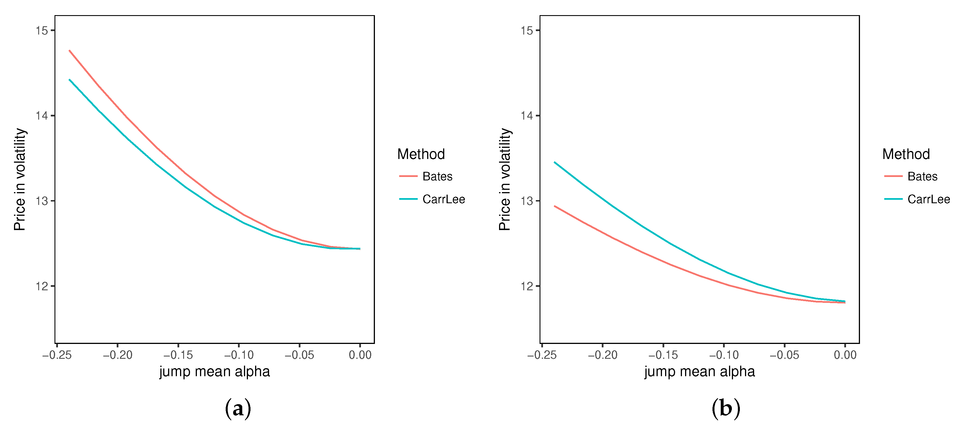
The jump mean is of opposite sign in the parameter set from Schoutens et al. (2003), and now, the continuous replication overestimates the price of the variance swap (Figure 2a).

The price of the volatility swap under continuous replication increases as much as the price of the variance swap, while at the same time, the theoretical (Bates) volatility swap price increases less. With the Schoutens et al. parameters, the volatility swap replication is more sensitive to jumps than the variance swap, even though the actual theoretical volatility swap price is less sensitive to jumps.

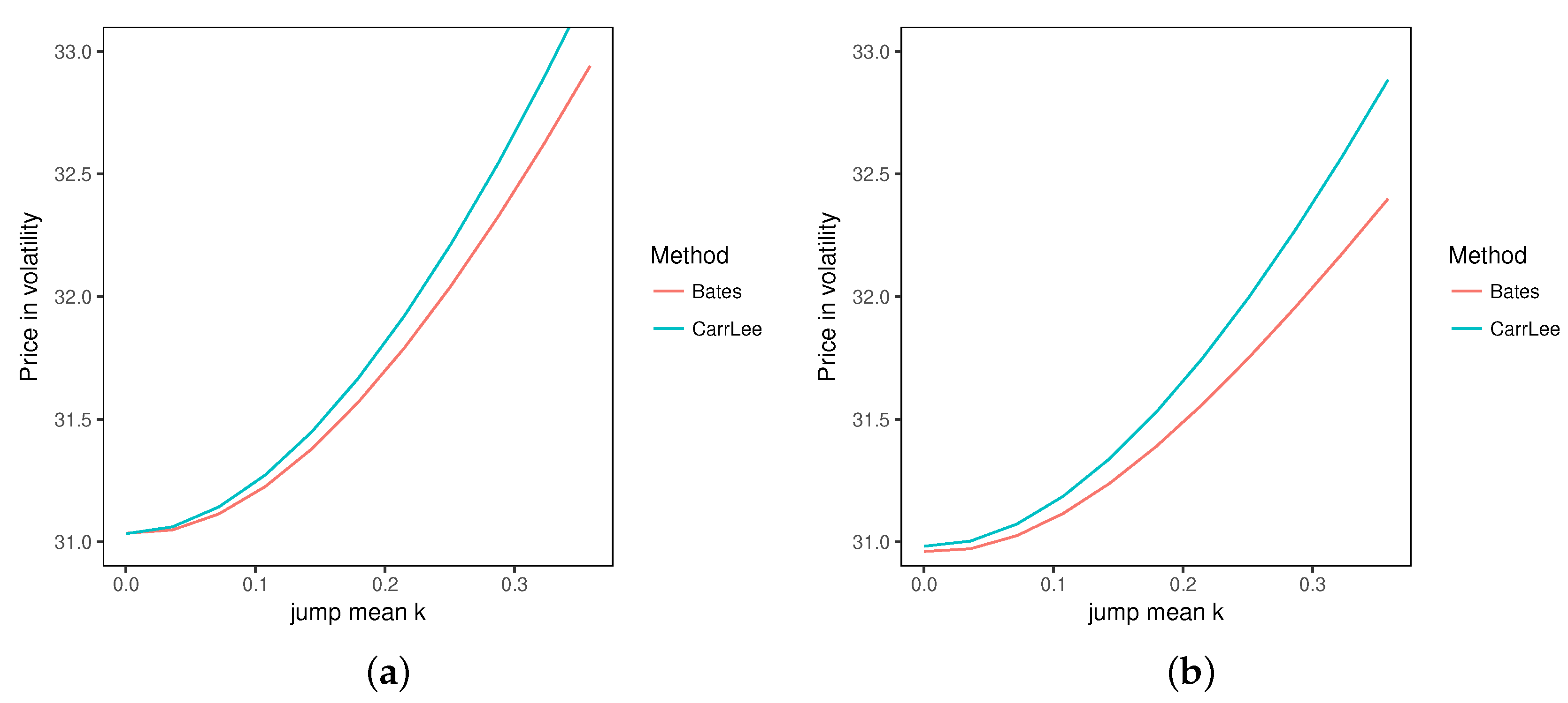
With the parameters from Broadie and Jain (2008), the jump mean is negative, and as expected, the variance swap replication underestimates the theoretical variance swap value, while the volatility swap replication will overestimate the theoretical volatility swap value when the size of the jump increases (Figure 3b).

The replication price can be seen as the price when there is no jump, using the implied volatilities (or equivalently, option prices) from the Bates model with jumps. This allows easily comparing on one side the effect of the jump mean on the theoretical volatility and variance swaps prices and on the other side the effect of the jump assumption on the volatility and variance swap prices. While overall, the volatility swap is less sensitive to the jump mean than the variance swap, it is more sensitive to the assumption of jumps, as the spread between the replication and the theoretical value becomes larger when the jump size increases in mean absolute value. In fact, a rough approximation on Ito’s lemma for semi-martingales suggests that the volatility swap replication error is quadratic with the jump size, as contrary to the variance swap case, the quadratic term does not cancel out (see Carr and Wu (2008)).

Contrary to what is suggested in Carr and Wu (2008), we find that the jumps have a sizeable effect on the prices of both variance and volatility swaps under the Bates model calibrated to different markets, possibly because they explore the 30-day volatility, while we look at the one-year effect.

7. Conclusions

A discrete replication can be useful to obtain an estimate of how much a hedge of a variance swap would cost. However, we have seen that there exists different possible strategies, and those can lead to relatively different hedging prices. More importantly, typical discrete replications significantly underestimate tail events. This leads to an artificially low variance swap price and invalidates the simple discrete hedging strategy effectiveness in practice. Finally, we have shown through the example of the Bates model that this can be compounded with the effect of jumps: discrete or continuous replication assumes no jumps and will again underestimate the price in cases of jumps with negative mean size. In contrast, the volatility swap is less sensitive to tail events. Its replication overvalues the price regardless of the jump mean size sign, while the variance swap replication overvalues the price with jumps of positive mean size and undervalues with jumps of negative mean size.

References

1. Andreasen, Jesper, and Brian Norsk Huge. 2010. Volatility interpolation. Available online: https://ssrn.com/abstract=1694972 or http://dx.doi.org/10.2139/ssrn.1694972 (accessed on 1 July 2016).
2. Bates, David S. 1996. Jumps and stochastic volatility: Exchange rate processes implicit in deutsche mark options. Review of Financial Studies 9: 69–107. [Google Scholar] [CrossRef]
3. Broadie, Mark, and Ashish Jain. 2008. The effect of jumps and discrete sampling on volatility and variance swaps. International Journal of Theoretical and Applied Finance 11: 761–97. [Google Scholar] [CrossRef]
4. Carr, Peter, and Dilip Madan. 2001. Towards a theory of volatility trading. In Option Pricing, Interest Rates and Risk Management, Handbooks in Mathematical Finance. Cambridge: University Press, pp. 458–76. [Google Scholar]
5. Carr, Peter, and Keith Lewis. 2004. Corridor variance swaps. Risk Magazine 17: 67–72. [Google Scholar]
6. Carr, Peter, and Liuren Wu. 2008. Variance risk premiums. The Review of Financial Studies 22: 1311–41. [Google Scholar] [CrossRef]
7. Carr, Peter, and Roger Lee. 2007. Realized volatility and variance: Options via swaps. Risk 20: 76–83. [Google Scholar]
8. Carr, Peter, and Roger Lee. 2008. Robust Replication of Volatility Derivatives. Available online: http://www.cims.nyu.edu/working_paper_series (accessed on 1 July 2016).
9. Dupire, Bruno. 1994. Pricing with a smile. Risk 7: 18–20. [Google Scholar]
10. Demeterfi, Kresimir, Emanuel Derman, Michael Kamal, and Joseph Zou. 1999. More than you ever wanted to know about volatility swaps. Goldman Sachs Quantitative Strategies Research Notes 41: 1–56. [Google Scholar]
11. Espelid, Terje O. 2003. Doubly adaptive quadrature routines based on Newton—Cotes rules. BIT Numerical Mathematics 43: 319–37. [Google Scholar] [CrossRef]
12. Fukasawa, Masaaki, Isao Ishida, Nabil Maghrebi, Kosuke Oya, Masato Ubukata, and Kazutoshi Yamazaki. 2011. Model-free implied volatility: from surface to index. International Journal of Theoretical and Applied Finance 14: 433–63. [Google Scholar] [CrossRef]
13. Gatheral, Jim. 2004. A Parsimonious Arbitrage-Free Implied Volatility Parameterization with Application to the Valuation of Volatility Derivatives. Presentation at Global Derivatives & Risk Management. Madrid: Merrill Lynch. [Google Scholar]
14. Gatheral, Jim. 2006. The Volatility Surface: A Practitioner’s Guide. Hoboken: Wiley, vol. 357. [Google Scholar]
15. Gander, Walter, and Walter Gautschi. 2000. Adaptive quadrature revisited. BIT Numerical Mathematics 40: 84–101. [Google Scholar] [CrossRef]
16. Heston, Steven L. 1993. A closed-form solution for options with stochastic volatility with applications to bond and currency options. Review of Financial Studies 6: 327–43. [Google Scholar] [CrossRef]
17. Jiang, George J., and Yisong S. Tian. 2005. The model-free implied volatility and its information content. The Review of Financial Studies 18: 1305–42. [Google Scholar] [CrossRef]
18. Jiang, George J., and Yisong S. Tian. 2007. Extracting model-free volatility from option prices: An examination of the VIX index. The Journal of Derivatives 14: 35–60. [Google Scholar] [CrossRef]
19. Leung, Tim, and Matthew Lorig. 2016. Optimal static quadratic hedging. Quantitative Finance 16: 1341–55. [Google Scholar] [CrossRef]
20. Schoutens, Wim, Erwin Simons, and Jurgen Tistaer. 2003. A perfect calibration! Now what? In The best of Wilmott. Hoboken: Wiley, p. 281. [Google Scholar]
21. Windcliff, Heath A., Peter A. Forsyth, and Kenneth R. Vetzal. 2006. Pricing methods and hedging strategies for volatility derivatives. Journal of Banking & Finance 30: 409–31. [Google Scholar]
Figure 1. Different replications using Strikes 60–140 by an increment of 10 for a forward F ( 0 , T ) = 100 . (a) Derman’s method: payoff from Equation (11) vs. its piecewise linear approximation; (b) trapezoidal method: integrand of Equation (4) vs. its trapezoidal discretization.
Jrfm 11 00011 g001
Figure 2. Effect of jumps on the price of variance and volatility swaps using the Bates parameters from Schoutens et al. (2003). (a) Variance swap prices; (b) volatility swap prices.
Jrfm 11 00011 g002
Figure 3. Effect of jumps on the price of variance and volatility swaps using the Bates parameters from Broadie and Jain (2008). (a) Variance swap prices; (b) volatility swap prices.
Jrfm 11 00011 g003