Article

GARCH Modelling of Cryptocurrencies

1
School of Mathematics, University of Manchester, Manchester M13 9PL, U.K.
2
Department of Mathematics and Statistics, American University of Sharjah, Sharjah P.O. Box 26666, UAE
3
School of Engineering, Zurich University of Applied Sciences, 8400 Winterthur, Switzerland
*
Author to whom correspondence should be addressed.
J. Risk Financial Manag. 2017, 10(4), 17; https://doi.org/10.3390/jrfm10040017
Submission received: 31 August 2017 / Revised: 27 September 2017 / Accepted: 28 September 2017 / Published: 1 October 2017
(This article belongs to the Special Issue Extreme Values and Financial Risk)

Abstract

:
With the exception of Bitcoin, there appears to be little or no literature on GARCH modelling of cryptocurrencies. This paper provides the first GARCH modelling of the seven most popular cryptocurrencies. Twelve GARCH models are fitted to each cryptocurrency, and their fits are assessed in terms of five criteria. Conclusions are drawn on the best fitting models, forecasts and acceptability of value at risk estimates.

1. Introduction

A cryptocurrency can be defined as “a digital asset designed to work as a medium of exchange using cryptography to secure the transactions and to control the creation of additional units of the currency”. In recent years, the popularity and use of cryptocurrencies has increased dramatically. For example, the U.K. government is looking at Bitcoin technology (Bitcoin is the first and the most popular cryptocurrency) for tracking taxpayer money. The U.S. government is to sell over 44,000 Bitcoins.
Because of this increasing interest, there is a need to quantify the variation of cryptocurrencies. It is well known that cryptocurrencies are highly volatile compared to traditional currencies. Certainly, their exchange rates cannot be assumed to be independently and identically distributed. Perhaps the most popular models for the exchange rates of traditional currencies are based on Generalized Autoregressive Conditional Heteroskedasticity (GARCH) models. However, there exists little work on fitting of GARCH-type models to the exchange rates of cryptocurrencies. The known work focuses on GARCH modelling of Bitcoin, the first and the most popular cryptocurrency.
Katsiampa (2017) estimated the volatility of Bitcoin through a comparison of GARCH models, and the AR-CGARCH model was shown to give the optimal fit. Urquhart (2017) illustrated that HARmodels are more robust in modelling Bitcoin volatility than traditional GARCH models. Stavroyiannis and Babalos (2017) examined dynamic properties of Bitcoin modelling through univariate and multivariate GARCH models and vector autoregressive specifications. Cermak (2017) used a GARCH (1, 1) to model Bitcoin’s volatility with respect to macroeconomic variables, in countries where Bitcoin has the highest volume of trading. The results showed that Bitcoin behaves similarly to fiat currencies in China, the U.S. and Europe, but not in Japan. In particular, Bitcoin appeared to be an attractive asset for investment and store of value in China; Bouoiyour and Selmi (2015, 2016) analysed daily Bitcoin prices using an optimal-GARCH model and showed that the volatility has decreased when comparing data from 2010–2015 with data from the first half of 2015. The asymmetry in the Bitcoin market was still significant, suggesting that Bitcoin prices were driven more by negative than positive shocks; Chen et al. (2016) provided an econometric analysis of the CRIXindex family using data from 2014–2016. Using a variety of GARCH models, they found that the TGARCH (1, 1) model is the best fitting model for all sample data based on discrimination criteria such as the log likelihood, AIC and BIC. In addition, the DCC-GARCH (1, 1) was found to show volatility clustering and time varying covariances between three CRICindices; Letra (2016) used a GARCH (1, 1) model to analyse daily Bitcoin prices and search trends on Google, Wikipedia and tweets on Twitter. They found that Bitcoin prices were influenced by popularity, but also that web content and Bitcoin prices had some predictable power. Dyhrberg (2016a) applied the asymmetric GARCH methodology to explore the hedging capabilities of Bitcoin. It was shown that Bitcoin can be used as a hedge against stocks in the Financial Times Stock Exchange Index and against the American dollar in the short term. Dyhrberg (2016b) used GARCH models to explore the financial asset capabilities of Bitcoin. It was shown that Bitcoin has a place on the financial markets and in portfolio management as it can be classified as something in between gold and the American dollar, on a scale from pure medium of exchange advantages to pure store of value advantages. Bouri et al. (2017) used asymmetric GARCH models to investigate the relationship between price returns and volatility changes in the Bitcoin market around the price crash of 2013.
The aim of this paper is to provide GARCH-type modelling of the seven most popular cryptocurrencies. They are Bitcoin, Dash, Dogecoin, Litecoin, Maidsafecoin, Monero and Ripple. We fit twelve different GARCH-type models to the log returns of the exchange rates of each of these cryptocurrencies. The method of maximum likelihood was used for fitting. The goodness of fit was assessed in terms of five different criteria. Conclusions are drawn on the best fitting GARCH models, forecasts based on them and the ability of the models to estimate value at risk.
The contents of the paper are organized as follows. Section 2 describes the data used and some summary statistics of the data described. Section 3 describes the GARCH-type models fitted and the criteria used to assess their goodness of fit. The results of fitting the models and their discussion are given in Section 4. Finally, some conclusions are noted in Section 5.

2. Data

The data that we used in our analysis were the historical daily global price indices of particular cryptocurrencies and were extracted from the BNC2database from Quandl. In order to obtain the most accurate prices, the global indices were used as they are computed by using a weighted average of the price of each cryptocurrency, using prices from a number of different exchanges, as in Chan et al. (2017). Although our daily data begin only one day earlier than those in Chan et al. (2017), 22 June 2014, the end date is much later, on 17 May 2017. We obtained more up to date data for our analysis so that we could again analyse seven of the top fifteen cryptocurrencies, ranked by market capitalization, in May 2017. The most up to date (daily) market capitalization figures for all cryptocurrencies can be found online; see CoinMarketCap (2017). In May 2017, the top seven cryptocurrencies ranked by market capitalization were the same as those in February 2017 (Chan et al. (2017)) and include Bitcoin, Dash, LiteCoin, MaidSafeCoin, Monero, DogeCoin and Ripple. Other notable cryptocurrencies such as Ethereum, Ethereum Classic, Agur and NEMwere omitted due to the volume of available data. It should be noted that in May 2017, the seven cryptocurrencies represented 90 percent of the total market capitalization. However, due to the volatility of cryptocurrencies, the rankings of the respective cryptocurrencies has since changed. For a brief description of the seven cryptocurrencies, see Chan et al. (2017).
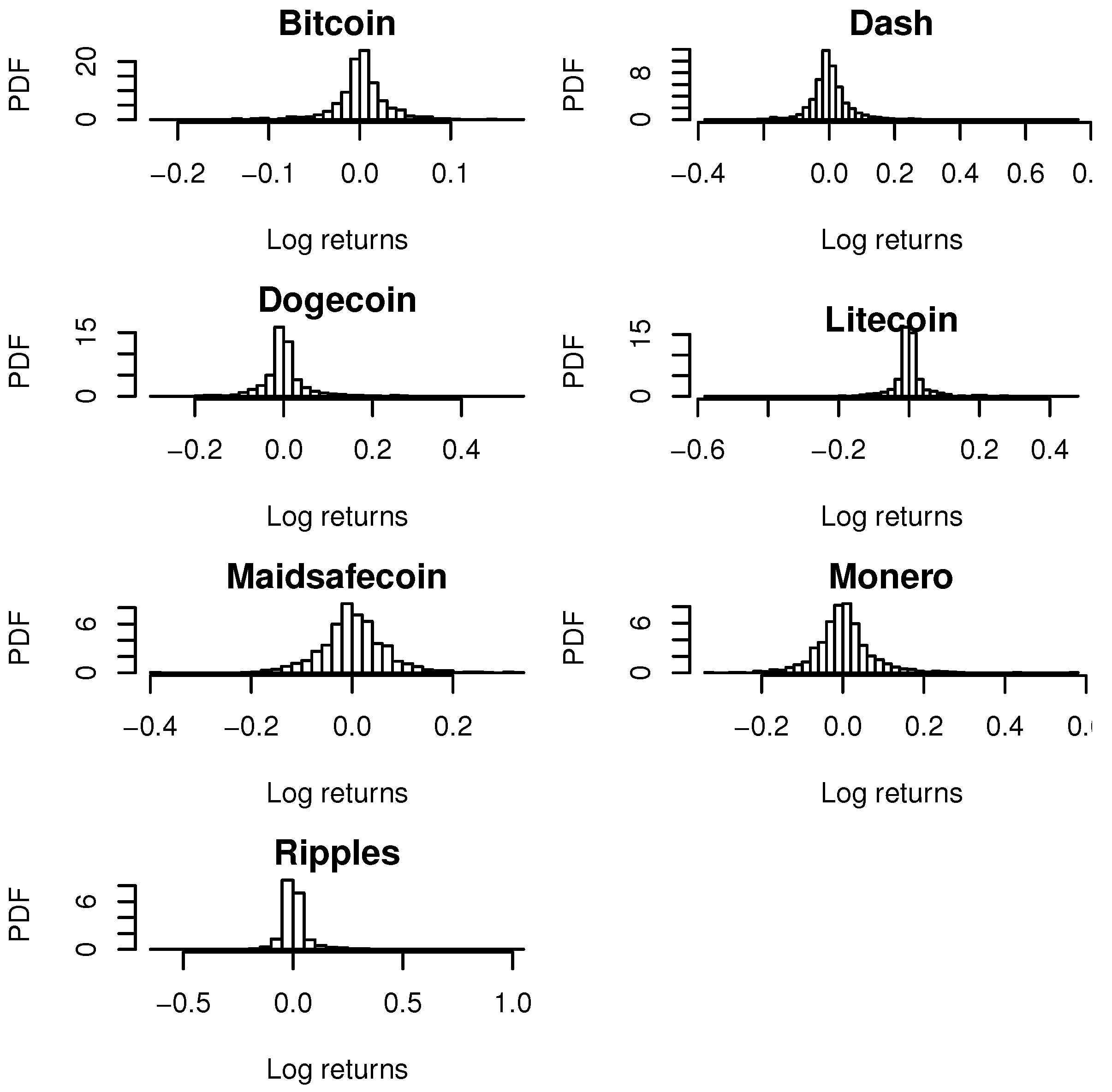
The summary statistics are the largest for Bitcoin, followed by Dash, Litecoin, Monero, Ripple, Maidsafecoin and Dogecoin (Table 1). The log returns for each cryptocurrency are positively skewed. The log returns are heavy tailed with kurtosis greater than that of the normal distribution for Bitcoin, Dash, Litecoin and Ripple. The log returns are light tailed with kurtosis less than that of the normal distribution for Dogecoin, Maidsafecoin and Monero.
Figure 1 shows the histograms of the log returns of the daily market price indices for all exchanges trading in Bitcoin, Dash, Dogecoin, Litecoin, Maidsafecoin, Monero and Ripple. From the plots, we find that the log returns are more or less symmetrically distributed. Some histograms appear more peaked than others.

3. Models

First, we provide an introduction to twelve GARCH type models used to analyse our cryptocurrency datasets: SGARCH, EGARCH, GJRGARCH, APARCH, IGARCH, CSGARCH, GARCH, TGARCH, AVGARCH, NGARCH, NAGARCHand ALLGARCH models. Secondly, criteria used to selected the best fitting models are given. Thirdly, formulas are provided for estimating value at risk based on the fitted models.

3.1. GARCH Models

Let X t denote the observed financial data series; in our case, these are the log returns of the prices of the respective cryptocurrencies. Then, GARCH models can be specified as:
X t = μ t + σ t Z t ,
where μ t denotes the conditional mean and σ t denotes a volatility process. All of the GARCH-type models used follow the above specification in (1); however, in each case, the volatility process σ t is different. For simplicity, we restrict all of the models to a maximum order of one. In addition, for each GARCH-type model, the innovation process Z t is allowed to follow one of eight distributions; these are the normal distribution, skew normal distribution (Azzalini (1985)), Student’s t distribution (Gosset (1908)), skew Student’s distribution (Fernandez and Steel (1998)), skew generalized error distribution (Theodossiou (1998)), generalized hyperbolic distribution Barndorff-Nielsen (1977; 1978) normal inverse Gaussian distribution Barndorff-Nielsen (1977, 1978) and Johnson’s SU distribution (Johnson (1949)).
The standard GARCH model (Bollerslev (1986)), denoted by SGARCH (1, 1), has:
σ t 2 = ω + α 1 Z t 1 2 + β 1 σ t 1 2
for α 1 > 0 , β 1 > 0 and ω > 0 . The main feature of this and other models is that they capture volatility clustering in the data. The “persistence” parameter (which accounts for the amount of volatility clustering captured by the model) for this model is α 1 + β 1 . Weak stationarity holds if α 1 + β 1 < 1 .
The integrated GARCH model (Engle and Bollerslev (1986)), denoted by IGARCH (1, 1), is a particular case of the SGARCH (1, 1) model for α 1 + β 1 = 1 . That is, the persistence parameter is equal to one. This model is strictly stationary.
The exponential GARCH model (Nelson (1991)), denoted by EGARCH (1, 1), has:
log σ t 2 = ω + α 1 Z t 1 + γ 1 Z t 1 E Z t 1 + β 1 log σ t 1 2
for α 1 > 0 , β 1 > 0 , γ 1 > 0 and ω > 0 . α 1 captures the sign effect, and γ 1 captures the size effect. The persistence parameter for this model is β 1 . A difference from SGARCH (1, 1) is that the conditional variance is written as a function of the past standardized innovations, instead of the past innovations. A one line derivation of the EGARCH (1, 1) is described in McAleer and Hafner (2014).
The GJRGARCH (1, 1) model due to Glosten et al. (1993) has:
σ t 2 = ω + α 1 Z t 1 2 + γ 1 I t 1 Z t 1 2 + β 1 σ t 1 2
for α 1 > 0 , β 1 > 0 , γ 1 > 0 and ω > 0 , where I t 1 = 1 if Z t 1 0 and I t 1 = 0 if Z t 1 > 0 . GJRGARCH (1, 1) is an asymmetric version of SGARCH (1, 1), reflects the asymmetric nature of investor response to stock and index returns and leads to positive and negative shocks having different effects on the conditional volatility. γ 1 represents an asymmetry parameter. A positive shock will increase volatility by α 1 at t; a negative shock will increase volatility by α 1 + γ 1 at t. The persistence depends on this parameter through α 1 + β 1 + γ 1 κ , where κ denotes the expected value of the standardized residuals.
In both the EGARCH (1, 1) and GJRGARCH (1, 1) models, asymmetry arises if γ 1 > 0 (McAleer (2014)), so they both always display asymmetry. Leverage is not possible in either the EGARCH (1, 1) or GJRGARCH (1, 1) model (McAleer (2014); Chang and McAleer (2017)).
The ALL GARCH (1, 1) model due to Hentschel (1995) has:
σ t δ = ω + α 1 σ t 1 δ Z t 1 η 1 γ 1 Z t 1 η 1 δ + β 1 σ t 1 δ
for δ > 0 , α 1 0 , β 1 0 , 1 < γ 1 < 1 , < η 1 < and ω > 0 . δ is a parameter for the Box–Cox transformation. The persistence parameter is equal to β 1 + α 1 κ 1 , where κ 1 is the expected value of the standardized residuals under the Box–Cox transformation of the absolute value of the asymmetry term. The ALLGARCH(1, 1) model contains the following as particular cases: the NAGARCH (1, 1) model of Engle and Ng (1993) for δ = 2 and γ 1 = 0 ; the GARCH (1, 1) model of Bollerslev (1986) for δ = 2 and γ 1 = η 1 = 0 ; the GJRARCH (1, 1) model of Glosten et al. (1993) for δ = 2 and η 1 = 0 ; the TGARCH (1, 1) model of Zakoian (1994) for δ = 1 and η 1 = 0 ; the NGARCH (1, 1) model of Higgins and Bera (1992) for γ 1 = η 1 = 0 ; the APARCH (1, 1) model of Ding et al. (1993) for η 1 = 0 .
The asymmetric power ARCH model (Ding et al. (1993)), denoted by APARCH (1, 1), has:
σ t δ = ω + α 1 Z t 1 γ 1 Z t 1 δ + β 1 σ t 1 δ
for δ > 0 , α 1 0 , β 1 0 , 1 < γ 1 < 1 and ω > 0 . APARCH (1, 1) models for both the leverage and the effect that the sample autocorrelation of absolute returns are usually larger than that of squared returns. δ is a parameter for the Box–Cox transformation, and γ 1 is a leverage parameter. The persistence parameter is equal to β 1 + α 1 κ 1 , where κ 1 is the expected value of the standardized residuals under the Box–Cox transformation of the term, which includes the leverage parameter γ 1 . APARCH (1, 1) contains the following as particular cases: the SGARCH (1, 1) model due to Bollerslev (1986) for δ = 2 and γ 1 = 0 ; the AVGARCH (1, 1) model due to Taylor (1986) and Schwert (1990) for δ = 1 and γ 1 = 0 ; the GJRGARCH (1, 1) model due to Glosten et al. (1993) for δ = 2 ; the NGARCH (1, 1) model due to Higgins and Bera (1992) for β 1 = 0 and γ 1 = 0 .
The TGARCH (1, 1) model due to Zakoian (1994) is the particular case of APARCH (1, 1) for δ = 1 . Therefore, the specification is one on the conditional standard deviation instead of the conditional variance.
The component standard GARCH model (Lee and Engle (1999)), denoted by CSGARCH (1, 1), has:
σ t 2 = q t + α 1 Z t 1 2 q t 1 + β 1 σ t 1 2 q t 1 ,
where:
q t = ω + ρ q t 1 + ϕ Z t 1 2 σ t 1 2
for δ > 0 , α 1 0 , β 1 0 , ϕ 0 and ω > 0 . Weak stationarity holds if α 1 + β 1 < 1 and ρ < 1 . CSGARCH (1, 1) decomposes the conditional variance into permanent and transitory components so as to investigate the long- and short-run movements of volatility. Compared to SGARCH (1, 1), the intercept parameter is now a time-varying first order autoregressive process.
Detailed conditions for stationarity (weak or strict) for several of the GARCH models can be found in: Nelson (1990) (Theorems 1 and 2, p. 320, 1990) for the SGARCH (1, 1) and IGARCH (1, 1) models; Zakoian (1994) (Propositions 2-3, 1994), Francq and Zakoian (2010) (Theorem 10.3 to 10.5, 2010) and Goncalves et al. (2012) (Theorems 5 and 6, 2012) for the TGARCH (1, 1) model; the Appendix in Hentschel (1995) for the ALL GARCH (1, 1) model; Ling and McAleer (2003) (Theorem 2.1, 2003) for the ARMA-GARCH model; Francq and Zakoian (2010) (Theorem 10.1, 2010) and Francq et al. (2013) (Theorem 2.1, p. 36, 2013) for the EGARCH (1, 1) model; Bardet et al. (2017) (Proposition 2.1, p. 456, 2017) for the APARCH (1, 1) model.
Estimators, their consistency and their asymptotic normality have been established for several of the known GARCH models. The estimators include a Gaussian quasi-maximum likelihood estimator for the GARCH (1, 1) model (Theorem 3, p. 580, Lumsdaine (1996)); a quasi-maximum likelihood estimator for the ARMA-GARCH model (Theorems 4.1 and 5.1, Ling and McAleer (2003)); a stable quasi-maximum likelihood estimator for the EGARCH (1, 1) model (Theorem 6, p. 859, Wintenberger (2013)); a restricted normal mixture quasi-maximum likelihood estimator for the TGARCH (1, 1) model (Theorem 2.4, p. 1346, Wang and Pan (2014)); a Laplacian quasi-maximum likelihood estimator for the APARCH (1, 1) model (Theorem 3.3, pp. 457–458, Bardet et al. (2017)). Propositions 4.1 and 4.2 in Martinet and McAleer (2017) derive conditions of invertibility of quasi-maximum likelihood estimators of the EGARCH ( p , q ) model.
Explicit expressions for moments of GARCH models have been derived in: Bollerslev (1986) (Theorem 2, 1986) for the SGARCH (1, 1) model; Nelson (1990) (Theorem 6, p. 326, 1990) for the SGARCH (1, 1) and IGARCH (1, 1) models; Zakoian (1994) (Proposition 7, 1994) for the TGARCH (1, 1) model; Karanasos and Kim (2003) (Theorem 1, pp. 149–150, 2003) and Francq and Zakoian (2010) (Theorem 10.2, 2010) for the EGARCH (1, 1) model.

3.2. Model Selection

All of the GARCH-type models were fitted by the method of maximum likelihood. Many of the fitted models are not nested. Discrimination among them was performed using various criteria:
  • the Akaike information criterion due to Akaike (1974) defined by:
    AIC = 2 k 2 ln L Θ ^ ,
    where k denotes the number of unknown parameters, Θ the vector of the unknown parameters and Θ ^ their maximum likelihood estimates;
  • the Bayesian information criterion due to Schwarz (1978) defined by:
    BIC = k ln n 2 ln L Θ ^ ,
    where n denotes the number of observations;
  • the Consistent Akaike Information Criterion (CAIC) due to Bozdogan (1987) defined by:
    CAIC = 2 ln L Θ ^ + k ln n + 1 ;
  • the corrected Akaike Information Criterion (AICc) due to Hurvich and Tsai (1989) defined by:
    AICc = AIC + 2 k ( k + 1 ) n k 1 ;
  • the Hannan–Quinn criterion due to Hannan and Quinn (1979) defined by:
    HQC = 2 ln L Θ ^ + 2 k ln ln n .
The smaller the values of these criteria, the better the fit. For more discussion on these criteria, see Burnham and Anderson (2004) and Fang (2011).

3.3. Estimation of Value at Risk

Here, we provide formulas for estimating the one day-ahead value at risk (see, for example, Equation (6) in Kinateder and Wagner (2014)) for the eight innovation distributions considered in Section 3.1.
For the normal distribution,
VaR ^ p = μ ^ t + 1 + σ ^ t + 1 Φ 1 ( p ) ,
where Φ ( · ) denotes the cumulative distribution function of the standard normal distribution.
For the skew normal distribution (Azzalini (1985)),
VaR ^ p = μ ^ t + 1 + σ ^ t + 1 F 1 ( p ) ,
where:
F ( x ) = Φ ( x ) 2 T x , α ^
for < x < and < α < , where T ( · , · ) denotes Owen’s T function (Owen (1956)).
For the Student’s t distribution (Gosset (1908)),
VaR ^ p = μ ^ t + 1 + σ ^ t + 1 F 1 ( p ) ,
where:
F ( x ) = x f ( y ) d y
for < x < , where
f ( x ) = 2 Γ ν ^ + 1 2 ν ^ ν ^ 2 Γ ν ^ 2 1 + x 2 ν ^ 2 ν ^ + 1 2
for < x < and ν > 0 .
For the skew Student’s distribution (Fernandez and Steel (1998)),
VaR ^ p = μ ^ t + 1 + σ ^ t + 1 F 1 ( p ) ,
where:
F ( x ) = x f ( y ) d y
for < x < , where:
f ( x ) = 2 Γ ν ^ + 1 2 ν ^ ν ^ 2 ξ ^ + ξ ^ 1 Γ ν ^ 2 1 + ξ ^ 2 x 2 ν ^ 2 ν ^ + 1 2 , if   x < 0 , 1 + x 2 ξ ^ 2 ν ^ 2 ν ^ + 1 2 , if   x 0
for < x < , ν > 0 and ξ > 0 .
For the skew generalized error distribution (Theodossiou (1998)),
VaR ^ p = μ ^ t + 1 + σ ^ t + 1 F 1 ( p ) ,
where:
F ( x ) = x f ( y ) d y
for < x < , where:
f ( x ) = C 1 + k ^ θ ^ k ^ 1 λ ^ k ^ n ^ 2 x k ^ n ^ + 1 k ^ , for   x < 0 , 1 + k ^ θ ^ k ^ 1 + λ ^ k ^ n ^ 2 x k ^ n ^ + 1 k ^ , for   x 0
for < x < , k > 0 , n > 2 and 1 < λ < 1 .
For the generalized hyperbolic distribution Barndorff-Nielsen (1977, 1978),
VaR ^ p = μ ^ t + 1 + σ ^ t + 1 F 1 ( p ) ,
where:
F ( x ) = x f ( y ) d y
for < x < , where
f ( x ) = C 1 + x 2 λ ^ 1 2 K λ ^ 1 2 α ^ 1 + x 2 exp β ^ x
for < x < , < λ < , < α < , < β < , β < α if λ > 0 , β < α if λ = 0 and β α if λ < 0 , where C is a normalizing constant and K ν ( · ) denotes the modified Bessel function of the second kind defined by:
K ν ( x ) = π csc ( π ν ) 2 I ν ( x ) I ν ( x ) , if   ν Z , lim μ ν K μ ( x ) , if   ν Z ,
where I ν ( · ) denotes the modified Bessel function of the first kind of order ν defined by:
I ν ( x ) = k = 0 1 Γ ( k + ν + 1 ) k ! x 2 2 k + ν .
For the normal inverse Gaussian distribution Barndorff-Nielsen (1977, 1978),
VaR ^ p = μ ^ t + 1 + σ ^ t + 1 F 1 ( p ) ,
where:
F ( x ) = x f ( y ) d y
for < x < , where
f ( x ) = C 1 + x 2 λ ^ 1 2 K 1 α ^ 1 + x 2 exp β ^ x
for < x < , < α < , < β < , and β α , where C is a normalizing constant.
For Johnson’s SU distribution (Johnson (1949)),
VaR ^ p = μ ^ t + 1 + σ ^ t + 1 F 1 ( p ) ,
where:
F ( x ) = Φ α ^ + β ^ arcsinh ( x )
for < x < , α > 0 and β > 0 .

4. Results

We fitted SGARCH (1, 1), EGARCH (1, 1), GJRGARCH (1, 1), APARCH (1, 1), IGARCH (1, 1), CSGARCH (1, 1), GARCH (1, 1), TGARCH (1, 1), AVGARCH (1, 1), NGARCH (1, 1), NAGARCH (1, 1) and ALL GARCH (1, 1) models to the log returns of the exchange rates of Bitcoin, Dash, Dogecoin, Litecoin, Maidsafecoin, Monero and Ripple. The distribution of the innovation process were taken to be one of normal distribution, skew normal distribution, Student’s t distribution, skew Student’s t distribution, skew generalized error distribution, normal inverse Gaussian distribution, generalized hyperbolic distribution or Johnson’s SU distribution. The values of AIC, AICc, BIC, HQCand CAICare given in Tables 3–14 in Chu et al. (2017) for the fitted models.
The normal distribution gives the smallest values of AIC, AICc, BIC, HQC and CAIC for each cryptocurrency and each GARCH-type model. There are two exceptions however: for the TGARCH (1, 1) models fitted to Ripple, the skew normal distribution gives the smallest values of AIC, AICc, BIC, HQC and CAIC; for the AVGARCH (1, 1) models fitted to Ripple, the skew normal distribution gives the smallest values of AIC, AICc, BIC, HQC and CAIC.
Hence, the best fitting GARCH-type models are the ones with the innovation process following the normal distribution. The two exceptions are: the best of the TGARCH (1, 1) models fitted to Ripple is the one with the innovation process following the skew normal distribution; the best of the AVGARCH (1, 1) models fitted to Ripple is the one with the innovation process following the skew normal distribution.
Among the twelve best fitting GARCH type models, the IGARCH (1, 1) model with normal innovations gives the smallest values of AIC, AICc, BIC, HQC and CAIC for Bitcoin, Dash, Litecoin, Maidsafecoin and Monero. The GJRGARCH (1, 1) model with normal innovations gives the smallest values of AIC, AICc, BIC, HQC and CAIC for Dogecoin. The GARCH (1, 1) model with normal innovations gives the smallest values of AIC, AICc, BIC, HQC and CAIC for Ripple.
Hence, among all of the GARCH type models fitted, the IGARCH (1, 1) model gives the best fit for Bitcoin, Dash, Litecoin, Maidsafecoin and Monero; the GJRGARCH (1, 1) model gives the best fit for Dogecoin; the GARCH (1, 1) model gives the best fit for Ripple.
Figures 2–13 in Chu et al. (2017) show predicted values for the twenty five days following the end of each dataset. The predictions are given for each of the best fitting GARCH-type model. The predictions given are those based on the fitted model (red) and bootstrapping (black). The curves formed by the blue dots are the 5 percentiles, 25 percentiles, 75 percentiles and 95 percentiles of the bootstrap samples.
We see that the predictions based on the best fitting model and bootstrapping agree well. This is a sign of the goodness of fit of the models. The variation of the bootstrap-based percentile appears largest for Ripple for each GARCH-type model. The variation appears smallest for Bitcoin for each GARCH-type model.
We further checked the goodness of fit of the models by the one-sample Kolmogorov–Smirnov test. The p-values of this test for the seven best fitting SGARCH models were 0.238, 0.107, 0.290, 0.207, 0.228, 0.124 and 0.058. The corresponding p-values for the seven best fitting EGARCH models were 0.148, 0.333, 0.338, 0.116, 0.337, 0.369 and 0.229. The corresponding p-values for the seven best fitting GJRGARCH models were 0.345, 0.306, 0.352, 0.314, 0.286, 0.153 and 0.258. The corresponding p-values for the seven best fitting APARCH models were 0.091, 0.241, 0.109, 0.300, 0.394, 0.364 and 0.115. The corresponding p-values for the seven best fitting IGARCH models were 0.197, 0.118, 0.166, 0.207, 0.377, 0.238 and 0.370. The corresponding p-values for the seven best fitting CSGARCH models were 0.136, 0.298, 0.100, 0.073, 0.366, 0.167 and 0.279. The corresponding p-values for the seven best fitting GARCH models were 0.183, 0.217, 0.103, 0.236, 0.142, 0.392 and 0.129. The corresponding p-values for the seven best fitting TGARCH models were 0.087, 0.214, 0.280, 0.317, 0.219, 0.080 and 0.297. The corresponding p-values for the seven best fitting AVGARCH models were 0.071, 0.377, 0.210, 0.136, 0.120, 0.050 and 0.240. The corresponding p-values for the seven best fitting NGARCH models were 0.375, 0.231, 0.207, 0.139, 0.118, 0.236 and 0.341. The corresponding p-values for the seven best fitting NAGARCH models were 0.053, 0.267, 0.312, 0.281, 0.211, 0.051 and 0.335. The corresponding p-values for the seven best fitting ALLGARCH models were 0.241, 0.067, 0.304, 0.078, 0.155, 0.184 and 0.072. Hence, all of the best fitting models provide adequate fits at least at the five percent significance level.
Finally, we perform the unconditional and conditional coverage value at risk exceedances tests (Christoffersen (1998); Christoffersen et al. (2001)). The p-values of the unconditional test for the best fitting models and various exceedance probabilities are given in Table 2, Table 3, Table 4, Table 5, Table 6, Table 7 and Table 8. The corresponding p-values of the conditional test are given in the same tables. All of the p-values are significant at the five percent level of significance. Hence, the best fitting models can be used to provide acceptable estimates of value at risk.

5. Conclusions

We find that the IGARCH and GJRGARCH models provide the best fits, in terms of modelling of the volatility in the most popular and largest cryptocurrencies. The IGARCH model falls within the standard GARCH framework and contains a conditional volatility process, which is highly persistent (with infinite memory), and this has been shown in the literature (Caporale et al. (2003)). However, although the IGARCH (1, 1) with normal innovations appears to give a good fit for numerous cryptocurrencies, it has been shown that this could stem from a structural change in the data, which may not be accounted for; i.e., a policy change (Caporale et al. (2003)). Therefore, more in depth analysis of the datasets may be required to confirm or deny possible structural change.
Due to the increasing demand and interest in cryptocurrencies, we believe that they should now be treated as more than just a novelty. Some cryptocurrencies have recently seen more growth than others, for example, Bitcoin, Ethereum, Litecoin and Ripple. However, there is still much discussion about whether cryptocurrencies, especially Bitcoin, should be classed as currencies, assets or investment vehicles, and this is a key topic in itself. Our analysis assumes that we are looking at cryptocurrencies in terms of financial assets, where most users are trading them for investment purposes: either as a long-term investment in new technology or looking to make a short-term profit. Investigating the volatility of cryptocurrencies is important in terms of financial investment like hedging or pricing instruments. Therefore, these results would be particularly useful in terms of portfolio and risk management and could help others make better informed decisions with regard to financial investments and the potential benefits and pitfalls of utilizing cryptocurrencies.
Our results show that cryptocurrencies such as Bitcoin, Ethereum, Litecoin and many others exhibit extreme volatility especially when we look at their inter-daily prices. This is suited for risk-seeking investors looking for a way to invest or enter into technology markets. Our results can also assist financial institutions.
Regulations and policies surrounding cryptocurrencies are being gradually tightened up by many countries; most recently, the U.S. Securities and Exchange Commission (SEC) has initiated plans to regulate the cryptocurrency exchange and all digital currencies. With the exponential growth of the initial coin offering to raise funds for start ups, we have seen China and South Korea (the biggest markets for cryptocurrencies) already regulating and banning such products. Overall, we believe in implementing more regulations and policy for cryptocurrencies as people are starting to see them as investment prospects.
A future work is to fit multivariate GARCH-type models to describe the joint behaviour of the exchange rates of Bitcoin, Dash, Dogecoin, Litecoin, Maidsafecoin, Monero and Ripple. This will require methodological, as well as empirical developments. Furthermore, we have used value at risk since it has been the most popular risk measure in finance. However, there is a shift of value at risk to stressed expected shortfall in the new Basel III regulation (see, for example, Kinateder (2016)). Therefore, another future work is to use expected shortfall instead of value at risk.

Acknowledgments

The authors would like to thank the Editor and the three referees for careful reading and comments, which greatly improved the paper.

Conflicts of Interest

The authors declare no conflict of interest.

References

  1. Akaike, Hirotugu. 1974. A new look at the statistical model identification. IEEE Transactions on Automatic Control 19: 716–23. [Google Scholar] [CrossRef]
  2. Azzalini, A. 1985. A class of distributions which includes the normal ones. Scandinavian Journal of Statistics 12: 171–78. [Google Scholar]
  3. Bardet, Jean-Marc, Yakoub Boularouk, and Khedidja Djaballah. 2017. Asymptotic behaviour of the Laplacian quasi-maximum likelihood estimator of affine causal processes. Electronic Journal of Statistics 11: 452–79. [Google Scholar] [CrossRef]
  4. Barndorff-Nielsen, Ole E. 1977. Exponentially decreasing distributions for the logarithm of particle size. Proceedings of the Royal Society of London A: Mathematical and Physical Sciences 353: 401–9. [Google Scholar] [CrossRef]
  5. Barndorff-Nielsen, Ole E. 1978. Hyperbolic distributions and distributions on hyperbolae. Scandinavian Journal of Statistics 5: 151–57. [Google Scholar]
  6. Bollerslev, Tim. 1986. Generalized autoregressive conditional heteroskedasticity. Journal of Econometrics 31: 307–27. [Google Scholar] [CrossRef]
  7. Bouoiyour, Jamal, and Refk Selmi. 2015. Bitcoin Price: Is it Really That New Round of Volatility Can Be on Way? MPRA Paper No. 65580. CATT, University of Pau, Pau, France. [Google Scholar]
  8. Bouoiyour, Jamal, and Refk Selmi. 2016. Bitcoin: A beginning of a new phase? Economics Bulletin 36: 1430–40. [Google Scholar]
  9. Bouri, Elie, Georges Azzi, and Anne Haubo Dyhrberg. 2017. On the return-volatility relationship in the Bitcoin market around the price crash of 2013. Economics: The Open-Access, Open-Assessment E-Journal 11: 1–16. [Google Scholar] [CrossRef]
  10. Bozdogan, Hamparsum. 1987. Model selection and Akaike’s Information Criterion (AIC): The general theory and its analytical extensions. Psychometrika 52: 345–70. [Google Scholar] [CrossRef]
  11. Burnham, Kenneth P., and David R. Anderson. 2004. Multimodel inference: Understanding AIC and BIC in model selection. Sociological Methods and Research 33: 261–304. [Google Scholar] [CrossRef]
  12. Caporale, Guglielmo Maria, Nikitas Pittis, and Nicola Spagnolo. 2003. IGARCH models and structural breaks. Applied Economics Letters 10: 765–68. [Google Scholar] [CrossRef]
  13. Cermak, Vavrinec. 2017. Can Bitcoin become a viable alternative to fiat currencies? An empirical analysis of Bitcoin’s volatility based on a GARCH model. Available online: https://ssrn.com/abstract=2961405 (accessed on 30 September 2017).
  14. Chan, Stephen, Jeffrey Chu, Saralees Nadarajah, and Joerg Osterrieder. 2017. A statistical analysis of cryptocurrencies. Journal of Risk Financial Management 10: 12. [Google Scholar] [CrossRef]
  15. Chang, Chia-Lin, and Michael McAleer. 2017. The Correct Regularity Condition and Interpretation of Asymmetry in EGARCH. Tinbergen Institute Discussion Paper 2017-056/III. Tinbergen Institute, The Netherlands. to appear in Economics Letters. [Google Scholar]
  16. Chen, Shi, Cathy Yi-Hsuan Chen, Wolfgang K. Hardle, TM Lee, and Bobby Ong. 2016. A first econometric analysis of the CRIX family. Available online: https://ssrn.com/abstract=2832099 (accessed on 30 September 2017).
  17. Christoffersen, Peter F. 1998. Evaluating interval forecasts. International Economic Review 39: 841–62. [Google Scholar] [CrossRef]
  18. Christoffersen, Peter, Jinyong Hahn, and Atsushi Inoue. 2001. Testing and comparing Value at Risk measures. Journal of Empirical Finance 8: 325–42. [Google Scholar] [CrossRef]
  19. Chu, Jeffrey, Stephen Chan, Saralees Nadarajah, and Joerg Osterrieder. 2017. GARCH Modeling of Cryptocurrencies. Technical Report. Manchester, UK: School of Mathematics, University of Manchester. [Google Scholar]
  20. CoinMarketCap. 2017. Crypto-currency market capitalizations. Available online: https://coinmarketcap.com/ (accessed on 30 September 2017).
  21. Ding, Zhuanxin, Clive W. J. Granger, and Robert F. Engle. 1993. A long memory property of stock market returns and a new model. Journal of Empirical Finance 1: 83–106. [Google Scholar] [CrossRef]
  22. Dyhrberg, Anne Haubo. 2016a. Hedging capabilities of Bitcoin. Is it the virtual gold? Finance Research Letters 16: 139–44. [Google Scholar] [CrossRef]
  23. Dyhrberg, Anne Haubo. 2016b. Bitcoin, gold and the dollar—A GARCH volatility analysis. Finance Research Letters 16: 85–92. [Google Scholar] [CrossRef]
  24. Engle, Robert F., and Tim Bollerslev. 1986. Modelling the persistence of conditional variances. Econometric Reviews 5: 1–50. [Google Scholar] [CrossRef]
  25. Engle, Robert F., and Victor K. Ng. 1993. Measuring and testing the impact of news on volatility. Journal of Finance 48: 1749–78. [Google Scholar] [CrossRef]
  26. Fang, Yixin. 2011. Asymptotic equivalence between cross-validations and Akaike Information Criteria in mixed-effects models. Journal of Data Science 9: 15–21. [Google Scholar]
  27. Fernandez, Carmen, and Mark F. J. Steel. 1998. On Bayesian modelling of fat tails and skewness. Journal of the American Statistical Association 93: 359–71. [Google Scholar] [CrossRef]
  28. Francq, Christian, Olivier Wintenberger, and Jean-Michel Zakoian. 2013. GARCH models without positivity constraints: Exponential or log GARCH? Journal of Econometrics 177: 34–46. [Google Scholar] [CrossRef] [Green Version]
  29. Francq, Christian, and Jean-Michel Zakoian. 2010. GARCH Models: Structure, Statistical Inference and Financial Applications. New York: John Wiley and Sons. [Google Scholar]
  30. Glosten, Lawrence R., Ravi Jagannathan, and David E. Runkle. 1993. On the relation between the expected value and the volatility of the nominal excess return on stocks. Journal of Finance 48: 1779–801. [Google Scholar] [CrossRef]
  31. Goncalves, Esmeralda, Joana Leite, and Nazaré Mendes-Lopes. 2012. On the probabilistic structure of power threshold generalized arch stochastic processes. Statistics and Probability Letters 82: 1597–609. [Google Scholar] [CrossRef]
  32. Gosset, W. S. 1908. The probable error of a mean. Biometrika 6: 1–25. [Google Scholar]
  33. Hannan, E. J., and Barry G. Quinn. 1979. The determination of the order of an autoregression. Journal of the Royal Statistical Society: Series B 41: 190–95. [Google Scholar]
  34. Hentschel, Ludger. 1995. All in the family nesting symmetric and asymmetric GARCH models. Journal of Financial Economics 39: 71–104. [Google Scholar] [CrossRef]
  35. Higgins, Matthew L., and Anil. K. Bera. 1992. A class of nonlinear arch models. International Economic Review 33: 137–58. [Google Scholar] [CrossRef]
  36. Hurvich, Clifford M., and Chih-Ling Tsai. 1989. Regression and time series model selection in small samples. Biometrika 76: 297–307. [Google Scholar] [CrossRef]
  37. Johnson, N. L. 1949. Systems of frequency curves generated by methods of translation. Biometrika 36: 149–76. [Google Scholar] [CrossRef] [PubMed]
  38. Karanasos, Menelaos, and J. Kim. 2003. Moments of the ARMA-EGARCH model. The Econometrics Journal 6: 146–66. [Google Scholar] [CrossRef]
  39. Katsiampa, Paraskevi. 2017. Volatility estimation for Bitcoin: A comparison of GARCH models. Economics Letters 158: 3–6. [Google Scholar] [CrossRef]
  40. Kinateder, Harald. 2016. Basel II versus III—A comparative assessment of minimum capital requirements for internal model approaches. Journal of Risk 18: 25–45. [Google Scholar] [CrossRef]
  41. Kinateder, Harald, and Niklas Wagner. 2014. Multiple-period market risk prediction under long memory: When VaR is higher than expected. Journal of Risk Finance 15: 4–32. [Google Scholar] [CrossRef]
  42. Lee, Gary J., and Robert F. Engle. 1999. A permanent and transitory component model of stock return volatility. In Cointegration Causality and Forecasting A Festschrift in Honor of Clive W. J. Grange. Oxford: Oxford University Press, pp. 475–97. [Google Scholar]
  43. Letra, Ivo José Santos. 2016. What drives cryptocurrency value? A volatility and predictability analysis. Available online: https://www.repository.utl.pt/handle/10400.5/12556 (accessed on 30 September 2017).
  44. Ling, Shiqing, and Michael McAleer. 2003. Asymptotic theory for a vector ARMA-GARCH model. Econometric Theory 19: 278–308. [Google Scholar] [CrossRef]
  45. Lumsdaine, Robin L. 1996. Consistency and asymptotic normality of the quasi-maximum likelihood in IGARCH(1, 1) and covariance stationary GARCH(1, 1) models. Econometrica 64: 575–96. [Google Scholar] [CrossRef]
  46. Martinet, Guillaume Gaetan, and Michael McAleer. 2017. On the Invertibility of EGARCH (p,q). Tinbergen Institute Discussion Paper 2015-022/III. Tinbergen Institute, The Netherlands. to appear in Econometric Reviews. [Google Scholar]
  47. McAleer, Michael. 2014. Asymmetry and leverage in conditional volatility models. Econometrics 2: 145–50. [Google Scholar] [CrossRef] [Green Version]
  48. McAleer, Michael, and Christian Hafner. 2014. A one line derivation of EGARCH. Econometrics 2: 92–97. [Google Scholar] [CrossRef] [Green Version]
  49. Nelson, Daniel B. 1990. Stationarity and persistence in the GARCH(1,1) model. Econometric Theory 6: 318–34. [Google Scholar] [CrossRef]
  50. Nelson, Daniel B. 1991. Conditional heteroskedasticity in asset returns: A new approach. Econometrica 59: 347–70. [Google Scholar] [CrossRef]
  51. Owen, Donald B. 1956. Tables for computing bivariate normal probabilities. Annals of Mathematical Statistics 27: 1075–90. [Google Scholar] [CrossRef]
  52. Schwarz, Gideon E. 1978. Estimating the dimension of a model. Annals of Statistics 6: 461–64. [Google Scholar] [CrossRef]
  53. Schwert, G. William. 1990. Stock volatility and the crash of ’87. Review of Financial Studies 3: 103–6. [Google Scholar] [CrossRef]
  54. Stavroyiannis, Stavros, and Vassilios Babalos. 2017. Dynamic properties of the Bitcoin and the US market. Available online: https://ssrn.com/abstract=2966998 (accessed on 30 September 2017).
  55. Taylor, Stephen J. 1986. Modelling Financial Time Series. New York: John Wiley and Sons. [Google Scholar]
  56. Theodossiou, Panayiotis. 1998. Financial data and the skewed generalized t distribution. Management Science 44: 1650–61. [Google Scholar] [CrossRef]
  57. Urquhart, Andrew. 2017. The volatility of Bitcoin. Available online: https://ssrn.com/abstract=2921082 (accessed on 30 September 2017).
  58. Wang, Hui, and Jiazhu Pan. 2014. Restricted normal mixture QMLE for non-stationary TGARCH(1, 1) models. Science China Mathematics 57: 1341–60. [Google Scholar] [CrossRef]
  59. Wintenberger, Olivier. 2013. Continuous invertibility and stable QML estimation of the EGARCH(1, 1) model. Scandinavian Journal of Statistics 40: 846–67. [Google Scholar] [CrossRef] [Green Version]
  60. Zakoian, Jean-Michel. 1994. Threshold heteroskedastic models. Journal of Economic Dynamics and Control 18: 931–55. [Google Scholar] [CrossRef]
Figure 1. The histogram of the log returns of the exchange rates of Bitcoin, Dash, Dogecoin, Litecoin, Maidsafecoin, Monero and Ripple from 22 June 2014–17 May 2017.
Jrfm 10 00017 g001
Table 1. Summary statistics of the exchange rates of Bitcoin, Dash, Dogecoin, Litecoin, Maidsafecoin, Monero and Ripple from 22 June 2014–17 May 2017.
StatisticBitcoinDashDogecoinLitecoinMaidsafecoinMoneroRipple
Minimum594.0699.8340.0009.7720.0143.984 0.632
Q1588.4549.5510.0009.7410.0143.224 0.020
Median570.6119.0450.0009.2410.0143.299 0.002
Mean582.79510.0500.0009.1340.0152.9570.004
Q3605.90810.1470.0009.3420.0152.2530.018
Maximum598.9869.5180.0009.2530.0142.5571.020
Skewness603.7109.2670.0009.0020.0152.5592.579
Kurtosis640.8158.9580.0009.0080.0172.51747.042
SD642.1227.9360.0008.1920.0162.3520.073
Variance650.4896.6350.0008.1850.0172.3090.005
CV643.3837.7570.0008.0250.0172.66017.048
Range630.4127.5040.0007.3030.0182.6461.651
IQR629.2997.0060.0007.2860.0202.4690.038
Table 2. p-values of the unconditional (conditional) coverage value at risk exceedance test for the log returns of the exchange rates of Bitcoin from 22 June 2014–17 May 2017.
Exceedance Probability
0.050.0250.010.0050.0010.0001
SGARCH0.078 (0.312)0.099 (0.238)0.263 (0.173)0.284 (0.266)0.264 (0.104)0.350 (0.138)
EGARCH0.287 (0.125)0.238 (0.349)0.227 (0.127)0.319 (0.385)0.231 (0.094)0.094 (0.091)
GJRGARCH0.242 (0.120)0.356 (0.394)0.384 (0.393)0.198 (0.297)0.299 (0.118)0.341 (0.300)
APARCH0.398 (0.334)0.280 (0.331)0.071 (0.344)0.088 (0.193)0.267 (0.137)0.284 (0.184)
IGARCH0.128 (0.086)0.301 (0.356)0.144 (0.053)0.302 (0.115)0.398 (0.249)0.145 (0.261)
CSGARCH0.256 (0.243)0.179 (0.149)0.115 (0.175)0.384 (0.140)0.137 (0.109)0.261 (0.319)
GARCH0.323 (0.336)0.387 (0.347)0.100 (0.242)0.069 (0.396)0.334 (0.238)0.097 (0.092)
TGARCH0.253 (0.189)0.358 (0.165)0.259 (0.286)0.089 (0.126)0.213 (0.102)0.143 (0.143)
AVGARCH0.203 (0.347)0.348 (0.079)0.277 (0.376)0.082 (0.082)0.371 (0.052)0.208 (0.240)
NGARCH0.097 (0.194)0.064 (0.290)0.199 (0.240)0.064 (0.204)0.100 (0.127)0.266 (0.186)
NAGARCH0.199 (0.069)0.072 (0.149)0.185 (0.061)0.216 (0.167)0.285 (0.121)0.062 (0.099)
ALLGARCH0.271 (0.327)0.201 (0.072)0.262 (0.097)0.114 (0.320)0.162 (0.180)0.167 (0.249)
Table 3. p-values of the unconditional (conditional) coverage value at risk exceedance test for the log returns of the exchange rates of Dash from 22 June 2014–17 May 2017.
Exceedance Probability
0.050.0250.010.0050.0010.0001
SGARCH0.358 (0.383)0.051 (0.231)0.357 (0.129)0.122 (0.167)0.150 (0.234)0.146 (0.162)
EGARCH0.396 (0.340)0.333 (0.225)0.374 (0.157)0.216 (0.170)0.220 (0.138)0.132 (0.196)
GJRGARCH0.282 (0.254)0.115 (0.196)0.218 (0.280)0.141 (0.262)0.069 (0.358)0.211 (0.328)
APARCH0.257 (0.304)0.290 (0.194)0.087 (0.204)0.238 (0.212)0.304 (0.182)0.314 (0.240)
IGARCH0.222 (0.241)0.110 (0.262)0.305 (0.297)0.206 (0.364)0.068 (0.374)0.390 (0.100)
CSGARCH0.268 (0.055)0.378 (0.391)0.352 (0.276)0.286 (0.302)0.100 (0.368)0.134 (0.081)
GARCH0.200 (0.145)0.165 (0.080)0.186 (0.293)0.272 (0.077)0.323 (0.243)0.265 (0.298)
TGARCH0.304 (0.121)0.299 (0.155)0.231 (0.173)0.264 (0.385)0.092 (0.337)0.376 (0.305)
AVGARCH0.227 (0.335)0.261 (0.303)0.151 (0.214)0.179 (0.101)0.359 (0.052)0.364 (0.392)
NGARCH0.069 (0.212)0.054 (0.246)0.216 (0.259)0.222 (0.119)0.138 (0.145)0.162 (0.240)
NAGARCH0.116 (0.180)0.129 (0.302)0.332 (0.183)0.179 (0.354)0.344 (0.397)0.196 (0.339)
ALLGARCH0.069 (0.195)0.380 (0.378)0.350 (0.075)0.152 (0.263)0.243 (0.256)0.172 (0.243)
Table 4. p-values of the unconditional (conditional) coverage value at risk exceedance test for the log returns of the exchange rates of Dogecoin from 22 June 2014–17 May 2017.
Exceedance Probability
0.050.0250.010.0050.0010.0001
SGARCH0.063 (0.109)0.178 (0.264)0.297 (0.230)0.101 (0.256)0.178 (0.280)0.246 (0.393)
EGARCH0.398 (0.069)0.077 (0.107)0.370 (0.214)0.079 (0.339)0.347 (0.274)0.340 (0.210)
GJRGARCH0.215 (0.095)0.178 (0.114)0.061 (0.073)0.298 (0.266)0.116 (0.302)0.342 (0.380)
APARCH0.368 (0.178)0.264 (0.359)0.381 (0.103)0.221 (0.326)0.225 (0.100)0.222 (0.361)
IGARCH0.098 (0.073)0.164 (0.070)0.172 (0.115)0.187 (0.136)0.375 (0.227)0.382 (0.380)
CSGARCH0.096 (0.267)0.063 (0.181)0.324 (0.069)0.200 (0.354)0.223 (0.237)0.264 (0.292)
GARCH0.132 (0.377)0.342 (0.133)0.332 (0.054)0.137 (0.388)0.137 (0.084)0.386 (0.197)
TGARCH0.178 (0.346)0.329 (0.211)0.250 (0.329)0.141 (0.181)0.186 (0.205)0.137 (0.276)
AVGARCH0.254 (0.218)0.181 (0.122)0.394 (0.280)0.150 (0.385)0.118 (0.369)0.208 (0.106)
NGARCH0.086 (0.118)0.396 (0.314)0.144 (0.244)0.120 (0.242)0.169 (0.318)0.341 (0.303)
NAGARCH0.282 (0.284)0.106 (0.127)0.342 (0.234)0.342 (0.321)0.309 (0.288)0.308 (0.105)
ALLGARCH0.252 (0.267)0.223 (0.189)0.242 (0.201)0.290 (0.249)0.319 (0.317)0.178 (0.226)
Table 5. p-values of the unconditional (conditional) coverage value at risk exceedance test for the log returns of the exchange rates of Litecoin from 22 June 2014–17 May 2017.
Exceedance Probability
0.050.0250.010.0050.0010.0001
SGARCH0.056 (0.092)0.166 (0.267)0.383 (0.156)0.134 (0.187)0.231 (0.099)0.352 (0.261)
EGARCH0.134 (0.139)0.209 (0.370)0.062 (0.390)0.297 (0.215)0.256 (0.200)0.127 (0.074)
GJRGARCH0.052 (0.245)0.091 (0.153)0.204 (0.275)0.081 (0.194)0.211 (0.089)0.187 (0.055)
APARCH0.362 (0.180)0.292 (0.229)0.280 (0.294)0.322 (0.161)0.391 (0.170)0.095 (0.138)
IGARCH0.358 (0.242)0.106 (0.391)0.068 (0.087)0.117 (0.051)0.298 (0.053)0.108 (0.310)
CSGARCH0.092 (0.117)0.267 (0.129)0.102 (0.318)0.379 (0.234)0.241 (0.345)0.261 (0.371)
GARCH0.158 (0.114)0.109 (0.307)0.350 (0.265)0.399 (0.339)0.309 (0.354)0.337 (0.361)
TGARCH0.326 (0.268)0.207 (0.397)0.090 (0.179)0.392 (0.223)0.148 (0.144)0.158 (0.192)
AVGARCH0.108 (0.098)0.131 (0.167)0.178 (0.069)0.054 (0.287)0.374 (0.286)0.171 (0.104)
NGARCH0.259 (0.072)0.297 (0.097)0.085 (0.219)0.344 (0.085)0.227 (0.185)0.386 (0.295)
NAGARCH0.313 (0.338)0.053 (0.274)0.390 (0.148)0.251 (0.276)0.251 (0.106)0.230 (0.094)
ALLGARCH0.080 (0.236)0.357 (0.299)0.184 (0.202)0.115 (0.154)0.065 (0.209)0.116 (0.199)
Table 6. p-values of the unconditional (conditional) coverage value at risk exceedance test for the log returns of the exchange rates of Maidsafecoin from 22 June 2014–17 May 2017.
Exceedance Probability
0.050.0250.010.0050.0010.0001
SGARCH0.304 (0.218)0.099 (0.128)0.318 (0.080)0.072 (0.287)0.271 (0.192)0.351 (0.310)
EGARCH0.337 (0.315)0.308 (0.128)0.229 (0.152)0.178 (0.051)0.139 (0.324)0.382 (0.091)
GJRGARCH0.181 (0.215)0.054 (0.353)0.375 (0.144)0.173 (0.262)0.342 (0.378)0.090 (0.252)
APARCH0.386 (0.067)0.387 (0.343)0.116 (0.165)0.108 (0.272)0.198 (0.197)0.374 (0.092)
IGARCH0.385 (0.280)0.308 (0.189)0.184 (0.177)0.096 (0.225)0.259 (0.241)0.155 (0.284)
CSGARCH0.379 (0.190)0.175 (0.158)0.315 (0.246)0.148 (0.125)0.133 (0.054)0.379 (0.356)
GARCH0.316 (0.130)0.172 (0.083)0.388 (0.183)0.385 (0.298)0.198 (0.104)0.239 (0.228)
TGARCH0.397 (0.351)0.372 (0.069)0.377 (0.305)0.243 (0.255)0.142 (0.195)0.081 (0.150)
AVGARCH0.087 (0.227)0.136 (0.278)0.397 (0.228)0.195 (0.348)0.260 (0.308)0.124 (0.153)
NGARCH0.077 (0.177)0.314 (0.398)0.214 (0.247)0.384 (0.147)0.265 (0.063)0.320 (0.135)
NAGARCH0.369 (0.292)0.115 (0.205)0.058 (0.180)0.100 (0.258)0.226 (0.144)0.330 (0.249)
ALLGARCH0.077 (0.266)0.074 (0.207)0.244 (0.302)0.335 (0.287)0.275 (0.352)0.091 (0.389)
Table 7. p-values of the unconditional (conditional) coverage value at risk exceedance test for the log returns of the exchange rates of Monero from 22 June 2014–17 May 2017.
Exceedance Probability
0.050.0250.010.0050.0010.0001
SGARCH0.251 (0.095)0.105 (0.294)0.158 (0.136)0.081 (0.388)0.386 (0.077)0.382 (0.397)
EGARCH0.098 (0.077)0.302 (0.319)0.364 (0.118)0.398 (0.385)0.186 (0.198)0.326 (0.300)
GJRGARCH0.317 (0.140)0.234 (0.124)0.088 (0.350)0.174 (0.092)0.122 (0.240)0.072 (0.262)
APARCH0.077 (0.311)0.298 (0.260)0.149 (0.179)0.211 (0.264)0.381 (0.090)0.232 (0.287)
IGARCH0.275 (0.179)0.057 (0.087)0.060 (0.398)0.379 (0.310)0.288 (0.254)0.247 (0.133)
CSGARCH0.350 (0.123)0.109 (0.330)0.331 (0.343)0.372 (0.174)0.241 (0.051)0.238 (0.091)
GARCH0.198 (0.093)0.162 (0.380)0.316 (0.395)0.249 (0.309)0.388 (0.097)0.224 (0.053)
TGARCH0.228 (0.060)0.233 (0.158)0.170 (0.156)0.148 (0.150)0.236 (0.135)0.162 (0.333)
AVGARCH0.079 (0.233)0.399 (0.293)0.376 (0.259)0.224 (0.229)0.216 (0.240)0.371 (0.235)
NGARCH0.233 (0.228)0.215 (0.266)0.326 (0.385)0.231 (0.056)0.312 (0.193)0.258 (0.370)
NAGARCH0.395 (0.102)0.105 (0.130)0.292 (0.242)0.354 (0.116)0.170 (0.207)0.121 (0.114)
ALLGARCH0.337 (0.245)0.275 (0.131)0.221 (0.223)0.169 (0.304)0.170 (0.197)0.086 (0.181)
Table 8. p-values of the unconditional (conditional) coverage value at risk exceedance test for the log returns of the exchange rates of Ripple from 22 June 2014–17 May 2017.
Exceedance Probability
0.050.0250.010.0050.0010.0001
SGARCH0.249 (0.368)0.318 (0.256)0.353 (0.249)0.193 (0.075)0.199 (0.243)0.063 (0.131)
EGARCH0.259 (0.287)0.281 (0.191)0.309 (0.157)0.167 (0.222)0.086 (0.109)0.256 (0.084)
GJRGARCH0.143 (0.303)0.219 (0.135)0.394 (0.085)0.095 (0.319)0.299 (0.184)0.308 (0.224)
APARCH0.312 (0.083)0.356 (0.162)0.125 (0.097)0.216 (0.126)0.138 (0.075)0.177 (0.103)
IGARCH0.288 (0.331)0.071 (0.246)0.053 (0.154)0.113 (0.063)0.367 (0.234)0.265 (0.109)
CSGARCH0.096 (0.386)0.114 (0.207)0.065 (0.312)0.117 (0.398)0.308 (0.380)0.069 (0.070)
GARCH0.305 (0.256)0.083 (0.332)0.245 (0.070)0.333 (0.379)0.275 (0.258)0.209 (0.277)
TGARCH0.149 (0.293)0.327 (0.342)0.076 (0.399)0.176 (0.236)0.369 (0.289)0.307 (0.136)
AVGARCH0.093 (0.084)0.309 (0.259)0.222 (0.210)0.071 (0.327)0.187 (0.395)0.109 (0.300)
NGARCH0.225 (0.143)0.246 (0.150)0.317 (0.320)0.105 (0.099)0.134 (0.233)0.210 (0.249)
NAGARCH0.141 (0.350)0.050 (0.242)0.189 (0.207)0.259 (0.227)0.379 (0.289)0.075 (0.205)
ALLGARCH0.283 (0.253)0.343 (0.068)0.081 (0.236)0.309 (0.298)0.386 (0.153)0.162 (0.304)

