Article

Exploring the Role of Forest Resources Abundance on Economic Development in the Yangtze River Delta Region: Application of Spatial Durbin SDM Model

1
Business School, Nanjing Xiaozhuang University, Nanjing 211171, China
2
School of Economics and Management, Nanjing Forestry University, Nanjing 210037, China
3
School of Law and Business, Sanjiang University, Nanjing 210012, China
4
School of Management Science and Engineering, Nanjing University of Information Science and Technology, Nanjing 210044, China
*
Author to whom correspondence should be addressed.
Forests 2022, 13(10), 1605; https://doi.org/10.3390/f13101605
Submission received: 31 August 2022 / Revised: 27 September 2022 / Accepted: 28 September 2022 / Published: 30 September 2022

Abstract

:
With the data of 41 cities, including urban and rural areas in the Yangtze River Delta (YRD) region from 2007 to 2019, this paper mainly uses the spatial econometric method to analyze the impact of forest resource abundance in the YRD region on economic development under the background of carbon neutrality. Direct effects, indirect effects, and total effects are further decomposed. The main conclusions are as follows. (1) The abundance of forest resources in the YRD has a U-shaped non-linear effect on economic development, and the curse of forest resources will gradually form forest resource welfare with economic improvement. (2) The phenomenon of economic convergence exists in the YRD region. (3) The spatial effect of forest resource abundance on economic development is non-linear, and the increase in greenery and carbon reduction should be moderately reasonable. (4) The abundance of forest resources can also promote the development of green total factor productivity. The research in this paper complements the existing literature and provides a reference for policymakers.

1. Introduction

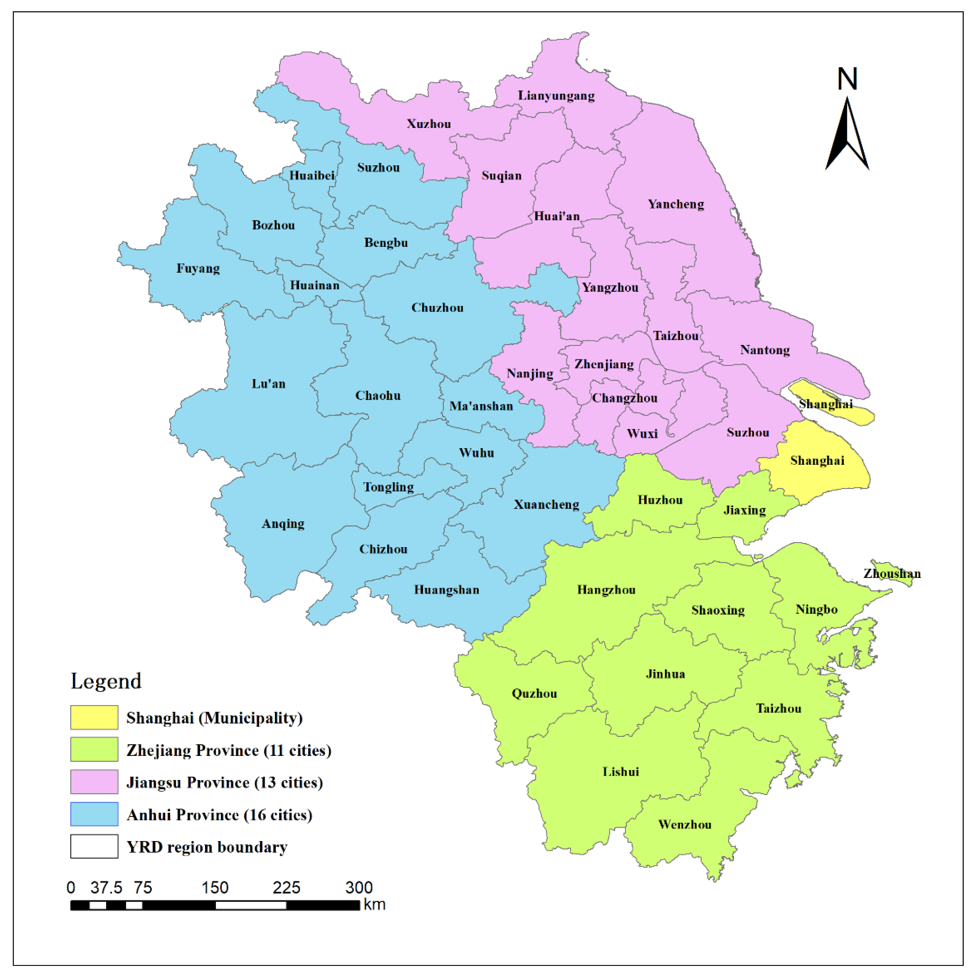
Forestry development is related to the sustainable development of China’s social economy. Forest resources are pivotal in building ecosystems and improving carbon sink capacity. The role of forest resources in sustainable economic development has attracted more attention from scholars and policymakers. Forest growth plays a very important role in climate regulation [1]. In 2017, the State Forestry Administration issued the “13th Five-Year Plan for Forestry Development” to promote the modernization of China’s forestry. In 2021, the “14th Five-Year Plan for Forestry and Grassland Protection and Development Plan” was released. By 2025, China’s forest coverage rate will be increased to 24.1%, and the forest stock volume will be increased to 19 billion m3. The Yangtze River Delta (YRD) region is the hub of China’s economic development and has an important strategic position in the overall regional development pattern. In June 2016, the “Yangtze River Delta Urban Agglomeration Development Plan” was promulgated. Boosting the construction of a green and low-carbon ecological city has become one of the important goals of the integrated development of the YRD. In 2018, the integrated development of the YRD was officially elevated to a national strategy. From 2000 to 2018, the forest coverage rate in the YRD region increased from 22.29% to 29.33%, much higher than the national average. However, the distribution of forest resources is uneven, and the structure is unreasonable. During the same period, the economic development of the YRD region was higher than the national average level and showed obvious regional differences. In December 2019, an Outline of the Yangtze River Delta Regional Integrated Development Plan was issued to prioritize ecological protection and strive to build a beautiful Yangtze River Delta. In the 14th Five-Year Plan of each province and city, increasing forest coverage has become one of the common goals for all the cities in the YRD. The YRD region is a cluster of 41 cities in 1 municipality (Shanghai) and 3 Provinces (Jiangsu, Zhejiang, and Anhui) [2,3]. Figure 1 shows the location of the YRD region.
There may be a phenomenon of “tragedy of the commons” for forest resources. One of the reasons for this phenomenon is that the beneficiaries of the use of resources and services do not need to pay for it. The costs and benefits are not equal. Unfair allocation of resource property rights will affect the fairness and efficiency of resources and social benefits and may lead to resource rent-seeking and corruption [5]. The resource curse can be turned into welfare if resources are effectively managed [6].
Some scholars have studied whether the environmental Kuznets curve (EKC) exists between forest resources and economic development, but the conclusion is also controversial [7,8,9]. The EKC assumes an inverted U-shaped relationship between economic growth and environmental quality, which means a country or region’s environmental quality will decrease with economic development. Still, when the economy develops to a certain level, the environmental quality will gradually improve [9]. Therefore, this paper’s motivation is to empirically explore the impact on the economy at different stages of forest resource development in the YRD region.
This paper mainly studies the following questions: (1) Does the abundance of forest resources in the YRD promote economic development at the city (city in this paper includes urban and rural areas) level? (2) Is there any non-linear relationship between the two? (3) Is there any evidence of the spatial spillover effect? (4) Can the abundance of forest resources improve green total factor productivity? (5) Does economic development affect forest growth, and does the Environmental Kuznets Curve exist? The possible academic contributions of this paper include: (1) Based on the resource curse hypothesis, the impact of natural resources on economic development is discussed from the perspective of renewable resources. (2) Both the quantity and quality of economic development are considered. GDP per capita (although GDP is national and gross regional product (GRP) is regional, GRP is conceptually equivalent to GDP [10]. For readers to understand easily, the term “GDP” is still used in this paper instead of “GRP”) and the green total factor productivity are analyzed further to comprehensively measure the economic development level of the YRD region. (3) This paper adopts a spatial econometric model, which not only considers general economic and social factors but also takes the spatial factors into account. The research in this paper complements the existing literature and provides a reference for policymakers.
The paper is structured as follows. Section 2 presents the literature review. Section 3 presents the econometric models, data collection, and categories of the variables. In Section 4, we describe the model estimation’s main results, including direct effects, spatial spillover effects, the robustness check, and reverse causation. In Section 5 and Section 6, we discuss the results and then draw the main conclusions.

2. Literature Review

2.1. Impacts of Forest Resources on Economic Growth

There are many studies on forest resources and economic development. Whether forest resources can promote economic development is still inconclusive. Some scholars believe that abundant forest resources will promote economic development. The importance of natural capital to economic growth is increasingly recognized, and natural forest capital positively affects national economic growth [11]. Forest resources will contribute to the total economic value through direct use value, option value, existence value, negative externality, etc. [12]. The richer the forest resources, the better the forestry sector, and the more income from harvesting non-precious wood [13]. In addition, forest-rich areas can positively impact the national economy through employment and increased labor income [14]. Rents from forest resources, mineral resources, and oil extraction contribute significantly to economic growth. At the same time, it is necessary to consider the limited availability of natural resources and stimulate the economy by developing policies and utilizing the rents of natural resources to promote development of the business environment [15]. The existence of forest resources is closely related to poverty alleviation. Forest resources and tree systems maintain welfare levels mainly by helping households increase their income and provide food, health, and humanistic values [16]. Based on SWOT and AHP analysis methods, it was found that the rise and development of the Forest Recreation Industry have expanded the regional brand effect, increased income, and enhanced the competitiveness of the industry [17]. The benefits of forest tourism will benefit residents by more than 40%, but urban residents benefit more than rural residents. The infrastructure construction brought by forest resources can also optimize industrial and investment structures [18]. Rural communities that depend on forests experience population decline and economic prosperity often. Van Kooten et al. (2019) explored how communities with rich forest resources as their main economic source stimulate economic development by examining the potential of different forest management regimes to create more jobs and wealth [19].
There is a synergy between forests and sustainable development [20], and forests have a potential role in reducing carbon emissions and poverty [21,22]. There are two main modes in which forest resources can reduce poverty. First, good management patterns can improve the quality of forest resources, thereby improving local economic conditions. Second, increasing forest resources can effectively increase natural capital and ultimately produce economical capital outcomes [23]. However, a review of 242 documents found that although the evidence of forest resource-based poverty reduction is increasing, the results are biased. More comprehensive and robust evidence is also needed to demonstrate and understand differences in outcomes across social backgrounds, social groups, and management objectives [24].
Some scholars believe that abundant forest resources will inhibit economic development. Dependence on forest resources will bring about an obvious resource curse effect [25], mainly because the forestry industry is inefficient and the industrial advantages are not obvious [26]. Another important reason is the existence of the Dutch disease effect. Areas with abundant forest resources mainly rely on the export of forest products to obtain income. However, when the international trade situation is not good, the income of exporting countries will be reduced. For countries with a single source of income, the economy will be greatly affected negatively [27]. Combining the data from 1980 to 2018, using the panel vector autoregression (PVAR) method, it was found that natural resources have an inhibitory effect on economic development in African countries. Economic growth is no longer driven solely by natural resource rents [28].

2.2. Debate of Environmental Kuznets Curve

The EKC between the exploitation and utilization of forests and economic development has always been one of the unsolved problems of environmental economics. Economies make full use of their environmental resources during initial growth. However, when the economy grows beyond a certain level, the environmental recession reaches a tipping point [29]. Hao et al. (2019) tested the relationship between forest resources and economic growth based on the assumption of the EKC using panel data from 30 provinces in China from 2002 to 2015 and the GMM model. The empirical results show that if the economy continues to grow, wood production and afforestation areas will first increase and then decrease after reaching the corresponding inflection point. It proves the existence of EKC between forest resources and economic development [30]. Based on panel data and GMM measurement methods, the empirical test verifies an environmental Kuznets curve between China’s provincial-level forest coverage and GDP per capita. Forest resources are already vital to the sustainable development of the economy. The development of urbanization and industrialization has a greater impact on China’s forest ecological footprint, while abundant natural resources inhibit economic development. The interaction of urbanization and human capital can alleviate the deterioration of the environment, and human capital has a regulating effect on the sustainable development of the economy [31]. Based on the panel data of 28 provinces in China from 1996 to 2012, the GMM model and the autoregressive distributed lag (ARDL) model were used to confirm the existence of the EKC [32]. However, based on the method of spatial measurement and first-order difference, it was empirically found that there was a U-shaped relationship between the forest coverage rate and GDP per capita in Sichuan, China. Still, there is no evidence to prove the existence of EKC [33].
At the international level, EKC conclusions on forest resources also differ. Combined with the pooled regression model and empirical evidence, it is proved that there is no inverted U-shaped EKC between GDP per capita and forest area in Canada [8]. Furthermore, changes in forest resources have multiple social and economic impacts. Based on the panel data of 111 countries from 1992 to 2015, the cointegration technique was used to analyze the long-term dynamic equilibrium relationship between forest coverage, economic development, agricultural area, and rural population density. Empirical results show that EKC exists in high-income countries and countries in the later stages of forest transition but not in low- and middle-income countries [34]. In addition, many scholars have discussed the EKC of deforestation to observe the impact of deforestation on economic growth [29,35,36,37,38,39]. Among them, through the non-causal investigation of the African heterogeneous panel, it was found that the rational implementation of land policy and trade policy to organize deforestation does not drag down economic growth [38].

2.3. Management of Forest Resources

Economic development will also counteract the development of forest resources. Combining the forest resource input-output model and the forest resource metabolism network model, the forest resources are rationally integrated into the social and economic system. The empirical results show that the primary manufacturing industry consumes more direct wood, and the advanced manufacturing and service industries use wood indirectly. This helps reduce competition between forest industries and sectors. Meanwhile, it is conducive to resource allocation and coordinated development of the economy and ecology [40]. However, increased agricultural productivity and rising wages do not increase local forest cover [41]. The analysis results of the integrated ecological economic model found an N-shaped curve between forest restoration level and economic development, and the forest quality and quantity increase in middle-income countries was the smallest [42]. China’s policy interventions in the forest sector have improved environmental and ecological conditions. However, whether forest resources increase depends on issues such as land planning, land practice, and land use rights [43]. China’s economic development has driven forest transformation, and economic and population growth has increased demand for forest products and deforestation. However, the government’s forest protection program eventually increased forest cover [44].
Regarding forest resource management, China’s forest resources have been developing rapidly but still face a very serious situation. For the excessive consumption of forest resources, forest resources have always emphasized efficient management to improve the economy and the effectiveness of forest resource utilization further [32,33]. The continuous increase in forest area and density in China is due to the national afforestation plan and the promotion of forest resources by environmental development [45]. The carrying capacity of forest resources is also affected by urbanization and over-harvesting of forests, especially in Jiangsu and Anhui, where the carrying capacity of forest resources is generally overloaded. Generally, afforestation, energy conservation, and emission reduction measures reduce external pressure on forests [46] by converting forest resource flow into forest resource stock, studying how to reduce dependence on foreign forest resources, adjusting industrial structure, and ultimately improving forest resource utilization structures and efficiency [47].
The purpose of this paper is to construct a spatial econometric model based on the theoretical analysis framework of the impact of forest resource abundance on economic development, and to empirically test the impact of forest resource abundance on economic development at the city level in the YRD region. Finally, this paper puts forward countermeasures and suggestions to promote the high-quality economic development of the YRD region.

3. Methodology

3.1. Theoretical Basis

According to the theory of economic development, in the initial stage, more consideration will be given to allocating limited resources to the industrial sectors with the most productive potential, that is, the greatest linkage effect. Priority is given to developing these sectors while overcoming the bottleneck of economic development. This drives the development of other industries and sectors, and the economic development at this time is unbalanced. However, when the economy enters an advanced stage, from the perspective of industrialization and speeding up economic development, various departments and industries should maintain a certain proportional relationship and development in coordination. The economic development at this time is balanced. The ultimate goal of short-term unbalanced growth is to achieve long-term balanced development. In economic decision-making, resource protection and sustainable resources utilization must be highly valued and considered comprehensively. Improving resource utilization efficiency and economic development are inseparable. For economic development, the excessive use and development of natural resources have caused problems such as resource abuse and environmental pollution, destroying the environment on which people rely, causing further poverty, and ultimately affecting economic development.
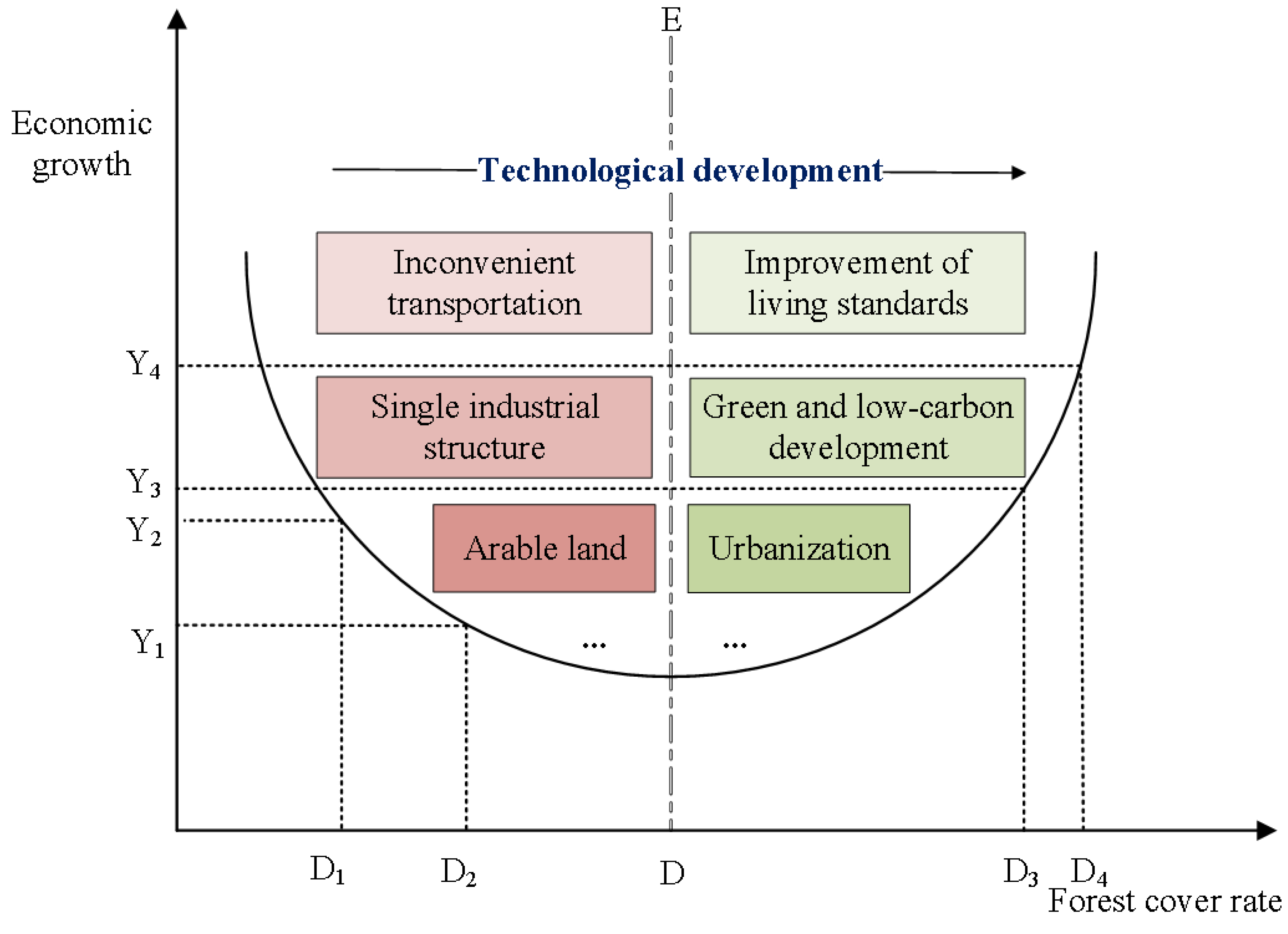
The theoretical basis of this paper is mainly analyzed from the perspective of supply and demand. In the early stage of economic development, people’s goal was survival. Transportation was inconvenient in places with abundant forest resources, and the industrial structure was single. Farmers mainly lived on cultivated land, and people had more need for basic material life. At the same time, population increase has brought enormous pressure on agricultural land, and the quality of agricultural land is getting lower and lower. This change also gradually reduces the marginal product of labor and lowers incomes [48]. Economic development is inhibited. But with the economic development to a certain extent, the rapid development of industrialization and urbanization has provided many non-agricultural employment opportunities and higher wages [49]. People’s lives have improved, and they have begun to pursue a better living environment. The economy has begun to seek green and low-carbon development. A place with abundant forest resources can promote high-quality economic development. The continuous development of science and technology makes the sustainable management of forest resources more efficient. In addition, the public health and environmental functions brought by forest resources also generates corresponding economic value [50].
In Figure 2, in the early stage of economic development, when the forest coverage rate increases from D1 to D2, economic growth will decrease from Y2 to Y1. Forest resources will affect the allocation of land resources, which may bring about poverty and ultimately affect economic development. Forests have the potential to encroach on agricultural land, and agricultural land change is often used as a proxy for forest cover loss. The increased forest resources have brought about a single industrial structure and inconvenient transportation. Initially, people could only rely on the natural forests or land converted from them for their livelihoods [29]. However, according to the elasticity of demand theory in economics, when the economy expands, people’s income levels will increase, and economic prosperity will increase people’s demand for green resources. With the advancement of technology, people’s incomes are no longer limited to arable land. Abundant forest resources have spawned tourism, led to the gathering of people, and increased employment. Increasing green supply also meets the needs of low-carbon economic development. If the forest cover rises from D3 to D4, the level of economic development will rise from Y3 to Y4. The curve to the right of the dotted line DE reflects people’s demand for forest resources with economic development. Figure 2 reflects the impact of increasing forest resources on economic growth.
Based on the above analysis, this paper proposes four hypotheses:
Hypothesis 1:
The impact of forest resource abundance on the level of economic development in the YRD region has a U-shaped non-linear characteristic.
Hypothesis 2:
The impact of forest resource abundance on economic development has spatial spillover effects in YRD.
Hypothesis 3:
The abundance of forest resources in the YRD region promotes green total factor productivity improvement.
Hypothesis 4:
The impact of economic development on the abundance of forest resources presents an environmental Kuznets curve in YRD.

3.2. Spatial Econometric Model

Spatial econometric models usually include the spatial autoregressive model (SAR), spatial error model (SEM), and spatial Durbin model (SDM). Spatial econometric models are gradually being used to verify the relationship between environmental economics studies such as carbon dioxide emissions and economic growth and to demonstrate spatial spillover effects [51].
The steps of regression analysis in this paper are as follows. First, determine whether there is a spatial correlation, and then determine whether a spatial measurement model is available. On the premise of determining the available spatial econometric model, the POLS regression is firstly performed, and the Lagrange multiplier (LM) test of the SAR and SEM models is performed simultaneously. The LM method is applied to test the spatial interaction of the data, specifically the spatial lag and spatial error autocorrelation [52]. The LM test is based on the residuals of non-spatial models with spatial fixed effects, temporal fixed effects, and spatial and temporal double fixed effects, and obeys a chi-square distribution with 1 degree of freedom. If the results reject POLS in favor of the SAR or SEM model, SDM should be selected because SDM model includes both spatially lagged explanatory variables (WY) and spatially lagged explanatory variables (WX). The spatial lag explained variable WY represents the interaction effect between the explained variable and adjacent spatial units. The SDM model can produce better fitting results [53]. The spatial benchmark regression model is constructed as follows.
Y i t = ρ W i Y t + β X i t + θ W i X i t + μ i + ξ t + ε i t
W i Y t = j = 1 n W i j Y j t
ε i t = λ M ε t + u i t  
where Y and X denote the explained variable and explanatory variable, respectively. Wi is the ith row of the spatial weight matrix W.   μ i and ξ t represent the optional individual effect and time effect, respectively. ε represents the disturbance term. i = 1, 2, …, N. t = 1, 2 …, T. W represents the spatial weighting matrix of the dependent variable, and M is the disturbance term. Wij represents the spatial weight matrices of city i and city j. ρ is the coefficient of the spatial lag term of the explained variable. θ is the spatial autocorrelation coefficient of the explanatory variable. β and θ represent the parameter vector. β reflects the influence of explanatory variables on the explained variables. λ is the coefficient of the error term. Here are two hypotheses: H0: θ = 0; H0: θ + ρ β = 0;
If θ = 0, SDM will transform into SAR,
Y i t = ρ W i Y t + X i t β + ε i t  
If θ = ρ β , SDM will transform into SEM,
Y i t = X i t β + ε i t  
If ρ = 0, λ = 0, the model will degenerate into POLS.
All the data are normalized to minimize the absolute difference and avoid the influence of extreme values. In order to prevent the bias and endogeneity problems caused by model estimation, this paper constructs SDM, SAR, and a non-spatial panel data model, respectively.
G D P P C i t = ρ j = 1 n W i j G D P P C j t + β C O R E i t + θ j = 1 n W i j C O R E i j t + β C O N T i t + θ j = 1 n W i j C O N T i j t + μ i + ξ t + ε i t
G D P P C i t = ρ j = 1 n W i j G D P P C j t + β C O R E i t + β C O N T i t + μ i + ξ t + ε i t
G D P P C i t = β C O R E i t + β C O N T i t + μ i + ξ t + ε i t
where Equations (6)–(8) are SDM, SAR, and POLS models, respectively. GDPPC is the explained variable GDP per capita, CORE is the core explanatory variable, CONT represents the control variables, β′ and β″ are the coefficients of the variables, respectively. Other variables and symbols are consistent with the base model.

3.3. Spatial Autocorrelation

This paper constructs the spatial panel data of 41 cities in the YRD region from 2007 to 2019. It uses the spatial panel econometric analysis method to test the impact of forest resource abundance on the economic development level of the YRD region. This paper constructs geospatial weights based on latitude and longitude. The variables are re-estimated based on the spatial distances of all local points in the sample set to the target analysis point. The economic geospatial weighting matrix was not used, mainly because economic conditions change yearly. The distance between two points based on the latitude and longitude distance formula is expressed as follows. The element calculation of the spatial weight matrix is determined by three factors: spatial bandwidth, kernel function, and distance calculation formula. The spatial weight matrix is expressed as follows.
W { i } = [ W { 1 } h i 0 0 W { i } h i ]
The calculation formula is: W { i } h i = f ( D { i } h i , B a n d w i d t h ) . Where D { i } h i is the distance from all data in the sample set to the local point i. f(·) is the kernel function. Bandwidth is the spatial bandwidth. One of the commonly used functions is the Gaussian function [54]. The specific representation is as follows.
W i j = exp [ 1 2 ( d i j / b ) 2 ]
where Dij represents the distance between the centroids of region i and region j. B represents bandwidth. The formula for calculating the distance between two points based on the latitude and longitude distance formula is as follows.
D { i } h i = r e × arccos [ sin ( v i ϑ ) sin ( v { i } h ϑ ) + cos ( v i ϑ ) cos ( v { i } h ϑ ) cos ( u i ϑ u { i } h ϑ ) ]
where ϑ represents an empirical constant and ϑ = π/180.   r e represents the radius of the earth. r e = 6378.1 km .
Therefore, this paper uses the latitude and longitude data of 41 cities to generate a geospatial weight matrix calculated based on the Gaussian kernel function. According to the distance weight matrix, the first judgment is the spatial autocorrelation of the explained variables. Table 1 provides Moran’s Index and Geary’s C value of the explained variables from 2007 to 2019. The Moran indices were all significantly greater than 0 and significant at the 1% level. Geary’s C is less than 1, proving a positive spatial autocorrelation relationship.

3.4. Data Sources

This paper constructs an index system from the perspectives of resources, environment, society, economy, and system to verify the influence of the abundance of forest resources in the YRD on economic development (More details in Table 2). The indicators that involve price, such as GDP, per capita consumption level, etc., are deducted from the impact of price.
The raw data are from 2005–2019. Some missing data were filled up by interpolation. There are two main methods for dealing with missing data. One is to use the mean method, which is to take the average value of two adjacent years, such as the CONPC values of Jiaxing in 2014 and 2016; the other is to use the linear interpolation method, that is, the ARIMA imputation method. This method is mainly for the lack of forest resource coverage data in 2019. We then estimate the forest area data and divide it by the land area to calculate the forest cover rate. Missing data is less than 5%. In order to investigate the economic convergence effect and time lag effect of the research city, this paper uses the real GDP per capita data from 2005 to 2019 to generate the first-order difference lag variable of the real GDP per capita. Therefore, this paper uses the 2007–2019 data as the research sample. The descriptive statistics of the data are shown in Table 3.
This paper uses the methods of variance inflation factor (VIF) and tolerance (TOL) to verify the multicollinearity of independent variables. The larger the VIF, the more severe the multicollinearity. Serious multicollinearity exists if the VIF is larger than 10. Tolerance is the inverse of VIF. A collinearity problem exists if TOL is less than 0.1. The VIF of the variables selected in this paper are below 5, and the average is 1.99 (Please see Table 4). In addition, the TOL of each indicator is above 0.1, indicating no multicollinearity.

4. Results

4.1. Direct Effects

Table 5 shows the forest resource abundance has a U-shaped non-linear effect on regional economic development. The impact of forest resource abundance on the level of economic development is negative and significant at the 10% level. Still, the relationship between the square of forest coverage and per capita GDP is positive and significant at the 1% level. It shows that in the initial stage of economic development, the abundance of forest resources negatively impacts economic growth. The main reason is that in the early stage of economic development, cities with rich forest resources often have inconvenient transportation and a single industry. The more abundant forest resources, the greater the impact on transportation and arable land. Therefore, the abundance of forest resources will inhibit economic development. However, when the economy develops to a certain extent, abundant forest resources can promote economic level improvement. This is mainly because with technology advancement, improving living standards, and people’s changing ideologies, developing the advanced service industry will be faster. Forest resources can provide better spiritual, cultural, and related products and services and improve the ecological environment. The impact of forest resources on economic development mainly includes direct, indirect, and induced effects. The direct effect is reflected in the jobs created by the forest sector, which produces indirect and induced economic added value in other sectors [14].
The first-order lag term of the explained variable is significantly negative, indicating that the phenomenon of economic convergence exists in the YRD region. If the initial state of the economy is relatively underdeveloped, there will be more room for improvement in economic development [55]. This aspect is particularly evident in Anhui Province, which is relatively underdeveloped in the YRD region. Moreover, with the Nanjing metropolitan area’s development strategy, Anhui’s economic development is relatively fast.
In terms of carbon sequestration, the impact of carbon sequestration per GDP on the level of economic development is negative and significant. Moreover, carbon sequestration has a certain social cost [56]. Economic development needs to consume a lot of resources and energy, and the production process will cause more carbon dioxide emissions. However, carbon dioxide can be absorbed through carbon sinks such as vegetation and land. The more carbon emissions, the more pollution it brings, which may ultimately inhibit regional economic development. Especially in the Anhui area, it is necessary to do a good job in the strategic layout of the low-carbon economy and circular economy development while undertaking the industrial transfer. In addition, in terms of carbon sequestration methods, there are generally two ways to increase carbon sequestration, one is by technology, and the other is by afforestation. Presently, carbon sequestration through scientific and technological means is costly. However, carbon sequestration through afforestation is currently the most economical and reliable method. Notwithstanding, large-scale afforestation may generate a lot of opportunity costs, such as land use and forestry industry development.
In terms of resources and the environment, the impact of industrial sulfur dioxide emissions per GDP on the level of economic development is positive, but the results are not significant. In addition, the impact of water resource carrying capacity on the level of economic development is negative. The more developed the economic level is, the greater the demand for resources will be and the weaker the resource-carrying capacity will be.
The impact of electricity consumption per GDP on economic development is significantly negative. Electricity consumption can reflect the economic development level of a region. However, electricity consumption and industrial structure are closely related. Generally, the demand for electricity consumption in primary and tertiary industries is not as large as that of the secondary industry. Although Jiangsu is a large manufacturing province, other industries such as finance, technology, and services are also very developed. In 2020, Shanghai’s GDP ranked among the top ten in the country, although Shanghai’s economy is relatively developed. Electricity consumption in Shanghai ranks low due to the developed tertiary industry, especially the financial industry. Industrial structure often determines electricity use, but high-tech industries typically generate much more GDP with less energy than low-end manufacturing. Especially after the implementation of power integration development, cities in the YRD gradually developed a mode of sharing and interoperability. The efficiency of energy utilization in economic development is getting higher and higher.
The YRD region is committed to industrial restructuring, optimization, and upgrading. The industry shows a trend of cluster development and can realize the integrated development of modern service and advanced manufacturing industries.
The impact of urbanization on economic development is significantly positive. Improving the urbanization level will help to improve the level of economic development. Urbanization is essentially a process of agglomeration of manpower, capital, and resources. It is also one of the important driving forces for upgrading and transforming the economic structure. The first step is the transformation of the population; that is, the rural population is transformed into an urban population and participates in non-agricultural production activities. The spatial transformation of the population residence was gradually realized after the population transformation. The transfer of rural surplus labor and the construction of cities and towns will gradually promote the development of local enterprises, thereby promoting the continuous improvement of the local economy. However, the way that accompanies economic growth is often extensive. With the continuous improvement of urbanization, higher requirements are put forward on land, culture, society, and other aspects. Ultimately, urbanization will gradually achieve coordinated development with the economy, and economic growth will gradually transit from an extensive development model to an intensive growth model.
Investment in scientific research and education has an obvious role in promoting economic development, and the estimated coefficient of the model is above 0.2. It shows that scientific and technological innovation is very important to realize the economic development of the YRD region.
Government intervention has suppressed the economic development in YRD, but the results are not significant. China’s economy has adopted a “government-led market economy” for a long time. The government intervenes deeply in the process of regional economic growth. It suppresses the role of the regional market mechanism, which may lead to imbalances in the economic structure and cannot be adjusted in time. In addition, government intervention may also bring about mistakes in decision-making and improper resources allocation. This will make the economic micro-subjects lose the initiative and vitality of economic activities. Moreover, excessive government intervention can easily lead to rent-seeking. Under modern economic conditions, the government’s main role should carry out reasonable macro-intervention and moderate guidance on economic activities through laws and regulations. However, excessive intervention may inhibit economic development.
Foreign direct investment positively impacts economic development. The more foreign direct investment, the higher the level of economic development. First, foreign investment has brought about the application and promotion of advanced green technologies and improved the production efficiency of enterprises. Second, foreign investment will also relatively impact the overall corporate environment positively through production scale expansion, industrial structure adjustment, and talent introduction. Third, by absorbing FDI, the YRD region can accelerate the accumulation of regional capital, accelerate capital formation, and further improve investment level. Meanwhile, it can promote the level of employment in the region.
In terms of consumption, the model results show that the per capita total retail sales of consumer goods positively impact economic development. The average retail sales of social consumption are generally affected by income level, price level, and consumption environment. Only with economic development, continuous improvement of residents’ income level, stable price level, and the good consumption environment can the growth of total retail sales of social consumer goods be stimulated. Conversely, the growth of consumer demand will also play a direct and final decisive role in economic growth. Investment demand and aggregate demand depend on consumption demand to some extent. From a medium and long-term perspective, only investment supported by consumer demand is effective, and effective investment and consumption make a greater contribution to economic growth.

4.2. Effects of Decomposition

The effects of spatial econometric models can be divided into direct effects, indirect effects (spatial effects), total effects, and feedback effects. The direct effect is the impact of an independent variable in a certain region on the dependent variable. The feedback effect is the direct effect coefficient minus the regression coefficient of the estimated result. The feedback effect means that the explanatory variables in a certain area will impact the explained variables in the surrounding area, which will affect the explained variables in the local area. Indirect effects are the effects of an explanatory variable on other regions, which is the influence of an explanatory variable in a neighboring area on the explained variable in the local area. The total effect is the sum of the direct and indirect effects.
Table 6 is calculated according to the spatial Durbin model of GDP per capita as the explained variable. The results show that the magnitude and significance of the coefficients of the direct effect are almost consistent with the coefficients and significance of the model estimates. The relationship between forest resource abundance and economic growth always maintains a U-shaped non-linear relationship. Forest resources can inhibit the initial stage of economic development. However, when the economy develops to a certain level, the abundance of forest resources and economic growth will develop together. Moreover, it has a positive pulling effect on the economic development of the YRD region.
Table 6 shows that the spatial effect exists. The impact of the abundance of forest resources in neighboring cities on the region’s economic development presents a non-linear inverted U-shaped trend. In the initial state, the more abundant forest resources are in neighboring cities, the more the level of economic development in the region will be promoted. When it reaches a certain level, the excessively abundant forest resources in neighboring regions will inhibit the level of economic development in the region. One reason is that the growth of trees requires material conditions such as land. Efforts to massively increase vegetation cover are increasing to alleviate climate conditions and achieve the grand vision of carbon neutrality. Excessive expansion of forest areas may seriously damage biodiversity. Cutting down old forests and planting new ones may break the original ecological balance. This will eventually crowd out the production and living resources of the region and affect economic development.
From the perspective of the feedback effect, the relationship between the abundance of forest resources of the surrounding areas and the region’s economic development again shows a non-linear U-shaped trend. It means that the direct consumption of forest resources has different impacts at different stages of economic development. With the continuous economic improvement, the sustainable development of forest resources has gradually been paid attention to. The ecological, economic, and social values of the forest have been continuously excavated. For example, after the Three Plenary Sessions of the Eleventh Session, Zhejiang entered a period of revitalization and restoration of forestry, which has been vigorously developed. While striving to develop the economy, efforts should be made to realize the sustainable utilization of forest resources. The YRD region gradually realizes the coordinated development of the environment and economy and finally promotes the sustainable development of the economy.
4.3. Robustness Check

4.3.1. Replacing the Spatial Weight Matrix

This paper adopts the spatial weight matrix of queen contiguity to verify the robustness of the estimation results. If there is a common boundary or a common contact point between two places, these two places are considered adjacent. Then we set the weight 1, otherwise 0 [57]. When performing the spatial measurement, this paper performs row normalization on the adjacent spatial weight matrix, that is, divides each element in the matrix (denoted as w i j ˜ ) by the sum of the elements in its row to ensure the sum of the elements in each row is 1, that is, w i j = w i j ˜ / j w i j ˜ . Row normalization yields the average of each region’s neighbors. In order to verify the true spatial autocorrelation relationship, the GDP per capita of the explained variable is selected to calculate Moran’s index. The significance is tested by the Monte Carlo simulation method. Moran’s index is greater than 0, and the Z value is greater than 1.96. After performing up to 99,999 permutations, the p value is always close to 0, indicating the existence of spatial autocorrelation.
After the spatial autocorrelation relationship is verified, the adjacent spatial weight matrix is used to construct a spatial econometric model. In this paper, SDM, SAR, and POLS models are set as follows:
G D P P C i t = ρ j = 1 n W i j G D P P C j t + β C O R E i t + θ j = 1 n W i j C O R E i j t + β C O N T i t + θ j = 1 n W i j C O N T i j t + μ i + ξ t + ε i t
G D P P C i t = ρ j = 1 n W i j G D P P C j t + β C O R E i t + β C O N T i t + μ i + ξ t + ε i t
G D P P C i t = β C O R E i t + β C O N T i t + μ i + ξ t + ε i t
where Equations (12)–(14) are the SDM, SAR, and POLS models, respectively. The explained variable GDP per capita, core explanatory variables, control variables, and other variables are consistent with the base model, but W i j   is replaced by the queen contiguity weighting matrix and normalized. The model results are shown in Table 7.

4.3.2. Adjusted Sample Period

In 2018, President Xi Jinping announced the integrated development of the YRD region and raised it as a national strategy. From a regional perspective, the integrated development of the YRD solves the problem of unbalanced regional development, and the integration of the YRD can play a guiding and exemplary role. Shanghai, Jiangsu, and Zhejiang are all developed regions, while Anhui is underdeveloped. The integration of the YRD needs to drive the neighboring regions with poor conditions through the regions with good conditions so that the elements flow and gather in Anhui. The YRD region should strengthen cooperation in infrastructure construction, technological innovation, industrial development, and ecological environment construction to achieve collaborative innovation and development. Therefore, the article adopts the method of reducing the sample period to avoid the impact of the policy, that is, to exclude data from 2018 and 2019. The model sample period focuses on 2007–2017, and other explained variables, explanatory variables, and control variables remain unchanged. The article also reports the results of the SAR and SDM models to reduce the bias of the model results. The results are shown in Table 8.

4.3.3. Replace the Dependent Variable

In 2017, President Xi Jinping proposed five development goals of “innovation, coordination, greenness, openness, and contribution” while considering economic development, achieving resource conservation, and environmental protection. This paper adopts the method of replacing the explained variables to verify further the impact of forest resource abundance on economic development. This section replaces GDP per capita with green total factor productivity (GTFP), which is essentially one of the ways to measure green economic growth [58]. Meanwhile, to examine the linear and non-linear effects of forest resource abundance on green total factor productivity, the core explanatory variable CORE first considers the forest coverage rate FT alone. It then simultaneously considers the forest coverage rate FT and its square. In order to stabilize the results and alleviate the endogeneity problem, the static and dynamic SAR and SDM are constructed as follows. The results are shown in Table 8.
G T F P i t = ρ j = 1 n W i j G T F P j t + β C O R E i t + β C O N T i t + θ j = 1 n W i j C O N T i j t + μ i + ξ t + ε i t
G T F P i t = ρ j = 1 n W i j G T F P j t + β C O R E i t + θ j = 1 n W i j C O R E i j t + β C O N T i t + θ j = 1 n W i j C O N T i j t + μ i + ξ t + ε i t
G T F P i t = τ G T F P i , t 1 + ρ j = 1 n W i j G T F P j , t 1 + ρ j = 1 n W i j G T F P j t + β C O R E i t + θ j = 1 n W i j C O R E i j t + β C O N T i t + θ j = 1 n W i j C O N T i j t + μ i + ξ t + ε i t
where Equations (15)–(17) represent the static SAR, the static SDM, and the dynamic SDM, respectively. The explained variable GTFP is green total factor productivity. The core explanatory variables, control variables, other variables, and symbols are consistent with the benchmark model, and the spatial weight matrix adopts the Gaussian kernel function distance weight matrix.
As shown in Table 7 and Table 8, the signs of all variables are basically unchanged. The phenomenon of economic convergence exists at the city level in the YRD region, and there is a lot of room for improvement in areas with relatively backward economies. The impact of forest resource abundance on the level of economic development has always maintained a U-shaped trend. Forest resources at the urban level in the YRD will play different roles in different stages of economic development, especially under the goal of low-carbon economic development. Resources play a pivotal role in carbon sequestration. This proves that the results of the model argument are robust. After the optimization and upgrading of the industrial structure, the energy utilization rate is high, and the investment in urbanization and science and technology education can effectively promote the economic level of the YRD region.
Table 9 shows the results of the influence of forest resource abundance on the green total factor productivity. SAR (1) and SAR (2) examine the linear and non-linear relationship between the abundance of forest resources and the level of green economic development. SDM (1) and SDM (2) represent the static and dynamic models, respectively. The results of the models show inertia in developing a green economy in the YRD region. The U-shaped characteristics of the impact of forest resource abundance on green economic development have not been verified. However, the impact of forest resource abundance on the development of the green economy is always positive. It shows that increasing the abundance of forest resources in the YRD will help improve its green economic development level and contribute to sustainable economic development. Greening is conducive to solving the trade-off dilemma of “economic growth, environmental friendliness, and resource conservation” in economic development. This is also in line with China’s current “14th Five-Year Plan” and the strategic need for sustainable economic development. All results prove that the influence of forest resource abundance on economic development in the YRD region presents a U-shaped feature, and forest resource abundance is conducive to improving green total factor productivity.

4.4. Reverse Causation

In order to verify the impact of economic development on forest resource abundance, this paper constructs the dynamic SDM model, where the dependent variable is the Forest Resource Abundance (FT), and the core explanatory variables are the economic development, namely GDP per capita (GDPPC) and its square to adopt the environmental Kuznets curve. Other control variables are kept consistent with the baseline model. The spatial weight matrix adopts the queen adjacent weight matrix. Furthermore, this paper also examines the linear relationship between economic development and forest resource abundance. All variables are standardized. The estimation results of the SAR model are also shown to check the robustness of the results.
As shown in Table 10, although there is a U-shaped curve between the level of economic development and the abundance of forest resources, the results are not stable. However, the level of economic development inhibits the abundance of forest resources. There are two main reasons. First, the cost of land-use is high in YRD. This region contributes a lot to the national economy and is one of the important urban agglomerations in China. The total economic volume accounts for 25% of the country’s total. In addition, the two most powerful harbors in the world, Shanghai and Zhoushan, are located here. Among the top 20 cities in terms of GDP, cities in the YRD region account for one-third at least. However, the area of such an economically developed region is only 358,000 km2, accounting for about 4% of the country’s total. Second, forest resources are limited by land and depend largely on territorial planning, which is difficult to change in the short term. The growth of forest resources has always been a key concern of forestry. However, from the perspective of economic development and forest land use, large, continuous forests have the potential to be transformed into smaller, isolated fragmentation processes, which exacerbate the degree of forest fragmentation [59].

5. Discussions

This paper mainly uses the method of spatial econometrics, based on the data of 41 cities in the YRD region from 2007 to 2019, to analyze the influence and spatial effects of the abundance of forest resources in the YRD region on the level of economic development. The robustness check of the results is carried out by changing the spatial weight matrix, adjusting the sample period, and changing the explained variables. The results of the model estimates are proven to be robust. The main results about our hypotheses are as follows.
Hypothesis 1 was verified. The influence of the abundance of forest resources on the economic development level in the YRD has a U-shaped non-linear characteristic [60]. At the city level in the YRD, forest resources will play different roles in different stages of economic development. The curse of forest resources will gradually evolve into welfare with economic development. In the initial stage of economic development, the abundance of forest resources has a certain inhibitory effect on the level of economic development. When the economy develops to a certain level, abundant forest resources can promote the level of economic development [15].
Hypothesis 2 was verified. Spatial spillover effects of forest resources exist [61]. Spatial factors play an important role in economic growth and convergence. The spatial autocorrelation relationship of economic development level exists. Ignoring spatial factors may lead to biased estimation results. The spatial effects of forest resource abundance on local and surrounding areas are non-linear. However, when we implement the policy of increasing forests and reducing carbon emissions, it must be within a reasonable range. Excessive forest resources may have social costs [56]. It may eventually crowd out the production and living resources of the region and affect economic development.
Hypothesis 3 was verified. The abundance of forest resources can also promote the development of green total factor productivity. This aligns with the great vision of carbon peaking and carbon neutrality. In the long run, the abundance of forest resources will help improve the quantity and quality of economic development, which is consistent with the strategic goals of China’s “14th Five-Year Plan” [62].
Hypothesis 4 was not verified. The impact of economic development on the abundance of forest resources does not show any evidence of an EKC curve in the YRD region. Furthermore, the level of economic development inhibits the forest growth. This is mainly due to the expensive land cost in the YRD region and the government’s land-use planning. Generally, competing land-use values can lead to changes in land use, which in turn affect increases or decreases in forest cover [63]. In addition, economic and population growth will increase the demand for forest products and may reduce forest resources [44].

6. Conclusions

Based on the theoretical basis of the resource curse and economic growth, this article attempts to verify the impact of urban forest resource abundance on economic development in the YRD region from the perspective of renewable resources. The research results of this paper provide a reference for the coordinated development of resources and the economy.
The influence of forest resource abundance on economic development in YRD region presents a U-shaped non-linear relationship, and the phenomenon of the resource curse will evolve into resource welfare with the development of society. In addition, the abundance of forest resources can directly promote the improvement of green total factor productivity. However, economic development may inhibit the forest growth, mainly because of the high cost of land in the YRD region. Therefore, there is only a one-way causal relationship between forest resources and economic performance, while economic performance has no feedback effect on forest resources [64].
The impact of forest resource abundance on economic development is affected by many factors, including the initial level of the economy, carbon sequestration potential, energy consumption, urbanization level, science and technology, education level, and other factors. All act together on economic growth.
Although forest resources play a very important role in the critical period of economic transformation and development, we cannot achieve green growth and carbon reduction at the expense of economic development. Economic development and urbanization can go hand in hand with forest development but requires sound management models and additional measures [65].
The YRD region should further adjust and optimize their industrial structure. Each region should implement the industrial dislocation development strategy according to its advantages, give full play to the agglomeration effect and scale effect, and realize the integrated development of modern service and advanced manufacturing industries. Much more attention should be paid to the agglomeration of high-quality talents, capital, and resources. Urbanization is still regarded as a driving force for the upgrading and transformation of the economic structure. Urbanization should gradually realize coordinated development with the economy and gradually transform the extensive development mode into the intensive economic growth mode. In addition, technological innovation is very important to realize the economic development of the YRD region. Especially in the era of the digital economy, increasing investment in scientific research can effectively improve the level of economic development [66]. Meanwhile, the government should moderately intervene in economic development.
However, the article does have certain flaws. For example, the measure of forest resource abundance is relatively simple on how to manage forest resources efficiently. This is mainly due to the lack of statistical data and methods of forest resources and technology. In future research, forest resources should be refined and classified to analyze better the impact of forest resource abundance on the economy and specific paths and then provide useful suggestions for policymakers.

Author Contributions

Conceptualization, Q.Z.; methodology, Q.Z.; formal analysis, Q.Z.; investigation, D.T.; data curation, Q.Z.; writing—original draft preparation, Q.Z.; writing—review and editing, V.B. and D.T.; visualization, Q.Z.; supervision, D.T.; All authors have read and agreed to the published version of the manuscript.

Funding

This study was funded by the National Social Science Foundation of China (Grant No. 21BJY085) and the Soft Science Project of Jiangsu Provincial Department of Science and Technology (Grant No. BR2021003).

Data Availability Statement

The data presented in this study are available on request from the corresponding author. The data are not publicly available due to other unpublished articles.

Conflicts of Interest

The authors declare no conflict of interest.

References

  1. Wang, J.; Feng, L.; Palmer, P.I.; Liu, Y.; Fang, S.; Bösch, H.; O’Dell, C.W.; Tang, X.; Yang, D.; Liu, L.; et al. Large Chinese land carbon sink estimated from atmospheric carbon dioxide data. Nature 2020, 586, 720–723. [Google Scholar] [CrossRef]
  2. Wu, X.; Tian, Z.; Kuai, Y.; Song, S.; Marson, S.M. Study on spatial correlation of air pollution and control effect of development plan for the city cluster in the Yangtze River Delta. Socioecon. Plann. Sci. 2021, 83, 101213. [Google Scholar] [CrossRef]
  3. Xia, C.; Zheng, H.; Meng, J.; Li, S.; Du, P.; Shan, Y. The evolution of carbon footprint in the yangtze river delta city cluster during economic transition 2012-2015. Resour. Conserv. Recycl. 2022, 181, 106266. [Google Scholar]
  4. Zhang, Y.; Cao, W.; Zhang, K. Mapping Urban Networks through Inter-Firm Linkages: The Case of Listed Companies in Yangtze River Delta, China. J. Geosci. Environ. Prot. 2020, 08, 23–36. [Google Scholar] [CrossRef]
  5. Angrist, J.D.; Kugler, A.D. Rural windfall or a new resource curse? coca, income, and civil conflict in Colombia. Rev. Econ. Stat. 2008, 90, 191–215. [Google Scholar] [CrossRef]
  6. Dauvin, M.; Guerreiro, D. The Paradox of Plenty: A Meta-Analysis. World Dev. 2017, 94, 212–231. [Google Scholar] [CrossRef]
  7. Mather, A.S.; Needle, C.L.; Fairbairn, J. Environmental Kuznets Curves and Forest Trends. Geography 1999, 84, 55–65. [Google Scholar]
  8. Lantz, V. Is there an Environmental Kuznets Curve for clearcutting in Canadian forests? J. For. Econ. 2002, 8, 199–212. [Google Scholar] [CrossRef]
  9. Mbatu, R.S.; Otiso, K.M. Chinese economic expansionism in Africa: A theoretical analysis of the environmental Kuznets Curve Hypothesis in the Forest Sector in Cameroon. African Geogr. Rev. 2012, 31, 142–162. [Google Scholar] [CrossRef]
  10. Viet, V.Q. Gross regional product (GRP): An introduction. United Nations Stat. Div. Retrieved August 2010, 15–17. Available online: https://unstats.un.org/unsd/economic_stat/China/background_paper_on_GRP.pdf (accessed on 30 August 2022).
  11. Naidoo, R. Economic growth and liquidation of natural capital: The case of forest clearance. Land Econ. 2004, 80, 194–208. [Google Scholar] [CrossRef]
  12. Pak, M.; Türker, M.F.; Öztürk, A. Total economic value of forest resources in Turkey. African J. Agric. Res. 2010, 5, 1908–1916. [Google Scholar] [CrossRef]
  13. Damette, O.; Delacote, P. The Environmental Resource Curse Hypothesis: The Forest Case. INRA Lab. d’Economie For. 2009, 4, hal-01189378. [Google Scholar] [CrossRef]
  14. Li, Y.; Mei, B.; Linhares-Juvenal, T. The economic contribution of the world’s forest sector. For. Policy Econ. 2019, 100, 236–253. [Google Scholar] [CrossRef]
  15. Huang, Y.; Raza, S.M.F.; Hanif, I.; Alharthi, M.; Abbas, Q.; Zain-ul-Abidin, S. The role of forest resources, mineral resources, and oil extraction in economic progress of developing Asian economies. Resour. Policy 2020, 69, 101878. [Google Scholar] [CrossRef]
  16. Hogarth, N.J.; Belcher, B.; Campbell, B.; Stacey, N. The Role of Forest-Related Income in Household Economies and Rural Livelihoods in the Border-Region of Southern China. World Dev. 2013, 43, 111–123. [Google Scholar] [CrossRef]
  17. Lu, J.; Li, M. Research on the Development of Forest Recreation Industry Based on SWOT and AHP Model-Take the Forest Recreation Industry of Xiying Street in Jinan City as an Example. IOP Conf. Ser. Earth Environ. Sci. 2022, 966. [Google Scholar] [CrossRef]
  18. Song, M.; Xie, Q.; Tan, K.H.; Wang, J. A fair distribution and transfer mechanism of forest tourism benefits in China. China Econ. Rev. 2020, 63, 101542. [Google Scholar] [CrossRef]
  19. van Kooten, G.C.; Nijnik, M.; Bradford, K. Can carbon accounting promote economic development in forest-dependent, indigenous communities? For. Policy Econ. 2019, 100, 68–74. [Google Scholar] [CrossRef]
  20. Zhang, Y.; Zhang, T.; Zeng, Y.; Cheng, B.; Li, H. Designating National Forest Cities in China: Does the policy improve the urban living environment? For. Policy Econ. 2021, 125, 102400. [Google Scholar] [CrossRef]
  21. Swamy, L.; Drazen, E.; Johnson, W.R.; Bukoski, J.J. The future of tropical forests under the United Nations Sustainable Development Goals. J. Sustain. For. 2018, 37, 221–256. [Google Scholar] [CrossRef]
  22. Zhang, Y.; Chen, J.; Han, Y.; Qian, M.; Guo, X.; Chen, R.; Xu, D.; Chen, Y. The contribution of Fintech to sustainable development in the digital age: Ant forest and land restoration in China. Land use policy 2021, 103, 1–9. [Google Scholar] [CrossRef]
  23. Miller, D.C.; Rana, P.; Nakamura, K.; Irwin, S.; Cheng, S.H.; Ahlroth, S.; Perge, E. A global review of the impact of forest property rights interventions on poverty. Glob. Environ. Chang. 2021, 66, 102218. [Google Scholar] [CrossRef]
  24. Cheng, S.H.; MacLeod, K.; Ahlroth, S.; Onder, S.; Perge, E.; Shyamsundar, P.; Rana, P.; Garside, R.; Kristjanson, P.; McKinnon, M.C.; et al. A systematic map of evidence on the contribution of forests to poverty alleviation. Environ. Evid. 2019, 8, 1–22. [Google Scholar] [CrossRef]
  25. Zhang, Q.; Brouwer, R. Is China Affected by the Resource Curse? A Critical Review of the Chinese Literature. J. Policy Model. 2020, 42, 133–152. [Google Scholar] [CrossRef]
  26. Liu, Z.; Yao, S.; Liu, Y. Forest resource curse based on spatial panel modeling. Resour. Sci. 2015, 37, 379–390. [Google Scholar]
  27. Gibson, J. Forest Loss and Economic Inequality in the Solomon Islands: Using Small-Area Estimation to Link Environmental Change to Welfare Outcomes. Ecol. Econ. 2018, 148, 66–76. [Google Scholar] [CrossRef]
  28. Aslan, A.; Altinoz, B. The impact of natural resources and gross capital formation on economic growth in the context of globalization: Evidence from developing countries on the continent of Europe, Asia, Africa, and America. Environ. Sci. Pollut. Res. 2021, 28, 33794–33805. [Google Scholar] [CrossRef]
  29. Caravaggio, N. Economic growth and the forest development path: A theoretical re-assessment of the environmental Kuznets curve for deforestation. For. Policy Econ. 2020, 118, 102259. [Google Scholar] [CrossRef]
  30. Hao, Y.; Xu, Y.; Zhang, J.; Hu, X. Relationship between forest resources and economic growth: Empirical evidence from China. J. Clean. Prod. 2019, 214, 848–859. [Google Scholar]
  31. Ahmed, Z.; Asghar, M.M.; Malik, M.N.; Nawaz, K. Moving towards a sustainable environment: The dynamic linkage between natural resources, human capital, urbanization, economic growth, and ecological footprint in China. Resour. Policy 2020, 67, 101677. [Google Scholar] [CrossRef]
  32. Li, T.; Wang, Y.; Zhao, D. Environmental Kuznets Curve in China: New evidence from dynamic panel analysis. Energy Policy 2016, 91, 138–147. [Google Scholar] [CrossRef]
  33. Zhao, H.; Uchida, E.; Deng, X.; Rozelle, S. Do Trees Grow with the Economy? A Spatial Analysis of the Determinants of Forest Cover Change in Sichuan, China. Environ. Resour. Econ. 2011, 50, 61–82. [Google Scholar] [CrossRef]
  34. García, V.R.; Caravaggio, N.; Gaspart, F.; Meyfroidt, P. Long-and short-run forest dynamics: An empirical assessment of forest transition, environmental kuznets curve and ecologically unequal exchange theories. Forests 2021, 12, 431. [Google Scholar] [CrossRef]
  35. Culas, R.J. Deforestation and the environmental Kuznets curve: An institutional perspective. Ecol. Econ. 2007, 61, 429–437. [Google Scholar] [CrossRef]
  36. Culas, R.J. REDD and forest transition: Tunneling through the environmental Kuznets curve. Ecol. Econ. 2012, 79, 44–51. [Google Scholar] [CrossRef]
  37. Choumert, J.; Combes Motel, P.; Dakpo, H.K. Is the Environmental Kuznets Curve for deforestation a threatened theory? A meta-analysis of the literature. Ecol. Econ. 2013, 90, 19–28. [Google Scholar] [CrossRef]
  38. Ajanaku, B.A.; Collins, A.R. Economic growth and deforestation in African countries: Is the environmental Kuznets curve hypothesis applicable? For. Policy Econ. 2021, 129, 102488. [Google Scholar] [CrossRef]
  39. Koop, G.; Tole, L. Is there an environmental Kuznets curve for deforestation? J. Dev. Econ. 1999, 58, 231–244. [Google Scholar] [CrossRef]
  40. Zhang, X.; Huang, G.; Liu, L.; Zhai, M.; Li, J. Ecological and economic analyses of the forest metabolism system: A case study of Guangdong Province, China. Ecol. Indic. 2018, 95, 131–140. [Google Scholar] [CrossRef]
  41. Foster, A.D.; Rosenzweig, M.R. Economic growth and the rise of forests. Q. J. Econ. 2003, 118, 601–637. [Google Scholar] [CrossRef]
  42. Benedek, Z.; Fertő, I. Does economic growth influence forestry trends? An environmental Kuznets curve approach based on a composite Forest Recovery Index. Ecol. Indic. 2020, 112, 106067. [Google Scholar] [CrossRef]
  43. Aguilar, F.X.; Wen, Y. Socio-economic and ecological impacts of China’s forest sector policies. For. Policy Econ. 2021, 127, 102454. [Google Scholar] [CrossRef]
  44. Zhang, K.; Song, C.; Zhang, Y.; Zhang, Q. Natural disasters and economic development drive forest dynamics and transition in China. For. Policy Econ. 2017, 76, 56–64. [Google Scholar] [CrossRef]
  45. Shi, L.; Zhao, S.; Tang, Z.; Fang, J. The changes in China’s forests: An analysis using the forest identity. PLoS ONE 2011, 6, e20778. [Google Scholar] [CrossRef]
  46. Tang, X.; Guan, X.; Lu, S.; Qin, F.; Liu, X.; Zhang, D. Examining the spatiotemporal change of forest resource carrying capacity of the Yangtze River Economic Belt in China. Environ. Sci. Pollut. Res. 2020, 27, 21213–21230. [Google Scholar] [CrossRef] [PubMed]
  47. Cheng, S.; Xu, Z.; Su, Y.; Zhen, L. Spatial and temporal flows of China’s forest resources: Development of a framework for evaluating resource efficiency. Ecol. Econ. 2010, 69, 1405–1415. [Google Scholar] [CrossRef]
  48. Cropper, M.; Griffiths, C. The interaction of population growth and environmental quality. Am. Econ. Rev. 1994, 84, 250–254. [Google Scholar]
  49. Wang, J.; Xin, L.; Wang, Y. Economic growth, government policies, and forest transition in China. Reg. Environ. Chang. 2019, 19, 1023–1033. [Google Scholar] [CrossRef]
  50. Kim, J.S.; Lee, T.J.; Hyun, S.S. Estimating the economic value of urban forest parks: Focusing on restorative experiences and environmental concerns. J. Destin. Mark. Manag. 2021, 20, 100603. [Google Scholar] [CrossRef]
  51. Meng, L.; Huang, B. Shaping the Relationship Between Economic Development and Carbon Dioxide Emissions at the Local Level: Evidence from Spatial Econometric Models. Environ. Resour. Econ. 2018, 71, 127–156. [Google Scholar] [CrossRef]
  52. Anselin, L. Spatial Econometrics: Methods and Models; Springer Science & Business Media: Dordrecht, The Netherlands, 1988; ISBN 978-90-481-8311-1. [Google Scholar]
  53. Elhorst, J.P. Spatial Econometrics From Cross-Sectional Data to Spatial Panels; Springer: New York, NY, USA, 2014; ISBN 978-3-642-40339-2. [Google Scholar]
  54. Kang, D.; Dall’erba, S. Exploring the spatially varying innovation capacity of the US counties in the framework of Griliches’ knowledge production function: A mixed GWR approach. J. Geogr. Syst. 2016, 18, 125–157. [Google Scholar] [CrossRef]
  55. Bernard, A.B.; Durlauf, S.N. Interpreting tests of the convergence hypothesis. J. Econom. 1996, 71, 161–173. [Google Scholar] [CrossRef]
  56. Castro-Magnani, M.; Sanchez-Azofeifa, A.; Metternicht, G.; Laakso, K. Integration of remote-sensing based metrics and econometric models to assess the socio-economic contributions of carbon sequestration in unmanaged tropical dry forests. Environ. Sustain. Indic. 2021, 9, 100100. [Google Scholar] [CrossRef]
  57. LeSage, J. The Theory and Practice of spatial Econometrics; Department of Economics, University of Toledo: Toledo, OH, USA, 1999. [Google Scholar]
  58. Li, J.; Xu, B. Curse or Blessing: How Does Natural Resource Abundance Affect Green Economic Growth in China? Econ. Res. J. 2018, 139, 151–167. [Google Scholar]
  59. Li, L.; Deng, D.; Zhang, D.; Yang, W. Analysis on Socio-economic Determinants of Forest Fragmentation in Beijing-Tianjin-Hebei Region. For. Econ. 2021, 04, 5–16. [Google Scholar] [CrossRef]
  60. Wang, S.; Liu, C.; Wilson, B. Is China in a later stage of a U-shaped forest resource curve? A re-examination of empirical evidence. For. Policy Econ. 2007, 10, 1–6. [Google Scholar] [CrossRef]
  61. Gong, Z.; Gu, L.; Yao, S.; Deng, Y. Effects of bio-physical, economic and ecological policy on forest transition for sustainability of resource and socioeconomics development. J. Clean. Prod. 2020, 243, 118571. [Google Scholar] [CrossRef]
  62. Lin, B.; Ge, J. Carbon sinks and output of China’s forestry sector: An ecological economic development perspective. Sci. Total Environ. 2019, 655, 1169–1180. [Google Scholar] [CrossRef] [PubMed]
  63. Barbier, E.B.; Delacote, P.; Wolfersberger, J. The economic analysis of the forest transition: A review. J. For. Econ. 2017, 27, 10–17. [Google Scholar] [CrossRef]
  64. Xie, M.; Irfan, M.; Razzaq, A.; Dagar, V. Forest and mineral volatility and economic performance: Evidence from frequency domain causality approach for global data. Resour. Policy 2022, 76, 102685. [Google Scholar] [CrossRef]
  65. Choi, Y.; Lim, C.H.; Chung, H.I.; Kim, Y.; Cho, H.J.; Hwang, J.; Kraxner, F.; Biging, G.S.; Lee, W.K.; Chon, J.; et al. Forest management can mitigate negative impacts of climate and land-use change on plant biodiversity: Insights from the Republic of Korea. J. Environ. Manage. 2021, 288, 112400. [Google Scholar] [CrossRef]
  66. Li, L.; Hao, T.; Chi, T. Evaluation on China’s forestry resources efficiency based on big data. J. Clean. Prod. 2017, 142, 513–523. [Google Scholar] [CrossRef]
Figure 1. Location of the YRD region [4]. Reproduced from [4], with permission from Scientific Research Publishing, 2020.
Forests 13 01605 g001
Figure 2. Theoretical framework.
Forests 13 01605 g002
Table 1. Moran’s I and Geary’s C based on the distance weighting matrix.
YearMoran’s IGeary’s C
IZ Valuep ValueCZ Valuep Value
20070.4314.4600.0000.547−3.7380.000
20080.4234.3820.0000.537−3.8290.000
20090.3954.1000.0000.569−3.5810.000
20100.3553.6950.0000.596−3.4380.001
20110.3884.0260.0000.581−3.5590.000
20120.4044.1850.0000.593−3.4300.001
20130.3833.9700.0000.602−3.3790.001
20140.3813.9530.0000.598−3.4020.001
20150.3894.0320.0000.589−3.4950.000
20160.4234.3670.0000.535−3.9210.000
20170.4164.2920.0000.572−3.6130.000
20180.4154.2800.0000.552−3.8100.000
20190.4014.1440.0000.568−3.6740.000
Table 2. Data source and variables.
VariableDefinitionMeasurementData source
Dependent variable
GDPPCReal GDP per capitaReal GDP divided by the total resident population of each citySYB
Core independent variable
FTForest cover rateForest area divided by land areaSYB, JFB, ZFRMC
FT2Square of forest cover rateSquare of (forest area divided by land area)SYB, JFB, ZFRMC
Control variable
L.GDPPCTime lag effect of the level of economic developmentThe first-order difference lag variable of the GDP per capitaSYB
CSGDPCarbon sequestration per GDPCarbon sequestration divided by real GDPCEADS
ISO2GDPIndustrial sulfur dioxide emissions per GDP Industrial SO2 emissions divided by GDPCNKI, CUSY, DEEA
WLIWater resources carrying capacityRatio of per capita domestic water use to total per capita water resourcesSYB, WRB
EUGDPElectricity consumption per capita per GDPThe per capita electricity consumption of the whole society divided by GDPIFIND
URBUrbanization rateUrban population of each city divided by the total permanent populationSYB, SB
SECGDPIndustrial structureThe growth value of the secondary industry as a proportion of GDPCNKI, SYB
KJScience and technology education levelProportion of education and science and technology expenditures in local budgets to total expendituresIFIND
GIGovernment interventionThe local budget expenditures deduct the remaining expenditures on education and science and technology as a percentage of GDP IFIND
FDIGDPLevel of foreign investmentThe proportion of foreign capital actually utilized by cities in GDPCNKI, SYB
CONPCConsumption per capitaThe total retail sales of consumer goods in the region divided by the resident population of the regionIFIND
Note: SYB: Statistical yearbooks of provinces and cities over the years; JFB: Jiangsu Forestry Bureau; ZFRMC: Zhejiang Forest Resources Monitoring Center; CEADS: Carbon Emission Accounts & Datasets; CNKI: Platform of China National Knowledge Infrastructure; CUSY: China Urban Statistical Yearbook; DEEA: Department of Ecology and Environment of Anhui Province; WRB: Water Resources Bulletin; IFIND: Financial Data Center; SB: Statistical Bulletins of National Economic and Social Development of All Cities.
Table 3. Descriptive statistics of variables.
VariablesObsMeanStd. Dev.MinMaxUnit
GDPPC5335.8579 3.6554 0.5515 18.0044 CNY 10,000
L.GDPPC5330.4886 0.5572 −3.7511 4.5163 CNY 10,000
FT53333.2510 20.3320 3.1700 83.2500 %
CSGDP5330.0051 0.0055 0.0002 0.0422 kg/CNY
ISO2GDP5332.7067 3.5777 0.0212 34.7532 kg/CNY
WLI5330.1069 0.1095 0.0040 1.1268 %
EUGDP5330.0877 0.0271 0.0429 0.2099 kWh/CNY
URB53358.1388 12.8491 29.0000 89.6000 %
SECGDP53348.7669 8.1090 26.9928 74.7346 %
KJ53321.0422 3.9938 1.9916 36.9996 %
GI53313.5148 5.5856 4.8154 32.1284 %
FDIGDP5333.3144 2.1926 0.2114 13.0430 %
CONPC5332.2246 1.6116 0.1881 19.4993 CNY 10,000
Table 4. Multicollinearity test of variables.
VariableVIFTOL
URB3.32 0.30
CSGDP2.56 0.39
SECGDP2.36 0.42
CONPC2.30 0.43
EUGDP2.00 0.50
WLI1.90 0.53
FT1.80 0.56
ISO2GDP1.68 0.59
GI1.68 0.59
KJ1.65 0.61
FDIGDP1.45 0.69
L.GDPPC1.170.85
Average1.990.54
Table 5. Spatial econometric estimation results.
Dependent Variable: GDP Per Capita
Spatial ModelNon-Spatial Model
VariableSARSARSDMPOLS
L.GDPPC0.0048 ***−0.0044 **−0.0051 **−0.0043 ***
(−2.8360)(−2.5635)(−2.1521)(−2.7093)
FT−0.8339 *−0.7737 *−0.9200 *−0.7556 *
(−1.9476)(−1.8489)(−1.6540)(−1.9437)
FT20.1049 ***0.1049 ***0.1142 ***0.1020 ***
(9.8163)(9.8842)(8.3547)(10.5339)
CSGDP−0.0239 *−0.0289 **−0.0421 **−0.0290 **
(−1.6717)(−1.9894)(−2.1489)(−2.1510)
ISO2GDP0.00310.00440.01600.0048
(0.3231)(0.4612)(1.2394)(0.5342)
WLI−0.0017−0.0012−0.0016−0.0011
(−0.7948)(−0.5624)(−0.5204)(−0.5702)
EUGDP−0.0564 ***−0.0541 ***−0.0585 ***−0.0524 ***
(−3.8978)(−3.6940)(−2.7759)(−3.8625)
URB0.0055 *0.0059 *0.0079 *0.0055 *
(1.6815)(1.8217)(1.7462)(1.8503)
SECGDP0.00010.00010.00010.0001
(−0.6343)(−0.4708)(−0.5026)(−0.4946)
KJ0.2607 ***0.2380 ***0.2282 *0.2256 ***
(3.1056)(2.6675)(1.7747)(2.7295)
GI−0.0081−0.0062−0.0166−0.0062
(−0.8508)(−0.6629)(−1.2419)(−0.7113)
FDIGDP0.00010.00010.00010.0001
(−0.4809)(−0.2191)(−0.1173)(−0.2292)
CONPC0.01060.01030.01090.0098
(1.4022)(1.3795)(1.0295)(1.4085)
R20.52240.59120.56960.5442
Obs533533533533
Note: *** significant at 1% level; ** significant at 5% level; * significant at 10% level; T statistic in brackets.
Table 6. Decomposition of direct effects, indirect effects, and total effects.
Dependent Variable: GDP Per Capita
Direct EffectIndirect EffectTotal EffectFeedback Effect
L.GDPPC−0.0048 ***0.0010 **−0.0039 ***0.0001
(−2.7387)(2.0410)(−2.7268)
FT−0.8623 **0.1709 *−0.6914 *−0.0284
(−2.0103)(1.6379)(−2.0121)
FT20.1062 ***−0.0209 ***0.0853 ***0.0013
(9.4994)(−3.0773)(8.9238)
CSGDP−0.0242 *0.0048−0.0195 *−0.0003
(−1.7010)(1.4741)(−1.6918)
ISO2GDP0.0039−0.00080.00310.0009
(0.4115)(−0.3999)(0.4084)
WLI−0.00170.0003−0.00130.0001
(−0.7504)(0.7133)(−0.7466)
EUGDP−0.0572 ***0.0112 **−0.0459 ***−0.0008
(−3.7210)(2.3800)(−3.6831)
URB0.0056 *−0.00110.0045 *0.0002
(1.6479)(−1.4040)(1.6441)
SECGDP0.00010.00010.00020.0001
(−0.6463)(0.6184)(−0.6423)
KJ0.2617 ***−0.0513 **0.2104 ***0.0010
(2.9847)(−2.1614)(2.9407)
GI−0.00830.0016−0.0066−0.0002
(−0.8289)(0.7771)(−0.8276)
FDIGDP0.00010.00010.00020.0001
(−0.4266)(0.4011)(−0.4267)
CONPC0.0108−0.00210.00870.0002
(1.4097)(−1.2702)(1.4002)
Note: *** significant at the 1% level; ** significant at the 5% level; * significant at the 10% level; T statistics in parentheses.
Table 7. Results of robustness check.
Dependent Variable: GDP Per Capita
VariableSARSARSDM
L.GDPPC−0.0046 *** −0.0043 ***−0.0062 ***
(−2.9053) (−2.5937)(−3.6498)
FT−0.7828 * −0.7665 * −0.6810 *
(−1.9554) (−1.8866) (−1.7427)
FT20.0991 *** 0.1016 *** 0.1013 ***
(9.8301) (9.7626) (9.2241)
CSGDP−0.0239 * −0.0286 ** −0.0289 **
(−1.7610) (−2.0085) (−1.9654)
ISO2GDP0.0031 *** 0.0047 0.0036
(0.3543) (0.5082) (0.4049)
WLI−0.0016 −0.0011 −0.0029
(−0.7919) (−0.5279)(−1.3508)
EUGDP−0.0524 *** −0.0526 *** −0.0518 ***
(−3.8967) (−3.7191) (−3.7152)
URB0.0048 0.0054 * 0.0078 **
(1.5648) (1.7179) (2.3585)
SECGDP0.0001 0.0001 0.0001
(−0.6400) (−0.4969) (−0.1923)
KJ0.2312 *** 0.2232 *** 0.1446
(2.9572) (2.5833) (1.6013)
GI−0.0076 −0.0061 −0.0075
(−0.8504) (−0.6715) (−0.8437)
FDIGDP0.0001 0.0001 0.0001
(−0.4924) (−0.2024) (0.2674)
CONPC0.0095 0.0097 0.0110
(1.3533) (1.3396) (1.5560)
R20.58540.61750.6341
Obs533533533
Note: *** significant at the 1% level; ** significant at the 5% level; * significant at the 10% level; T statistics in parentheses.
Table 8. Results of robustness checks from 2007–2017.
Dependent Variable: GDP Per Capita
Spatial ModelNon-Spatial Model
VariableSARSARSDMOLS
L.GDPPC−0.0043 *** −0.0039 ** −0.0017 −0.0042 **
(−2.6701) (−2.3535) (−0.7280) (−2.4758)
FT−0.9632 ** −0.9393 ** −0.9477 ** −0.9698 **
(−2.2326) (−2.0669) (−1.7653) (−2.0963)
FT20.0852 *** 0.0876 *** 0.0643 *** 0.0958 ***
(6.8397) (6.6826) (3.2157) (7.3667)
CSGDP−0.0197 −0.0231 0.0068 −0.0276 *
(−1.3633) (−1.5413) (0.3264) (−1.8157)
ISO2GDP0.0023 0.0034 0.0078 0.0037
(0.2929) (0.4047) (0.6696) (0.4296)
WLI−0.0021 −0.0016 0.0025 −0.0018
(−1.1307) (−0.8612)(0.9360)(−0.9445)
EUGDP−0.0432 *** −0.0429 *** −0.0367 ** −0.0447 ***
(−3.2563) (−3.0546) (−2.0033) (−3.1328)
URB0.0014 0.0027 0.0001 0.0037
(0.4392) (0.7919) (0.0020) (1.0781)
SECGDP0.0001 0.0001 0.0001 0.0001
(−0.7393) (−0.7308) (−2.5473) (−0.5204)
KJ0.2253 *** 0.2198 *** 0.0832 0.2460 ***
(2.9960) (2.7051) (0.7572) (2.9855)
GI−0.0114 −0.0127 −0.0264** −0.0137
(−1.2976) (−1.3367) (−2.0907) (−1.4166)
FDIGDP0.00010.00010.00010.0001
(−0.8932) (−0.6854) (1.5175) (−0.8663)
CONPC0.0074 0.0082 0.0162 * 0.0078
(1.0692) (1.1208) (1.7552) (1.0480)
R20.56130.59300.56180.4636
Obs451451451451
Note: *** significant at the 1% level; ** significant at the 5% level; * significant at the 10% level; T statistics in parentheses.
Table 9. Estimation results of effects of forest resource abundance on GTFP.
Dependent Variable: GTFP
VariableSAR (1)SAR (2)SDM (3)SDM (4)
L.GTFP0.4277 *** 0.4261 *** 0.4515 ***0.5420 ***
(0.0318) (0.0318) (0.0391) (0.0441)
FT0.3878 * 0.8019 ** 0.7673 *0.9644 *
(0.0381) (0.3924) (0.2998) (0.5759)
FT2 −0.6917 −0.9728
(0.5206) (0.7812)
Control variablesYesYesYesYes
R20.35270.35390.36970.4279
Obs533533533492
Note: *** significant at the 1% level; ** significant at the 5% level; * significant at the 10% level; standard errors are in parentheses.
Table 10. Estimation results of effects of economic development on forest resource abundance.
Dependent Variable: Forest Cover Rate
VariableSDM (1)SAR (2)SDM (3)SAR (4)
GDPPC−0.0680 **−0.0578 ***−0.1268 *−0.0987
(0.0277)(0.0279)(0.0749)(0.0733)
Square of GDPPC 0.03880.0271
(0.0468)(0.0459)
Control variablesYesYesYesYes
R20.99060.99050.99060.9904
Obs492492492492
Note: *** significant at the 1% level; ** significant at the 5% level; * significant at the 10% level; standard errors are in parentheses.
Publisher’s Note: MDPI stays neutral with regard to jurisdictional claims in published maps and institutional affiliations.