Efficiency Decomposition Analysis of the Marine Ship Industry Chain Based on Three-Stage Super-Efficiency SBM Model—Evidence from Chinese A-Share-Listed Companies

Abstract

Based on the micro-data of 79 listed companies in the Chinese marine ship industry chain from 2015 to 2019, this paper calculates the comprehensive technical efficiency (TE), pure technical efficiency (PTE), and scale efficiency (SE) of the upstream, midstream, and downstream of China’s marine ship industry chain by using a three-stage super-efficiency slacks-based model (SBM), and further analyzes the weak links in industrial chain efficiency and their influencing factors. It is shown that (i) the TE and PTE of the upstream, midstream, and downstream of China’s marine ship industry chain are in a “V”-shaped distribution, high at both ends and low in the middle, but that the SE is ranked as follows: upstream > midstream > downstream. In addition, the PTE is the main factor which hinders the improvement of TE in the industrial chain. (ii) The environmental variables have significant impacts on industrial chain efficiency. When the influences of environmental variables and random error terms are excluded, the industrial chain efficiency changes significantly. The values of SE and TE decrease significantly, and the distribution characteristic of TE changes. However, the PTE is still in a “V”-shaped distribution and appears to be the main driving force for the progress of TE. (iii) China’s marine ship industry chain has obvious weak links in terms of efficiency, and the midstream and downstream areas need to focus on development. Each link of the industry chain has high coupling and low coordination, and they are all closely related to each other, but the coordination ability is insufficient. The industrial chain in terms of efficiency and coordinated development can still be improved.

1. Introduction

Today, with the rapid development of international trade, marine shipping has become the main force in international trade and transportation due to its large volume and low cost [1]. With the gradual implementation of major strategic concepts, such as the 21st Century Maritime Silk Road and maritime power, marine shipping is facing ample opportunities for development. However, at the same time, many policies that aim to reduce carbon dioxide emissions from ships have also been promulgated to protect the marine environment and biodiversity. New requirements have been put forward, including green shipping and low-carbon shipping [2]. In order to achieve low-carbon shipping, it is necessary to carry out technological innovation on traditional ships, change the ships’ power systems and supporting equipment, and use more environmentally friendly materials and energy. These are the technical challenges to be faced by the shipping industry. Therefore, for marine shipping, there are both opportunities and challenges. Thus, there is the following urgent problem to be solved: how can development opportunities be seized to rapidly expand industrial strength and, at the same time, overcome technical difficulties to achieve the goal of emission reduction?

As the carriers of marine shipping, ships are the focus of implementing green shipping, low-carbon shipping, and other policies. In order to achieve the goal of reducing carbon emissions, shipbuilding companies firstly need to enhance their technological innovation capabilities, upgrade ship power systems, and use clean energy. Secondly, other shipbuilding-related companies also have to make changes. For example, marine paint manufacturers and marine supporting equipment manufacturers, such as internal combustion engine producers, also need to optimize traditional equipment to meet the requirements of carbon emission reduction. Thirdly, the use of ships with low carbon emissions will also drive enterprises relying on ships to make corresponding adjustments. These enterprises include international logistics and shipping companies, marine engineering and construction enterprises, maritime defense and military affairs enterprises, and others. The above companies are distributed throughout the ship’s entire process from construction to application. Furthermore, these companies form the marine ship industry chain, involving the upstream, midstream, and downstream of the industry chain. Therefore, it can be said that the technological upgrading of ships’ carbon emission reduction affects all links of the marine ship industry chain. The promotion of carbon reduction technologies can drive the transformation and upgrading of the whole industry chain. Therefore, grasping the status quo of industrial chain development is an important prerequisite for clarifying the impact of technological upgrading. However, until now, the research on the whole marine ship industry chain and its links has not been comprehensive enough. There is still a lack of in-depth research on whether the development of the links is balanced, efficient, and coordinated, as well as on whether there are weak links in the development of the industrial chain. Solving the above problems will play an important role in promoting the technology upgrading of ships’ carbon emission reduction. It can accelerate the pace of achieving green shipping and low-carbon shipping, and further promote the high-quality development of the marine ship industry chain.

The coordinated development of upstream, middle, and downstream enterprises in the marine ship industry chain is conducive to improving the overall operation efficiency of the industry chain [3]. This paper takes China’s ship industry chain as the empirical object, firstly because China is the largest shipbuilding country in the world. According to the world shipbuilding data released by Clarksons Research (https://sin.clarksons.net/ (accessed on 21 April 2022)), in 2020, China’s shipbuilding completion volume accounted for 43.1% of the world total, new orders accounted for 48.8% of the world total, and hand-held orders accounted for 44.7% of the world’s total. Secondly, China has a complete ship industry chain system, with rich sample data. Finally, the development process of China’s ship industry chain is tortuous. For a long time, the industry scale has developed rapidly with low-end overcapacity [4]. In particular, China’s independent innovation is weak and lacks competitiveness in the ship market. Meanwhile, the internal development of the industrial chain is unbalanced, and the ship equipment supporting capacity cannot catch up with the shipbuilding capacity [5]. The study of these problems in the development of China’s ship industry chain can provide experience for the development of other regions. By reviewing the existing literature, we found that there are few studies on the whole industry chain perspective of China’s marine ship industry chain, and most of the studies focus on the field of the shipbuilding industry [6,7,8]. However, the shipbuilding industry is only the midstream of the marine ship industry chain (the overall structure of the industrial chain is in Section 2.1). The existing literature lacks research from the perspective of the whole industry chain and lacks an investigation of the coordination degree between the upstream, midstream, and downstream of the marine ship industry chain. Moreover, the existing research mainly studies the marine ship industry chain from the macro level [9,10], and there are relatively few studies from the micro level. In view of the inadequacy of existing research, based on the data of listed companies in China’s marine ship industry chain, we conducted this research on the development level and synergy ability of each link of China’s marine ship industry chain from the micro level. The theoretical significance of this research is to enrich the research content of the marine ship industry chain from the micro level and the perspective of the whole industry chain. The practical significance is to explore the existing problems and environmental constraints in the development of China’s marine ship industry chain, as well as the unbalanced development in each link of the industry chain. After that, we further put forward targeted improvement strategies to provide the reference value for promoting the high-quality development of China’s marine ship industry chain.

Measuring the efficiency of the industrial chain is an effective way to grasp the development level of the industrial chain. There are three efficiency indicators that scholars often use, namely comprehensive technical efficiency (TE), pure technical efficiency (PTE), and scale efficiency (SE). Here, TE refers to the ratio of the minimum cost to the actual cost when an enterprise produces a certain quantity of product. The higher the TE value, the higher the production efficiency of the enterprise. On the other hand, PTE refers to the production efficiency of enterprises affected by management and technology, while SE refers to the difference between the existing scale and the optimal scale of the enterprise [11,12]. Therefore, we conducted research on the efficiency of China’s marine ship industry chain. We used the three-stage super-efficiency slacks-based model (SBM) to calculate the three efficiency values for each link and the whole industrial chain. This model uses the super-efficiency SBM model to calculate efficiency value in the first and third stages, and then uses the stochastic frontier analysis (SFA) model to remove the impact of external environmental factors on efficiency in the second stage. By measuring efficiency and exploring the mechanism of external policies affecting the overall efficiency of the industrial chain, we aim to provide policy references for effectively promoting the transformation and upgrading of the marine ship industry chain, promoting ships’ carbon emission reduction, and engaging in green shipping.

2. Literature Review

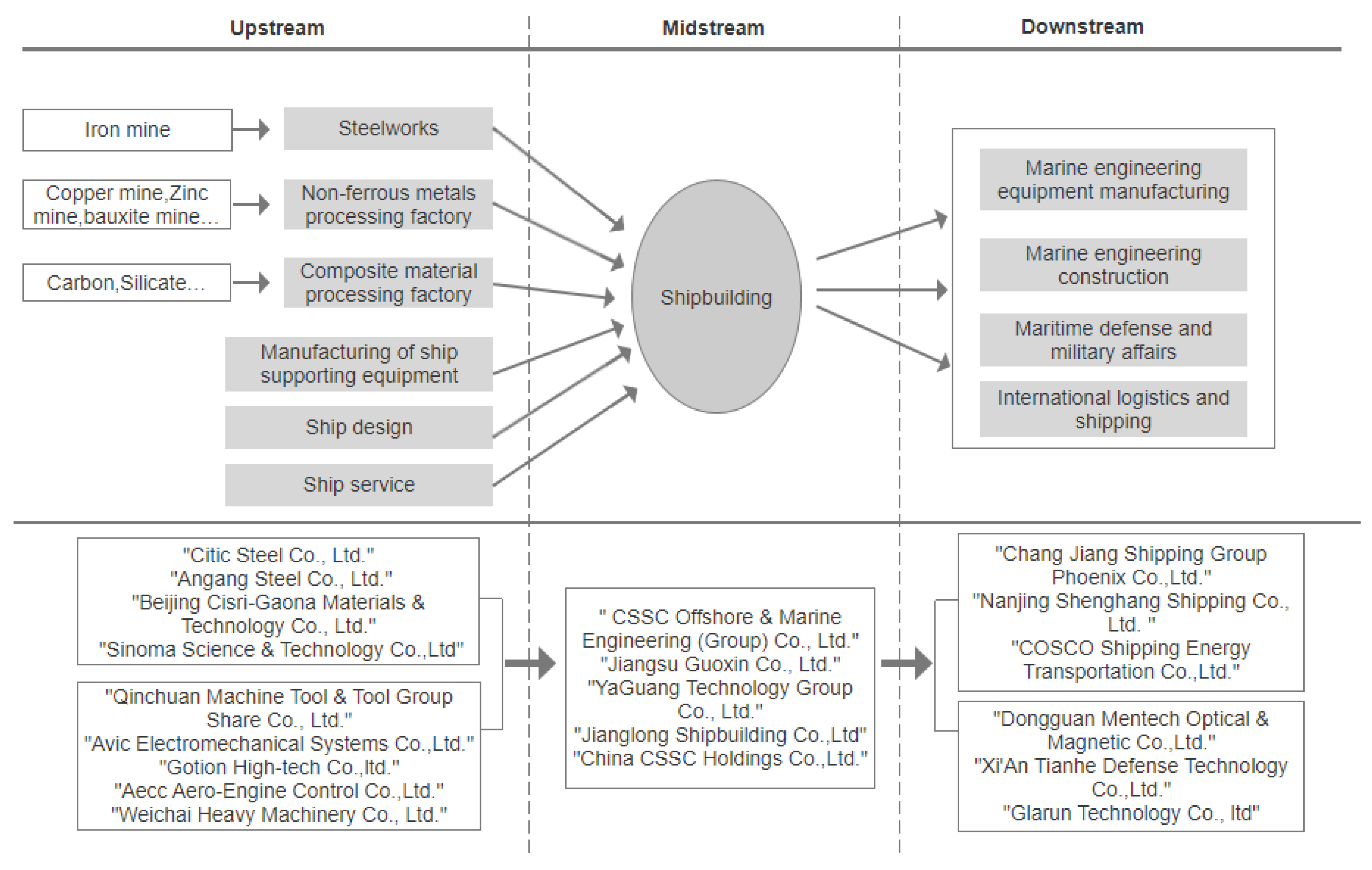
2.1. The Marine Ship Industry Chain

Scholars have unified the division of the upstream, midstream, and downstream of the marine ship industry chain. The upstream includes the supply of raw materials and marine supporting equipment, the midstream is shipbuilding, and the downstream is the application of ships [9,13,14]. Specifically, the upstream of the marine ship industry chain includes the supply of raw materials, such as steel, non-ferrous metals, and composite materials required for shipbuilding, as well as the manufacture of marine supporting equipment, such as marine engines, lighting equipment, navigation and communication equipment, ship paint, coatings, and ship design. The midstream of the industry chain covers the manufacture of various types of ships, such as large oil tankers, container ships, liquefied petroleum gas ships, liquefied natural gas ships, special chemical tankers, and luxury cruise ships, as well as the repair and maintenance of ships. The downstream of the industrial chain includes international logistics and shipping services, maritime defense and military affairs, marine engineering equipment manufacturing, and marine engineering construction. A schematic diagram of the marine ship industry chain is shown in Figure 1, which includes some representative enterprises corresponding to each link of the industry chain.

The existing literature on the marine ship industry chain is relatively scarce, but the research on the shipbuilding industry is abundant. The research on the shipbuilding industry in literature in recent years can be generally divided into four types.

One type of research studies the supply chain of the shipbuilding industry. For example, Caniëls, Cleophas, and Semeijn (2016) took environmental protection into account in the supply chain of the shipbuilding industry, and then analyzed the influencing factors of suppliers’ participation in green supply chain management [15]. Ferreira et al. (2018) made an empirical analysis of supply chain risk management in the Brazilian shipbuilding industry [16]. Ramirez-Peña et al. (2019) optimized the evaluation of the supply chain index to make the supply chain of the shipbuilding industry more suitable for Industry 4.0 [17]. Praharsi et al. (2021) took Indonesia’s traditional ship supply chain as the research object and used the supply chain operation reference index to measure its supply chain performance [18].

A second type of research is about the efficiency of the shipbuilding industry. There are several ways to study the efficiency of the shipbuilding industry. Qu (2014) [19] and Zhou and Guan (2019) [10] used the DEA-Malmquist model to calculate the total factor productivity of China’s shipbuilding industry based on regional data, and concluded that technical efficiency is the main driving force promoting the total factor productivity of China’s shipbuilding industry. Li, Zhang, and Liu (2017) [6] used stochastic frontier analysis to calculate the technical efficiency of the shipbuilding industry, and then further analyzed the regional development differences as well as the influencing factors of technical efficiency. Xue et al. (2020) [20] constructed a two-stage internal production efficiency structure analysis model (ESAM) to analyze the efficiency of the internal operation, process, and management of Chinese shipyards.

Thirdly, some scholars have studied the spatial layout of the shipbuilding industry. Liu, Shi, and Zeng (2017) [9] used GIS technology and spatial statistical methods; they found that China’s shipbuilding industry is concentrated in the Yangtze River economic belt and the eastern coastal cities. Shen, Li, and Shi (2018) [7] measured the total factor productivity of enterprises in China’s shipbuilding industry and then used a spatial econometric model to explore the differences in the spatial distribution of total factor productivity.

A fourth type of research studies the innovation ability of enterprises in the shipbuilding industry. Huang (2016) [21] studied the mode of independent innovation and collaborative innovation in China’s shipbuilding industry. Guo et al. (2021) [8] used entropy weight TOPSIS to evaluate the innovation ability of enterprises in China’s shipbuilding industry. In addition to the above, Barwick, Kalouptsidi, and Zahur (2021) [22] also used a dynamic model to evaluate the impact of different industrial policy tools on the development of China’s shipbuilding industry.

2.2. Calculation Methods of Industrial Chain Efficiency

A multi-stage data envelopment analysis (DEA) model is widely used in the research of industrial chain efficiency, including the one-stage DEA model, two-stage DEA model, three-stage DEA model, and so on. Firstly, the one-stage DEA model uses the DEA model to calculate the efficiency of the whole industrial chain and each of its links, or, combined with the Malmquist index model, to calculate and decompose the total factor productivity. Yan and Hou (2018) [23] sorted out the mining industry chain according to the different minerals and provincial mineral resources, and then used the traditional DEA model and super-efficiency DEA model to calculate the efficiency of the total mineral industry chain and different mineral industry chains. Tu, Xie, and Wang (2020) [24] used the network DEA model and Malmquist index model to measure the transformation efficiency and total factor productivity of China’s non-ferrous metal industry chain as a whole and at all stages. However, using the one-stage DEA model to study industrial chain efficiency has limitations. It cannot deeply analyze the factors affecting industrial chain efficiency, and the calculated industrial chain efficiency does not exclude the influence of environmental variables and statistical noise, which can lead to an overestimation or underestimation of efficiency values.

Compared with the one-stage DEA model, the two-stage DEA model can further explore how the objective environment and internal factors affect the efficiency of the industrial chain. The model uses the DEA model to measure the efficiency of the industrial chain in the first stage, and then uses the regression analysis method to analyze the factors affecting the efficiency in the second stage. For example, Liu et al. (2019) [25] used the two-stage DEA, which was composed of the chain relational network DEA model and the Tobit model, to measure the efficiency of the consulting and construction stage in the construction industry chain, as well as explore the influencing factors of the efficiency. Jiang and Liu (2021) [26] constructed a two-stage DEA model using DEA and the fixed-effect regression model, measured the production efficiency of China’s wind power industry chain and its links, and analyzed the impact of different policies on the efficiency of the industry chain. Chu et al. (2021) [27] also used the two-stage DEA model to measure the innovation efficiency of technology development and economic transformation in the innovation value chain of the Jiangsu National High-tech Zone, after which they explored the factors affecting innovation efficiency.

The three-stage DEA model goes further than the two-stage DEA model. After using the DEA model to measure the efficiency of the industrial chain in the first stage, the SFA method is used to adjust the slack variables of the input and output indicators in the second stage. In the third stage, the DEA model is used to calculate the industrial chain efficiency by using the adjusted input and output indicators. Compared with the efficiency value of the first stage, the efficiency value of the third stage excludes the influence of environmental factors and random error terms and can more accurately reflect the actual situation of the industrial chain efficiency. For instance, Li et al. (2020) [28] used the generalized three-stage DEA model to measure the technological innovation efficiency of each link of China’s integrated circuit industry chain based on provincial data. Luo and Lai (2021) [29] used the three-stage DEA model composed of the BCC model and the SFA model to measure the efficiency of China’s rare earth industry chain and each of its links. Zhao et al. (2022) [30] measured the input–output efficiency of China’s power generation enterprises using the three-stage DEA model. In addition, the three-stage DEA model combined with other methods can more accurately evaluate the efficiency and its influencing factors. Huang et al. (2022) [31] used the three-stage DEA model and AHP method to evaluate the performance of China’s energy supply chain under the “double-carbon” goal. Li et al. (2022) [32] analyzed the impact of transportation infrastructure on green buildings using the three-stage super-efficiency SBM model and Tobit model. Yan et al. (2022) [33] combined the three-stage super-efficiency SBM model with machine learning to study the main influencing factors of grain production efficiency in the Hexi Corridor of China.

With the research and innovation of non-parametric estimation methods, scholars have found that the multi-stage DEA model also has some inevitable defects. (1) It is deterministic. Since the DEA model is a deterministic frontier model, its effective boundary is determined by the sample observation results. Therefore, when calculating efficiency, if the input and output data of a decision-making unit have extreme values or outliers, it will affect the production frontier of the model construction, thereby affecting the DEA analysis results [34]. (2) It cannot deal with the statistical noise. The DEA model considers all inefficient decision-making units to be technical inefficiencies after determining the production frontier and, thus, does not divide inefficiencies into technical inefficiencies and random errors [35,36]. (3) DEA model has non-statistical properties. Since there are few premise assumptions for non-parametric estimation, it is difficult to make statistical inferences [34,37]. (4) The economic explanation parameters are insufficient. Due to the lack of parameter settings, it is difficult to explain the production process in terms of elasticity of substitution, marginal product, and partial elasticity [35].

Nonetheless, the advantages of the multi-stage DEA model and its derivatives are also more obvious. For example, to use the multi-stage SBM model is to propose the improvement direction for inefficient DMU. The analysis of the slack variables of input and output by the SBM method can further elucidate the resource usage of inefficient DMUs and propose the direction and size of improvement for inefficient resources, thus, providing decision makers with ways to improve efficiency [38,39]. Using the three-stage DEA model, we can use SFA to clarify the effect of environmental factors on efficiency in the second stage. Environmental influence factors and random error terms are then separated from the management inefficiency terms, and their influences are filtered out from the input and output data. In the end, we can obtain pure efficiency [40].

Our research aims to discover the problems existing in the development of industrial chain efficiency, as well as to clarify the direction of industrial chain efficiency improvement by analyzing the effect of environmental factors on industrial chain efficiency. Therefore, we selected the three-stage super-efficiency SBM model composed of the super-efficiency SBM model and the SFA method to deeply explore the mechanism of external factors affecting the overall efficiency of the industrial chain.

3. Empirical Methods

3.1. Three-Stage Super-Efficiency SBM Model

The maximum efficiency value of the decision-making units (DMUs) measured by the traditional DEA model (such as the CCR and the BCC model) is 1, so it is impossible to distinguish the DMUs whose efficiency value is greater than 1. Therefore, Andersen and Petersen (1993) proposed a super-efficiency DEA model to distinguish DMUs with efficiency values greater than 1 [41]. After that, Tone (2002) constructed the super-efficiency SBM model on the basis of the super-efficiency DEA model, which incorporated the relaxation variable into an objective function [42]. Fried et al. (2002) further proposed a three-stage DEA model combining the DEA and SFA [40]. The three-stage DEA model eliminates the impact of external environmental factors and statistical noise on the efficiency calculation of DMUs and improves the accuracy of the efficiency calculation of decision-making units.

On this basis, this paper combines the three-stage DEA model with the super-efficiency SBM model and draws on the relevant research of Wang, Dong, and Dong (2020) [43] to construct a three-stage super-efficiency SBM model. The model design is as follows.

In the first stage, we study the minimization of the input at a certain output level. Therefore, we first use the input-oriented super-efficiency SBM model [42] under the condition of constant returns to scale (CRS) to calculate the comprehensive technical efficiency value and input slack variables of each decision-making unit (DMU).

$$\begin{array}{l}min{\rho }_{TE}=1+\frac{1}{m}{\displaystyle \sum _{i=1}^m}\frac{S_i^{-}}{x_{i\mathrm{k}}}\\ \text{∣s.t.}\{\begin{array}{c}{x}_{ik}\ge {\displaystyle \sum _{j=1,\ne k}^n}{x}_{ij}{\lambda }_j\ge s_i^{-}(i=1,2,\dots ,m)\\ y_{rk}\le {\displaystyle \sum _{j=1,\ne k}^n}{y}_{rj}{\lambda }_j(r=1,2,\dots ,q)\\ {\lambda }_j\ge 0,s_i^{-}\ge 0\end{array}\end{array}$$

(1)

In Formula (1), ${\rho }_{TE}$ is the comprehensive technical efficiency value, $m$ is the number of input indicators, $q$ is the number of output indicators, and $n$ is the number of DMUs. Furthermore, $x_{ik}$ represents the value of the $i$th input indicator of the $k$th DMU, and $y_{rk}$ represents the value of the $r$th output indicator of the $k$th DMU. Additionally, $s_i^{-}$ is the slack variable of the $i$th input indicator, and ${\lambda }_j$ is the weight vector. If ${\rho }_{TE}$ ≥ 1, the DMU is relatively effective; if ${\rho }_{TE}$ < 1, the DMU is relatively ineffective.

The value of ${\rho }_{TE}$ calculated under the CRS is not pure technical efficiency value, and it includes a scale efficiency component. Therefore, by adding $\sum _{j=1,\ne k}^n{\lambda }_j=1$ to Formula (1), we can calculate the efficiency value in the case of variable returns to scale (VRS), as shown in Formula (2). The value of ${\rho }_{PTE}$ calculated in Formula (2) is the value of pure technical efficiency. Therefore, the scale efficiency can be obtained by calculating the ratio of ${\rho }_{TE}$ to ${\rho }_{PTE}$, that is, ${\rho }_{SE}$=${\rho }_{TE}$/${\rho }_{PTE}$.

$$\begin{array}{l}min{\rho }_{PTE}=1+\frac{1}{m}{\displaystyle \sum _{i=1}^m}\frac{S_i^{-}}{x_{ik}}\\ \text{∣s.t.}\{\begin{array}{c}{x}_{ik}\ge {\displaystyle \sum _{j=1,\ne k}^n}{x}_{ij}{\lambda }_j\ge s_i^{-}(i=1,2,\dots ,m)\\ y_{rk}\le {\displaystyle \sum _{j=1,\ne k}^n}{y}_{rj}{\lambda }_j(r=1,2,\dots ,q)\\ {\displaystyle \sum _{j=1,\ne k}^n}{\lambda }_j=1\\ {\lambda }_j\ge 0,s_i^{-}\ge 0\end{array}\end{array}$$

(2)

In the second stage, the SFA is adopted to eliminate the influence of environmental factors and random errors on the efficiency value of the DMUs. According to the method of Fried et al. (2002) [40], the slack variables of input indicators are respectively regressed with environmental variables. The regression models of slack variables and environmental variables are set as follows:

$$s_{ij}^{-}=f\left(Z_j,{\beta }_i\right)+v_{ij}+u_{ij},j=1,2,\cdots n,i=1,2\cdots m$$

(3)

$${\gamma }_{ }=\frac{{\sigma }_{u_{ }}^2}{{\sigma }_{v_{ }}^2+{\sigma }_{u_{ }}^2}$$

(4)

In Formula (3), $m$ is the number of input indicators, $n$ is the number of decision-making units, and $s_{ij}^{-}$ represents the slack value of the $i$th input of the $j$th DMU;$Z_j=\left[Z_{1j},\dots ,Z_{pj}\right]$ represents $p$ environmental variables of the $j$th DMU; ${\beta }_i=\left[{\beta }_{1i},\dots ,{\beta }_{pi}\right]$ is the regression coefficient to be estimated of $p$ environmental variables; $v_{ij}$ represents the random error term, and $v_{ij}\sim \left(0,{\sigma }_{v_{ }}^2\right)$; $u_{ij}$ represents the management inefficiency term, and $u_{ij}\sim \left(0,{\sigma }_{u_{ }}^2\right)$; $v_{ij}$ and $u_{ij}$ are independent of each other. In Formula (4), ${\gamma }_{ }$ is close to 1, which means that the main reason for the low efficiency of the DMU is management inefficiency, and ${\gamma }_{ }$ is close to 0, which means that the low efficiency of the DMU is caused by the random error terms.

Based on the research of Luo (2012) [44] and Chen et al. (2014) [45], this paper sets the formula for calculating the management inefficiency term $u_{ij}$ as follows:

$$E\left[u_{ij}\mid \left({\mathrm{v}}_{ij}+u_{ij}\right)\right]=\sigma \left[\frac{\mathsf{\Phi }\left(\frac{{\epsilon }_i\lambda }{\sigma }\right)}{\phi \left(\frac{{\epsilon }_i\lambda }{\sigma }\right)}+\frac{{\epsilon }_i\lambda }{\sigma }\right]$$

(5)

where $\lambda =\frac{{\sigma }_u}{{\sigma }_v}$, ${\epsilon }_i=v_{ij}+u_{ij}$, $\sigma =\sqrt{{\sigma }_u^2+{\sigma }_{\nu }^2}$, $\sigma$ represents the mixing error term, and $\mathsf{\Phi }$ and $\phi$ represent the probability density function and distribution function of standard normal distribution, respectively. To further separate the random error term from the mixed error term, we set it as Formula (6).

$$E\left[v_{ij}\mid \left(v_{ij}+u_{ij}\right)\right]=S_{ij}-f\left(Z_j,{\beta }_i\right)-E\left[u_{ij}\mid \left(v_{ij}+u_{ij}\right)\right]$$

(6)

After completing the separation of the random error term and the management inefficiency term, we can obtain the adjusted input value by bringing the random error term, the management inefficiency term, and the original input value into the following formula [45]. The adjustment formula is as follows:

$$\begin{gathered} X_{ij}^A=X_{ij}+\left[max\left(f\left(Z_j,{\widehat{\beta }}_i\right)\right)-f\left(Z_j,{\widehat{\beta }}_i\right)\right]+\left[max\left(v_{ij}\right)-v_{ij}\right] \\ j=1,2,\cdots n,i=1,2\cdots m \end{gathered}$$

(7)

where $X_{ij}^A$ is the adjusted input value, $X_{ij}$ is the initial input value, $max\left(f\left(Z_j,{\widehat{\beta }}_i\right)\right)-f\left(Z_j,{\widehat{\beta }}_i\right)$ means that all DMUs are in the same external environment, and $max\left(v_{ij}\right)-v_{ij}$ is used to adjust the random error items of all DMUs to the same state.

In the third stage, the super-efficiency SBM model [42] is applied to calculate the efficiency values of the DMUs by using the adjusted input values and initial output values. We can then obtain the efficiency excluding environmental factors and random error terms. The method steps are consistent with the first stage.

3.2. The Kernel Density Estimation Method

The kernel density estimation method can estimate the unknown probability distribution function and study the data distribution characteristics from the data itself [46,47]. Therefore, we use this method to analyze the distribution of efficiency of enterprises in the industrial chain. The model assumes that there are $n$ independent and identically distributed samples, $x_i$ is the observed value of the $i$th sample, $f\left(x\right)$ is the kernel density function of the random variable $x$, and the estimation formula of $f\left(x\right)$ is as follows:

$$f\left(x\right)=\frac{1}{nh}{{\displaystyle \sum }}_{i=1}^{n}K\left(\frac{x-x_i}{h}\right)$$

(8)

where $h$ is the bandwidth, and K(·) is a kernel density function that satisfies the conditions of non-negativity and the integral of 1. The commonly used kernel density functions include the triangular kernel function, gamma kernel function, and Gaussian kernel function. In this paper, the Gaussian kernel function is used for calculation.

4. Empirical Analysis

4.1. Variable Selection and Data Sources

Since we studied China’s marine ship industry chain from the micro level, we carried out the research based on enterprise data. In order to obtain open and complete annual report data of enterprises, we selected enterprises listed on A-Share in China’s securities market as the research objects, as these listed companies have to publish their annual reports every year to disclose their operating conditions to investors. Therefore, we could obtain complete business operation data, such as main business costs and management expenses, from the annual reports issued by listed enterprises. We could then use these data to calculate the efficiency of enterprises in each link of the marine ship industry chain.

Firstly, we obtained the name list of listed companies from the RESSET database (www.resset.com (accessed on 3 April 2022)). The data of listed companies in the RESSET database come from China’s Shanghai Stock Exchange and Shenzhen Stock Exchange. We selected representative companies in each link of the marine ship industry chain according to the following rules: (1) The stock code of the listed companies does not start with “PT” or “ST” and does not belong to the financial industry, since, according to the regulations of the China Securities Regulatory Commission, this means that the listed company has been operating poorly for more than two consecutive years, losing money continuously, and is at risk of being delisted. In addition, we chose listed companies that do not belong to the financial industry, in order to exclude the financial leasing companies related to ships. These companies do not have ships as fixed assets and are not included in the marine ship industry chain that we divided. (2) The company’s main business is highly related to the marine ship industry chain. By analyzing the main business content of the company, we excluded companies whose ship-related business is marginal. This ensures that the companies we choose are highly relevant to the marine ship industry chain. (3) The company’s financial statement data is continuous and complete.

After the above screening, a total of 79 representative listed companies in the upstream, midstream, and downstream of the industrial chain were selected. We then searched the CSMAR database for these companies’ financial statement data from 2015 to 2019. The data of the CSMAR database comes from authoritative statistical institutions, such as China’s Shenzhen Stock Exchange, the Shanghai Stock Exchange, the Shanghai Futures Exchange, and the National Bureau of Statistics. Moreover, we obtained the regional data required for environmental variables from the website of the National Bureau of Statistics (www.stats.gov.cn (accessed on 3 April 2022)).

We used MaxDEA software (Cheng, G. 2014. Data Envelopment Analysis: Methods and MaxDEA Software. Version 8.0. Intellectual Property Publishing House Co. Ltd., Beijing, China) to calculate the super-efficiency SBM model, and used Frontier software (Version 4.1. Coelli, T.J., Armidale, NSW, Australia) to calculate the SFA model. The selection of input and output indicators and environmental variables was performed as follows.

(1)

Input and Output Indicators

We selected the number of employees, main business costs, and management fees as input indicators and selected the main business income and total profits as output indicators. Among the input indicators, the number of employees represents the labor force invested by the enterprise in production and operation; the main business costs and enterprise management fees represent the capital investment of the enterprise. Among the output indicators, the main business income and total profits can show the production and operation capacity of the enterprise.

In order to ensure that the selected input indicators and output indicators conform to the isotropic principle, we used Stata software (Version 16.0. StataCorp LLC., College Station, TX, America) to conduct the Pearson correlation coefficient test for them. The test results (

Table 1. Pearson correlation coefficient test results.

	Main Business Income	Total Profits	Main Business Costs	Management Fees	The Number of Employees
Main business income	1.0000
Total profits	0.7211 ***	1.0000
Main business costs	0.9987 ***	0.6928 ***	1.0000
Management fees	0.8253 ***	0.5767 ***	0.8209 ***	1.0000
The number of employees	0.8267 ***	0.4577 ***	0.8290 ***	0.7985 ***	1.0000

Note: *** represents “significant” at significance levels of 1%.

) show that the input indicators have a significant positive impact on the output indicators and that they conform to the principle of contract orientation, indicating that the selection of input and output indicators is reasonable and effective.

(2)

Environmental Variables

We selected the level of economic development, the government support, the degree of regional openness, and the regional industrial structure as the environmental variables. These environmental variables have significant impacts on the survival environment of marine ship industry chain enterprises. (1) In regions with a high level of economic development, the market is vigorous. Product demand and market competition can promote industrial development. In addition, the economically developed regions can gather talents and technologies and have complete production factors. These factors can meet the development needs of enterprises. (2) Government support mainly refers to the government’s encouragement and support for local scientific and technological innovation. Strong government support is conducive to the formation of a good innovation atmosphere in the region. It can promote the technological innovation of industrial chain enterprises in high-tech manufacturing industries and further promote industrial technology upgrading. (3) A high degree of regional openness can promote the development of local import and export trade and is conducive to the marine ship industry chain to undertake orders for cargo transportation, equipment manufacturing, and shipbuilding at home and abroad. (4) Enterprises in each link of the marine ship industry chain are concentrated in the manufacturing field. The high proportion of the secondary industry in the regional industrial structure indicates that the regional manufacturing industry has a high degree of development and that the regional industrial system is relatively complete. This is conducive to the production and operation of enterprises in all links of the industry chain.

A description of each environmental variable is shown in

Table 2. Information on input indicators, output indicators, and environmental variables.

Variable Type	Variable Name	Specific Description of Variable	Unit	Data Sources
Input indicators	Labor input	Number of employees	People	CSMAR database
	Capital input	Main business costs	${10}^4$ Yuan	CSMAR database
		Management fees	${10}^4$ Yuan	CSMAR database
Output indicators	Enterprise income	Main business income	${10}^4$ Yuan	CSMAR database
		Total profits	${10}^4$ Yuan	CSMAR database
Environmental variables	The level of economic development	Provincial GDP	${10}^8$ Yuan	National Bureau of Statistics
	Government support	Provincial fiscal expenditure on science and technology	${10}^4$ Yuan	National Bureau of Statistics
	The degree of regional openness	Total provincial exports/provincial GDP × 100%	%	National Bureau of Statistics
	Regional industrial structure	Output value of provincial secondary industry / provincial GDP × 100%	%	National Bureau of Statistics

(the description of input and output indicators are also shown in Table 2).

4.2. Empirical Results

(1)

Stage 1: The Super-Efficiency SBM Model before Adjustment

Figure 2 shows the calculation results of TE, PTE, and SE of the upstream, midstream, and downstream of China’s marine ship industry chain from 2015 to 2019.

Figure 2 shows that, from 2015 to 2019, the TE, PTE, and SE of the upstream, midstream, and downstream of the marine ship industry chain have an upward trend in most years, except for a few years during which they have declined. Specifically, the three efficiency values’ improvement in 2018 increased significantly, but they fell in 2019. A detailed analysis of each picture, in Figure 2a,b, show that the TE value and PTE value of each link of the industrial chain are both low. The TE value is concentrated between 0.35 and 0.5, and the PTE value is generally between 0.5 and 0.65. None of them have reached the high-efficiency level and can still be improved. Moreover, by comparing the efficiency of each link, the TE and PTE of the upstream, midstream, and downstream of the industrial chain are distributed in a “V”-shape, high at both ends and low in the middle. The TE and PTE of the upstream and downstream are relatively high, but the midstream has become the trough of the industrial chain efficiency. Figure 2c shows that the SE value of the industrial chain is in the range of 0.65–0.85. After 2018, the scale efficiency value of each link of the industrial chain exceeded 0.7. This is a relatively high-efficiency level. Unlike the “V”-shaped distribution, the SE values of the upstream, midstream, and downstream of the industrial chain show a one-sided trend of upstream > midstream > downstream. The rising range of the midstream and downstream is greater than that of the upstream year by year, but the upstream always maintains a leading position due to its high starting point.

In general, the low TE of each link of the industrial chain is mainly restrained by PTE, while SE is the main driving force for the development of TE. By further calculating the average efficiency of the upstream, midstream, and downstream of the industrial chain from 2015 to 2019 (Figure 3), it was found that the upstream shows obvious efficiency advantages; especially in 2018, it is in an absolute leading position. Followed by the downstream, its average efficiency is greater than 0.5, making slow progress above the medium-efficiency level. The midstream has always been in a state of inefficiency; the efficiency value is far lower than the upstream and downstream. This proves that the midstream has become the short board of the overall efficiency of the industrial chain. The midstream is mainly shipbuilding and is the core of the industry chain. It has become the short board, which will seriously hinder the development of the industrial chain. To this end, it is necessary to accelerate the research and development of key shipbuilding technologies, deeply integrate shipbuilding with emerging information technologies, and break through the technical weakness, so that the midstream can truly become the core connecting what precedes and follows it and, thus, lead the overall transformation and upgrading of the industrial chain with intelligent manufacturing.

In order to further analyze the microstructure and time trend of the efficiency of each link, we estimated the kernel density distribution of the enterprise efficiency of each link in the industrial chain from 2015 to 2019 (Figure 4).

As Figure 4a shows, the kernel density distribution curve of the upstream enterprise efficiency moves to the right from 2015 to 2019 and gradually changes from a single peak to double peaks, indicating that the efficiency level of upstream enterprises is constantly improving, and the efficiency difference between enterprises is increasing. Low-efficiency and high-efficiency enterprises show a gradual polarization. The kernel density distribution curves of midstream and downstream enterprise efficiency (Figure 4b,c) show that they maintain a single peak state and gradually move to the right, which means that the efficiency level of most enterprises in the midstream and downstream have been improved, but the difference of most enterprises’ efficiency is not obvious. In addition, in 2015, the upstream and downstream kernel density curves trail longer on the right side, which is due to the fact that the AVIC Electromechanical Company (Tianjin, China) in the upstream and the China Merchants Shipping Company (Beijing, China) in the downstream are significantly more efficient than other companies.

(2)

Stage 2: SFA Model Analysis

We then took the three-input slack variables obtained in the first stage as dependent variables, and used them for SFA regression with the four following independent variables: the level of economic development, government support, the degree of regional openness, and the regional industrial structure. The results are shown in

Table 3. Results of SFA regression.

	Slack Variable of Main Business Costs	Slack Variable of Management Fees	Slack Variable of Number of Employees
Constant term	60,373.6830 ***	−20430.5440 ***	−3737.3830 ***
The level of economic development	6.9402 ***	0.8883 ***	0.0387
Government support	−0.0363	−0.0058 ***	−0.0008 *
The degree of regional openness	−6759.7631 ***	−103.9413 ***	58.6994
Regional industrial structure	559.2412 ***	184.5237	136.8167 ***
${\sigma }^2$	6.0803 × 1011 ***	7.8633 × 109 ***	2.0663 × 108 ***
${\gamma }^{ }$	0.3687 ***	0.6439 ***	0.7586 ***
LR	24.1032 ***	99.0837 ***	164.7311 ***
LR	24.1032 ***	99.0837 ***	164.7311 ***

Note: *** and * represent “significant” at significance levels of 1% and 10%, respectively.

.

The significance of the regression coefficients in Table 3 shows that most of the environmental variables have significant impacts on the input slack variables, indicating that the selected environmental variables are more appropriate. The ${\gamma }^{}$ value of the model is close to 1 and is significant at the 1% level, showing that the input slack variables are greatly affected by environmental variables, so it is necessary to eliminate the influence of the objective environment and random error terms on the efficiency. The likelihood ratio test value LR is significant at the 1% level, which proves that the model setting is effective.

Since the influence of environmental variables on input slack variables is opposite to that on efficiency, the effect of environmental variables on efficiency can be judged by the symbol of the regression coefficient. (1) The regression coefficients of the level of economic development in relation to the slack variables of main business costs and management fees are all positive; that is, the economic development level has a negative impact on the efficiency of the marine ship industry chain. This might be because the high price of raw materials and the salary level of employees in economically developed areas lead to the high cost of enterprises. When the output remains unchanged, the enterprise cost is relatively high, resulting in a decline in efficiency. (2) The regression coefficients of government support in relation to the three input slack variables are negative. This means that government support has a significant impact on the input slack variables of management fees and the number of employees, indicating that a good scientific and technological innovation environment and strong government support can help to reduce input redundancy and improve the production and operation efficiency of the marine ship industry chain. (3) The degree of regional openness has a significant negative impact on the slack variables of main business costs and management fees, indicating that improving the degree of regional openness can help reduce the redundancy of costs and expenses, and improve the efficiency of enterprises in the marine ship industry chain. (4) The regional industrial structure has a significant positive impact on the slack variables of the main business cost and the number of employees. That is, the higher the proportion of the secondary industry, the lower the efficiency of the enterprise. This result shows that accelerating the optimization and upgrading of the industrial structure is of great significance in improving the efficiency of enterprises.

(3)

Stage 3: The Super-Efficiency SBM Model after Adjustment

We then used the adjusted input indicators and initial output indicators to calculate the TE, PTE, and SE of the upstream, midstream, and downstream of the industrial chain after excluding environmental factors and random error terms. The results are shown in Figure 5.

As Figure 5 shows, the values and distribution characteristics of the three efficiencies obviously change after adjustment. From the perspective of the adjusted TE of the industrial chain, the TE value of each link has declined substantially, and it is concentrated in the range of 0.1–0.3. The TE value in the downstream shows the largest decline. The distribution trend of three links has changed from the “V”-shape before adjustment to the echelon decreasing distribution of upstream > midstream > downstream (except in 2015). However, the PTE values of the three links after adjustment have been significantly improved compared to before the adjustment. The PTE values of the upstream and downstream are concentrated between 0.75 and 0.85, and the PTE values of the midstream are concentrated around 0.6. Obviously, there is still in a “V”-shaped distribution after adjustment, and midstream is still the trough of PTE in the industry chain. The SE value of each link has dropped significantly, from about 0.8 before the adjustment to about 0.3 after the adjustment. Although the gap between upstream and midstream has narrowed significantly after the adjustment, it is still in the order of upstream > midstream > downstream (except in 2015). After further calculating the adjusted average efficiency of each link (see Figure 6), the upstream is still in the leading position. On the contrary, the downstream now appears to be the weak link in terms of industrial chain efficiency, because the midstream is slightly ahead of the downstream after adjustment.

The difference in the TE of the industrial chain before and after adjustment reflects serious problems in the industrial chain, such as redundant investment and unreasonable resource allocation. The PTE rises instead of falling after excluding environmental factors, which reflects the technological innovation advantages of China’s marine ship industrial chain. This mainly benefits from the high-tech manufacturing enterprises in the industrial chain. Most of these enterprises have a high level of science and technology, and they are concentrated in developed coastal areas (such as the Guorui Technology Company (Jiangsu, China) and the Baoding Technology Company (Zhejiang, China)). These enterprises are key in leading the overall transformation and upgrading of the industrial chain and enhancing the core competitiveness of the industrial chain. Moreover, the decline of SE after adjustment reflects the problems of “big but not strong” and “small but not refined”, as well as the insignificant agglomeration effect of industrial chain enterprises. It is urgent that the overall spatial layout of the industrial chain be optimized and that the scale benefits be improved.

Figure 7 shows the kernel density distribution of enterprise efficiency in each link of the industrial chain after adjustment. Compared with the “thin and tall” shape of the density curve before the adjustment, the main peak of the enterprise efficiency density curve in each link after the adjustment is shorter and wider, indicating that the difference in efficiency between enterprises becomes larger. At the same time, the position of the main peak after the adjustment is more to the left than before the adjustment, which shows that, after the second stage of adjustment, the efficiency of most enterprises in all links has been reduced.

4.3. Coupling Coordination Analysis

In order to analyze the coordinated development between each link of the industrial chain, we further calculated the coupling degree and coupling coordination degree of the upstream–midstream and midstream–downstream in China’s marine ship industry chain. The coupling degree refers to the strength of mutual restriction or interdependence between the upstream and midstream, as well as the midstream and downstream. The calculation formula is as follows:

$$\{\begin{array}{c}{C}_1=2\times {\left[\frac{U_1\times U_2}{{\left(U_1+U_2\right)}^2}\right]}^{1/2}\\ C_2=2\times {\left[\frac{U_2\times U_3}{{\left(U_2+U_3\right)}^2}\right]}^{1/2}\end{array},\{\begin{array}{c}{U}_1=\left(T{E}_1+PT{E}_1+S{E}_1\right)/3\\ U_2=\left(T{E}_2+PT{E}_2+S{E}_2\right)/3\\ U_3=\left(T{E}_3+PT{E}_3+S{E}_3\right)/3\end{array}$$

(9)

where $C_1$ and $C_2$ represent the coupling degree of the upstream–midstream and midstream–downstream, respectively; $U_1$, $U_2$, and $U_3$ represent the evaluation values of the upstream, midstream, and downstream of the industrial chain, respectively. This paper uses the mean value of the efficiency measured in the third stage. On the basis of the coupling degree, the coupling coordination degree further reflects the degree of benign coupling in the interaction relationship between the two links, and reflects the level of coordinated development. The calculation formula is as follows:

$$\{\begin{array}{c}{D}_1=\sqrt{C_1\times T_1},T_1=\left(U_1+U_2\right)/2\\ D_2=\sqrt{C_2\times T_2},T_2=\left(U_2+U_3\right)/2\end{array}$$

(10)

In Formula (10), $D_1$ and $D_2$ represent the coupling coordination degree of upstream–midstream and midstream–downstream, respectively. Furthermore, $T_1$ and $T_2$ represent the coordination value of upstream–midstream and midstream–downstream, respectively. In this paper, the coupling degree value and coupling coordination degree value are divided into grades based on relevant research [48]. The value range and corresponding grades are shown in

Table 4. Classification of the coupling degree and the coupling coordination degree.

Value of C	Grade of C	Value of D	Grade of D
(0.0–0.3)	Separation stage	(0.0–0.2)	Extreme incoordination
[0.3–0.5)	Antagonistic stage	[0.2–0.4)	Moderate incoordination
[0.5–0.8)	Grinding-in stage	[0.4–0.6)	Basic coordination
[0.8–1.0)	Highly coupled stage	[0.6–0.8)	Moderate coordination
——	——	[0.8–1.0)	Superior coordination

Note: “C” represents the coupling degree; “D” represents the coupling coordination degree.

.

The calculation results are shown in

Table 5. Results of the coupling degree and the coupling coordination degree.

Year	Upstream—Midstream			Midstream—Downstream
	Value of C	Value of D	Grade	Value of C	Value of D	Grade
2015	1	0.651	Highly coupled and moderately coordinated	1	0.648	Highly coupled and moderately coordinated
2016	0.994	0.631	Highly coupled and moderately coordinated	0.999	0.61	Highly coupled and moderately coordinated
2017	0.991	0.654	Highly coupled and moderately coordinated	0.998	0.628	Highly coupled and moderately coordinated
2018	0.993	0.634	Highly coupled and moderately coordinated	1	0.603	Highly coupled and moderately coordinated
2019	0.995	0.666	Highly coupled and moderately coordinated	0.999	0.646	Highly coupled and moderately coordinated

Note: “C” represents the coupling degree; “D” represents the coupling coordination degree.

. The coupling degree of upstream–midstream and midstream–downstream of China’s marine ship industry chain are greater than 0.9, which is in a highly coupled stage. However, the coupling coordination degree is relatively low, as it is about 0.6 as a whole. There is no obvious improvement trend from 2015 to 2019. It can be said that the improvement of the coordination level is stagnant. The upstream and the midstream, as well as the midstream and the downstream, are all in a moderate coordination stage. The coordination between each link can still be improved. Generally speaking, after years of development, the links in China’s marine ship industry chain have completed a grinding-in. They are closely connected with each other and have entered a stage of high coupling. However, the degree of coordination of the upstream–midstream and midstream–downstream still needs to be improved, and the links have not achieved a highly synchronized development. In addition, the improved speed of the coordination degree is still very slow, indicating that the adjustment pace of each link in the industrial chain is inconsistent, and the self-coordination ability within the industrial chain is not strong. This means that, in the face of the impact of external environmental changes, all links of the industrial chain may lose synchronization, resulting in the poor anti-risk ability of the industrial chain.

5. Conclusions and Policy Implications

5.1. Conclusions

Based on the data of 79 listed companies in the marine ship industry from 2015 to 2019, we used the three-stage super-efficiency SBM model to calculate the TE, PTE, and SE of each link in China’s marine ship industry chain. We compared and analyzed the changes in the efficiency of the industry chain before and after excluding environmental variables and random error terms, and deeply explored the efficiency weaknesses of the industry chain as well as the coordinated development level of all links. The research found the following:

(1)

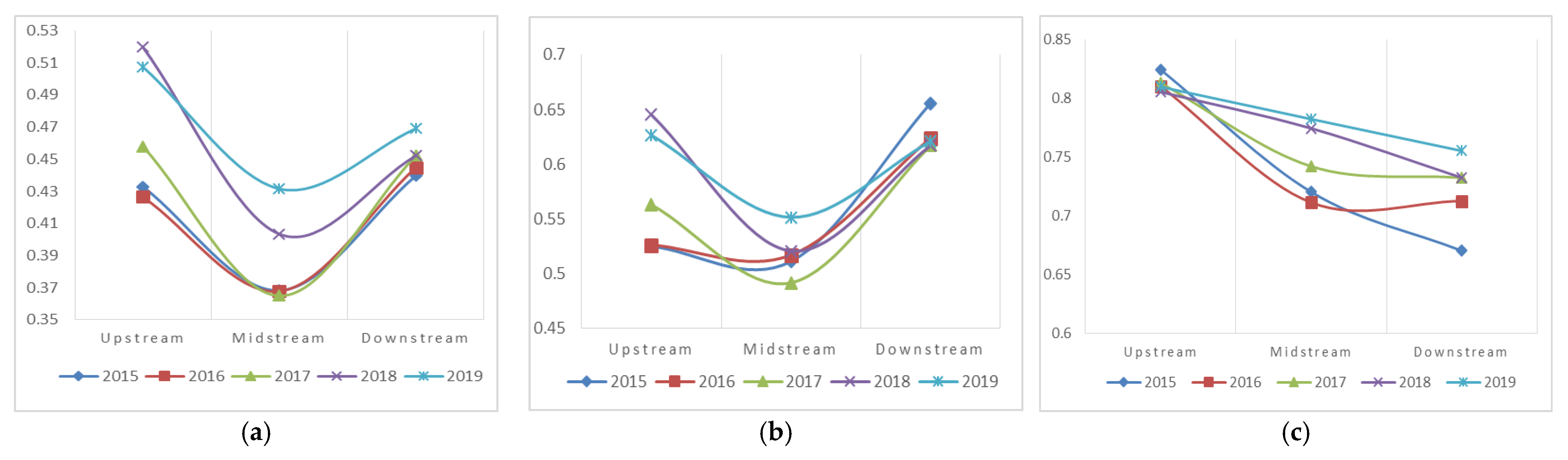
Before excluding the influence of environmental factors, the efficiencies of the upstream, midstream, and downstream of China’s marine ship industry chain have a “V”-shaped distribution in terms of comprehensive technical efficiency and pure technical efficiency, high at both ends and low in the middle. The efficiency of the midstream is significantly lower than that of the upstream and downstream, appearing as a weak link in terms of the efficiency of the industrial chain. The “V”-shaped distribution of the industrial chain efficiency is not conducive to the development of the industrial chain, since the shipbuilding industry in the midstream is the core link of the industrial chain. If the efficiency of the midstream continues to remain lower than that of the upstream and downstream, it will be difficult to drive the overall efficient operation of the industrial chain and this will limit the development of the industrial chain;

(2)

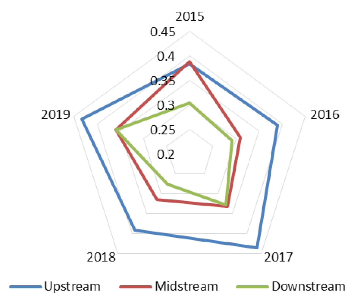
The scale efficiency value of each link of the industrial chain is at a medium–high level, and this is the main driving force promoting the comprehensive technical efficiency of the industrial chain. Specifically, the scale efficiency of each link of the industrial chain is distributed in the order of upstream > midstream > downstream; the scale efficiency is lowest in the downstream of the industrial chain. The existing industrial scale of downstream industries is not economical, which hinders downstream industries from achieving economies of scale;

(3)

The results of SFA regression show that environmental variables have significant impacts on the efficiency of the marine ship industry chain. Among them, the existing government support and the degree of regional openness have positive impacts on the efficiency of the industrial chain, so continuing to implement the current policy can effectively promote improvement in industrial efficiency. However, the impacts of the level of economic development and the regional industrial structure on industrial chain efficiency are negative. Therefore, it is necessary to focus on solving the problems related to these two aspects. Optimizing the industrial structure and accelerating industrial transformation and upgrading are important ways to improve the efficiency of the industrial chain;

(4)

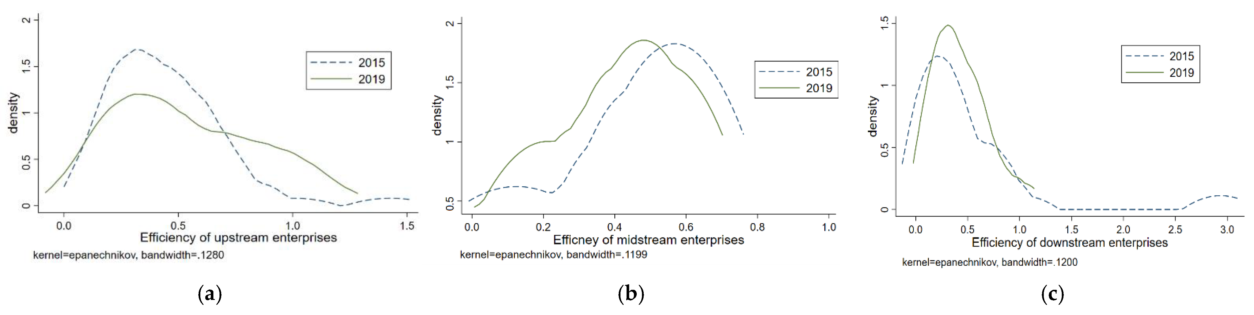
After eliminating the environmental impact factors and random interference items, the efficiency of each link in the industrial chain significantly changes. The level of pure technical efficiency increases significantly, and the scale efficiency clearly drops. This shows that the pure technical efficiency of each link of the industrial chain is substantially underestimated before environmental factors are excluded. Technological innovation and management system reform are also needed to improve the efficiency of the industrial chain;

(5)

In addition, the poor coordination among links in the industrial chain also limits the development of its efficiency. The coupling degree of upstream–midstream and midstream–downstream is high, but their coordination degree is low, and efficient synergy has not yet been achieved among all links in the industrial chain. Moreover, the improvement of the coordination degree of the industrial chain is very slow, and there is no clear trend of improvement. Therefore, strengthening the coordination and cooperation of all links in the industrial chain is also key in improving the efficiency of the industrial chain.

5.2. Policy Implications

In view of the reasons for restricting the development of industrial chain efficiency, we believe that the improvement of industrial chain efficiency can be carried out as follows:

(1)

We need to strengthen the technological collaborative innovation among the upstream, midstream, and downstream of the industrial chain, extend the technological advantages of the upstream to the midstream and downstream, and promote the technological progress of all links of the industrial chain with the help of a technology spillover effect. As weak links in terms of industrial chain efficiency, the midstream and downstream of the industrial chain should increase the learning and transformation of advanced management experience and technical knowledge, optimize the weakness in their production and operation processes, improve the level of efficiency, and supplement the weaknesses in industrial chain development. In addition, the cooperation between enterprises among all links of the industrial chain and regional research institutions and universities need to be strengthened, breakthroughs in key and difficult technologies and the transformation of technological innovation achievements need to be promoted, and the technical strength of the industrial chain, with the help of the strengths of all parties, must be enhanced;

(2)

It is important to improve the spatial planning and optimize the layout of the marine ship industry chain. In order to achieve economies of scale, we should improve the supporting facilities, concentrate on the production factors required for industrial development, and promote the agglomeration and development of the marine ship industry in the region. Moreover, the cooperation and exchanges among all links of the industrial chain in the region need to be strengthened, and the formation of alliances between enterprises must be promoted. It is important to accelerate the flow of products and information between links and to improve the coordination and cooperation of production and operation in each link of the industrial chain;

(3)

The government should strengthen policy encouragement and support for technological innovation of enterprises in all links of China’s marine ship industry chain, break foreign technical barriers, promote the introduction of advanced technology, and help the industry achieve transformation and upgrading. At the same time, it should accelerate the conversion of the manufacturing industry in the region from old to new kinetic energy, optimize links with high amounts of consumption and pollution in the traditional industrial structure, and improve industrial efficiency. The government should promote the integration of emerging technologies, such as big data, the Internet of things, and artificial intelligence, with the marine ship industry chain and build a smart marine ship industry chain.

5.3. Research Deficiencies and Prospects

We identified the problems and constraints in the efficiency development of the links in China’s marine ship industry chain, but improvements in this research can be made. First, the sample data selected in this paper only include listed enterprises in the industrial chain, and the unlisted enterprises in the industrial chain were not observed. Moreover, the multi-stage DEA model has some defects, such as the fact that it is deterministic and doesn’t deal with the statistical noise. Therefore, in the next step of our research, we intend to use the advanced robust and nonparametric methods [35] to measure efficiency.

References

1. Gülmez, S.; Şakar, G.D.; Baştuğ, S. An overview of maritime logistics: Trends and research agenda. Marit. Policy Manag. 2021, 1–20. [Google Scholar] [CrossRef]
2. Shi, W.; Xiao, Y.; Chen, Z.; McLaughlin, H.; Li, K.X. Evolution of green shipping research: Themes and methods. Marit. Policy Manag. 2018, 45, 863–876. [Google Scholar] [CrossRef]
3. Zheng, D.; Zhang, Z.; Yu, J. Discussion on the Theory of Industrial Chain Integration. Sci. Technol. Prog. Policy 2011, 28, 64–68. [Google Scholar] [CrossRef]
4. Guo, X.; Li, L. Choice of Strategic Adjustment on China’s Shipbuilding Industry in Post-crisis Era. J. Jiangsu Univ. Sci. Technol. (Soc. Sci. Ed.) 2010, 10, 29–33. [Google Scholar] [CrossRef]
5. Xu, J. Strategic Thinking on Development of Chinese Shipbuilding Industry. China Ind. Econ. 2002, 12, 48–56. [Google Scholar] [CrossRef]
6. Li, G.; Zhang, G.; Liu, J. Regional Differences and Convergence Analysis of Technical Efficiency of Shipbuilding Industry in China. Shipbuild. China 2017, 58, 165–177. [Google Scholar]
7. Shen, T.; Li, S.; Shi, X. Research on the Spatial Pattern and Influence Factors of Total Factor Productivity of Shipbuilding Industry in China. Mar. Econ. 2018, 8, 45–55. [Google Scholar] [CrossRef]
8. Guo, T.; Wang, S.; Li, P. Evaluation of Innovation Ability of Chinese Shipbuilding Listed Companies from the Perspective of Civil-Military Integration. Oper. Res. Manag. Sci. 2021, 30, 114–120. [Google Scholar] [CrossRef]
9. Liu, H.; Shi, Y.; Zeng, C. Spatial Layout and Development Strategy of the Ship-Related Industry in China. Econ. Geogr. 2017, 37, 99–107. [Google Scholar] [CrossRef]
10. Zhou, Z.; Guan, H. Analysis of Total Factor Productivity and Influencing Factors in China’s Shipbuilding Industry: Based on Industrial Environment Perspective. Ocean Dev. Manag. 2019, 36, 114–120. [Google Scholar]
11. Fang, C.; Guan, X. Comprehensive Measurement and Spatial Distinction of Input-output Efficiency of Urban Aqqlomerations in China. Acta Geogr. Sin. 2011, 66, 1011–1022. [Google Scholar]
12. Yang, L.; Wang, X. The Efficiency of Non-ferrous Metals Industry Chain in China and Influencing Factors—Two-stage Analysis Based on Network DEA Model. Reform. Strategy 2018, 34, 102–109. [Google Scholar] [CrossRef]
13. Tan, S.; Yan, K. Evaluation Research of China Regional Shipbuilding Competitiveness in Global Value Chain. J. Ind. Technol. Econ. 2011, 30, 24–30. [Google Scholar] [CrossRef]
14. Su, Y.; Wang, F.-Y.; An, X.-L. Coupling Mechanism and Coupling Degree Measurement Model of Shipbuilding Industry Cluster. Pol. Marit. Res. 2016, 23, 78–85. [Google Scholar] [CrossRef]
15. Caniëls, M.C.J.; Cleophas, E.; Semeijn, J. Implementing green supply chain practices: An empirical investigation in the shipbuilding industry. Marit. Policy Manag. 2016, 43, 1005–1020. [Google Scholar] [CrossRef]
16. Ferreira, F.D.A.L.; Scavarda, L.F.; Ceryno, P.S.; Leiras, A. Supply chain risk analysis: A shipbuilding industry case. Int. J. Logist. Res. Appl. 2018, 21, 542–556. [Google Scholar] [CrossRef]
17. Ramirez-Peña, M.; Fraga, F.J.A.; Sotano, A.J.S.; Batista, M. Shipbuilding 4.0 Index Approaching Supply Chain. Materials 2019, 12, 4129. [Google Scholar] [CrossRef]
18. Praharsi, Y.; Abu Jami’In, M.; Suhardjito, G.; Reong, S.; Wee, H.M. Supply chain performance for a traditional shipbuilding industry in Indonesia. Benchmarking Int. J. 2021, 29, 622–663. [Google Scholar] [CrossRef]
19. Qu, Y. The Productivity Growth and Convergence Analysis on Shipbuilding Industry in China. J. Hebei Univ. Econ. Bus. 2014, 35, 116–120. [Google Scholar] [CrossRef]
20. Xue, L.; Shi, G.; Dai, D.; Xu, Y. Two-Stage Efficiency Structure Analysis Model of Shipbuilding Based on Driving Factors: The Case of Chinese Shipyard. Open J. Soc. Sci. 2020, 08, 182–200. [Google Scholar] [CrossRef]
21. Huang, H. Research on the new mode of independent innovation and collaborative innovation based on industry convergence. Sci. Manag. Res. 2016, 34, 42–45. [Google Scholar] [CrossRef]
22. Barwick, P.J.; Kalouptsidi, M.; Zahur, N.B. Industrial Policy Implementation: Empirical Evidence from China’s Shipbuilding Industry; Cato Institute: Washington, DC, USA, 2021. [Google Scholar]
23. Yan, J.; Hou, M. Study on technology efficiency and spatial-temporal characteristics of mineral resources industry chains in China. China Min. Mag. 2018, 27, 65–69. [Google Scholar]
24. Tu, N.; Xie, R.; Wang, X. Study on the transformation efficiency of China’s non-ferrous metal industrial chain. China Min. Mag. 2020, 29, 32–39. [Google Scholar] [CrossRef]
25. Liu, B.; Wang, M.; Li, L.; Wang, R.; Meng, J. Research on Comprehensive Efficiency, Pure Technical Efficiency and Scale Efficiency of Two Stages of Chinese Construction Industry Chain and Their Influencing Factors. Oper. Res. Manag. Sci. 2019, 28, 174–183. [Google Scholar] [CrossRef]
26. Jiang, Z.; Liu, Z. Can wind power policies effectively improve the productive efficiency of Chinese wind power industry? Int. J. Green Energy 2021, 18, 1339–1351. [Google Scholar] [CrossRef]
27. Chu, S.; Wang, T.; Xia, S.; Yang, X.; Chen, J. Differences and Influencing Factors of Enterprise Innovation Efficiency Based on Innovation Value Chain: A Case Study on Enterprises of National High-tech Zones in Jiangsu Province. Resour. Environ. Yangtze Basin 2021, 30, 269–279. [Google Scholar] [CrossRef]
28. Li, H.; He, H.; Shan, J.; Cai, J. Research on technology innovation efficiency of China’s IC industry eliminating the influence of non-operating factors: Analysis based on generalized GRA-DEA and Tobit. J. Ind. Eng. Eng. Manag. 2020, 34, 60–70. [Google Scholar] [CrossRef]
29. Luo, X.; Lai, D. Measuring and Comparing the Efficiency of the Whole Industry Chain of Rare Earths from the Perspective of Industry Chain Extension: Based on Three-Stage DEA Model. Sci. Decis. Mak. 2021, 06, 104–121. [Google Scholar] [CrossRef]
30. Zhao, W.; Qiu, Y.; Lu, W.; Yuan, P. Input–Output Efficiency of Chinese Power Generation Enterprises and Its Improvement Direction-Based on Three-Stage DEA Model. Sustainability 2022, 14, 7421. [Google Scholar] [CrossRef]
31. Huang, X.; Lu, X.; Sun, Y.; Yao, J.; Zhu, W. A Comprehensive Performance Evaluation of Chinese Energy Supply Chain under Double-Carbon Goals Based on AHP and Three-Stage DEA. Sustainability 2022, 14, 10149. [Google Scholar] [CrossRef]
32. Li, G.; Ma, X.; Song, Y. Green Building Efficiency and Influencing Factors of Transportation Infrastructure in China: Based on Three-Stage Super-Efficiency SBM–DEA and Tobit Models. Buildings 2022, 12, 623. [Google Scholar] [CrossRef]
33. Yan, Z.; Zhou, W.; Wang, Y.; Chen, X. Comprehensive Analysis of Grain Production Based on Three-Stage Super-SBM DEA and Machine Learning in Hexi Corridor, China. Sustainability 2022, 14, 8881. [Google Scholar] [CrossRef]
34. Simar, L.; Wilson, P.W. Sensitivity Analysis of Efficiency Scores: How to Bootstrap in Nonparametric Frontier Models. Manag. Sci. 1998, 44, 49–61. [Google Scholar] [CrossRef]
35. Daraio, C.; Simar, L. Advanced Robust and Nonparametric Methods in Efficiency Analysis: Methodology and Applications; Springer: Berlin/Heidelberg, Germany, 2007; pp. 3–7. [Google Scholar]
36. Nepomuceno, T.C.; Santiago, K.T.; Daraio, C.; Costa, A.P. Exogenous crimes and the assessment of public safety efficiency and effectiveness. Ann. Oper. Res. 2022, 316, 1349–1382. [Google Scholar] [CrossRef]
37. Bădin, L.; Daraio, C.; Simar, L. Explaining inefficiency in nonparametric production models: The state of the art. Ann. Oper. Res. 2014, 214, 5–30. [Google Scholar] [CrossRef]
38. Tone, K. A slacks-based measure of efficiency in data envelopment analysis. Eur. J. Oper. Res. 2001, 130, 498–509. [Google Scholar] [CrossRef]
39. Shen, C.; Zhang, D. Research on the Government’s Optimization of the Allocation of Scientific and Technological Resources; Peking University Press: Beijing, China, 2013; pp. 96–97. [Google Scholar]
40. Fried, H.O.; Lovell, C.K.; Schmidt, S.S.; Yaisawarng, S. Accounting for Environmental Effects and Statistical Noise in Data Envelopment Analysis. J. Product. Anal. 2002, 17, 157–174. [Google Scholar] [CrossRef]
41. Andersen, P.; Petersen, N.C. A procedure for ranking efficient units in data envelopment analysis. Manag. Sci. 1993, 39, 1261–1264. [Google Scholar] [CrossRef]
42. Tone, K. A slacks-based measure of super-efficiency in data envelopment analysis. Eur. J. Oper. Res. 2002, 143, 32–41. [Google Scholar] [CrossRef]
43. Wang, Q.; Dong, Y.; Dong, Y. Evaluation on Efficiency of Fiscal Expenditure for Science and Technology on the Background of the Strategy of Innovation-driven Development: Based on Three-stage Super-efficiency SBM-DEA Model. Sci. Technol. Manag. Res. 2020, 40, 23–33. [Google Scholar] [CrossRef]
44. Luo, D. A Note on Estimating Managerial Inefficiency of Three-Stage DEA Model. Stat. Res. 2012, 29, 104–107. [Google Scholar] [CrossRef]
45. Chen, W.; Zhang, L.; Ma, T. Research on Three-stage DEA Model. Syst. Eng. 2014, 32, 144–149. [Google Scholar]
46. Wang, X.; Chu, T. Non-Parametric Statistics, 2nd ed.; Tsinghua University Press: Beijing, China, 2014; pp. 213–218. [Google Scholar]
47. Wang, F.H. Quantitative Methods and Socio-Economic Applications in GIS; CRC Press: Boca Raton, FL, USA, 2015; pp. 176–180. [Google Scholar] [CrossRef]
48. Wang, C.; Tang, N. Spatio-temporal characteristics and evolution of rural production living-ecological space function coupling coordination in Chongqing Municipality. Geogr. Res. 2018, 37, 1100–1114. [Google Scholar] [CrossRef]
Figure 1. Schematic diagram of the marine ship industry chain.
Sustainability 14 12155 g001
Figure 2. Efficiency of each link in the marine ship industry chain over 2015–2019. (a) TE of each link; (b) PTE of each link; (c) SE of each link.
Sustainability 14 12155 g002
Figure 3. Short board analysis of the marine ship industry chain over 2015–2019.
Sustainability 14 12155 g003
Figure 4. Kernel density distribution of enterprise efficiency in each link of the marine ship industry chain from 2015 to 2019. (a) Kernel density distribution of upstream enterprise efficiency; (b) Kernel density distribution of midstream enterprise efficiency; (c) Kernel density distribution of downstream enterprise efficiency.
Sustainability 14 12155 g004
Figure 5. Efficiency of each link of the industrial chain after adjustment over 2015–2019. (a) TE of each link after adjustment; (b) PTE of each link after adjustment; (c) SE of each link after adjustment.
Sustainability 14 12155 g005
Figure 6. Short board analysis of the marine ship industry chain after adjustment over 2015–2019.
Sustainability 14 12155 g006
Figure 7. Kernel density distribution of enterprise efficiency in each link of the marine ship industry chain after adjustment (2015–2019). (a) Kernel density distribution of upstream enterprise efficiency after adjustment; (b) Kernel density distribution of midstream enterprise efficiency after adjustment; (c) Kernel density distribution of downstream enterprise efficiency after adjustment.
Sustainability 14 12155 g007