Article

Mapping Decomposition: A Preliminary Study of Non-Destructive Detection of Simulated body Fluids in the Shallow Subsurface

1
School of Science and Technology, Nottingham Trent University, Clifton Lane, Nottingham NG11 8NS, UK
2
Forensic Geoscience Italy–Geoscienze Forensi Italia®, Viale Mediterraneo 77, 00122 Rome, Italy
*
Author to whom correspondence should be addressed.
Forensic Sci. 2022, 2(4), 620-634; https://doi.org/10.3390/forensicsci2040046
Submission received: 23 August 2022 / Revised: 12 September 2022 / Accepted: 14 September 2022 / Published: 23 September 2022
(This article belongs to the Special Issue Forensic Geoscience and Death Investigations)

Abstract

:
The processes of decomposition that the body will have after the time of death are peculiar and complex. The body swells and expels gases and fluids, and the flesh decays. It also attracts many insects and scavengers. We know that these fluids are nutrients for the vegetation, and if the body is inhumed in the subsurface, they allow a rapid crop growth that remote sensors can mark. During forensic investigations, mapping the fluid migration in the subsurface can help reconstruct the genesis of a clandestine grave. Several studies show how different remote sensors and analyses can be sensitive to human burials. This paper presents a preliminary experiment studying the fluid dispersion in the subsurface using simulated body fluids in a shallow grave and detecting it through the ground penetrating radar (GPR) technique (given its ability to detect dielectric constant changes in the investigated media) and other remote sensing techniques. Although the simulation of the body fluids related to the dielectric constant was accurate and allowed us to better understand how decomposition in the subsurface does not always migrate in the way that was initially expected (toward gravity), other typical characteristics of the body fluids, other soils and external factors were left out and would be studied in future simulations.

1. Introduction

Remote sensing (RS) in forensic science is described as gathering data remotely with high-quality, air-based, or ground-based sensors without coming in contact with the evidence of an investigation [1,2,3,4]. Some examples of RS techniques used during forensic investigations are multispectral satellite imagery [5], aerial imagery using mostly UAVs (Unmanned Aerial Vehicles) [6,7,8], and the use of geophysical instruments, like Ground Penetrating Radar (GPR) [9,10,11,12].
This kind of imagery mostly has a free or low-cost data collection with high resolution. Satellite data have a restrictive element of resolution when it comes to sensing smaller burials. That is why such burials can simply be exposed with the help of UAVs or aircraft that carry sensors [13]. This technology has been drastically progressing, making single burial graves more detectable [5,14].
Digital image processing of both satellite data and aerial data involves the use of different algorithms and mathematical indices. At crime scenes, to highlight differences in vegetation growth, the analysis used most is the Normalized Difference Vegetation Index (NDVI), a commonly used index in research on global environmental and climatic changes [7,15]. NDVI is measured as a ration deviation calculated canopy reflectance in the red and the near-infrared bands: NDVI = (NearIR − Red)/(NearIR + Red) [16]. The values of NDVI have an area of range between +1.0 to −1.0, where the relationship between the near-infrared light—the strong reflection of the vegetation—and the red light—the absorption of the vegetation—quantifies the vegetation stress [17,18]. Ordinary growth circumstances can be determined over a period in the average values of NDVI in a certain area for specific times of the year. When the examination moves further, it can distinguish the healthiness of the vegetation based on the standards of the relative place. When NDVI goes through analysis over time, it can show not only the blossoming areas of the vegetation but also the areas where it undergoes stress. Nevertheless, it reveals the deviations in it caused by human activities, such as archaeological deposits or concealments of human bodies [15,19,20]. In the latter case, the vegetation can be analyzed to establish if the soil was disturbed by human or scavenger activity, assisting mainly the police investigations in the cases involving missing people and buried bodies [5,7,21,22,23].
Another common analysis that aids forensic investigations is also applied to similar situations. It is called the Visible Atmospherically Resistant Index (VARI), and it is performed using simple RGB sensors [5,7,15]. This index—(Green − Red)/(Green + Red − Blue)—utilizes color corrections in the result to minimalize not only the reflection but also the scattering and further atmospheric effects for a good estimation of a part of the vegetation that is healthy in a zone. This can assist in both forensic and archaeological investigations to distinguish by a distance without any contact with the buried evidence, such as walls or graves that have been covered, found in the low subsurface by a matter of adjusting the vegetation enhancement via strong atmospheric impacts, at the same time leveling the discrepancies caused by illumination [15,18]. VARI is not designed to work with near-infrared data but is tested to run with RGB data, calculating how stressed an area is [24]. VARI was not designed with the idea of being a replacement for NDVI but rather being important when working without NIR imagery and additionally to determine the reflection from the vegetation as opposed to from the soil. One of the advantages of VARI analysis is that it can operate as well with images that are not orthorectified or from satellite but purely captured from a bird’s eye view [25,26].
Finally, some ground-based geophysical investigations can be considered useful RS tools to help forensic investigations [27,28,29,30]. GPR is renowned for analyzing the subsurface and detecting different anomalies with various dielectric constants at different depths [9,31,32,33,34]. Within a forensic search, GPR can be used where there are indications of a concealed object (such as the cache of weapons, drugs, money, a bunker, or a hidden place) or a suspicious burial [29,35,36,37,38]. In the latter option, detecting the presence of decomposition fluids in the burial site without disrupting any evidence is a key point for an investigation [12,23,27,30,39,40]. The movement of body fluids through the ground changes as per the amount of time for which the body has been buried in the shallow subsurface. As this is a non-destructive technique, it can give an excellent insight into how long the body has been there and detect even other items that may have been buried with or on the body without altering the crime scene and the subsurface [10,28].
The progression of the simulated body fluids through the subsurface provides an abundance of information about how the fluids from a decomposing body would act in a real burial [27,30]. The key concept of this preliminary research topic consists of using different RS approaches to detect not only the presence of a clandestine grave but also the relative body fluids and their migration in the subsurface. Because the use of human remains is not allowed in the UK and the use of pig carcasses is no longer an option due to both ethical and scientific reasons [41,42,43], to simulate the body fluids in this research, a lab-prepared liquid with similar dielectric properties to that of the body decomposition fluid was used.

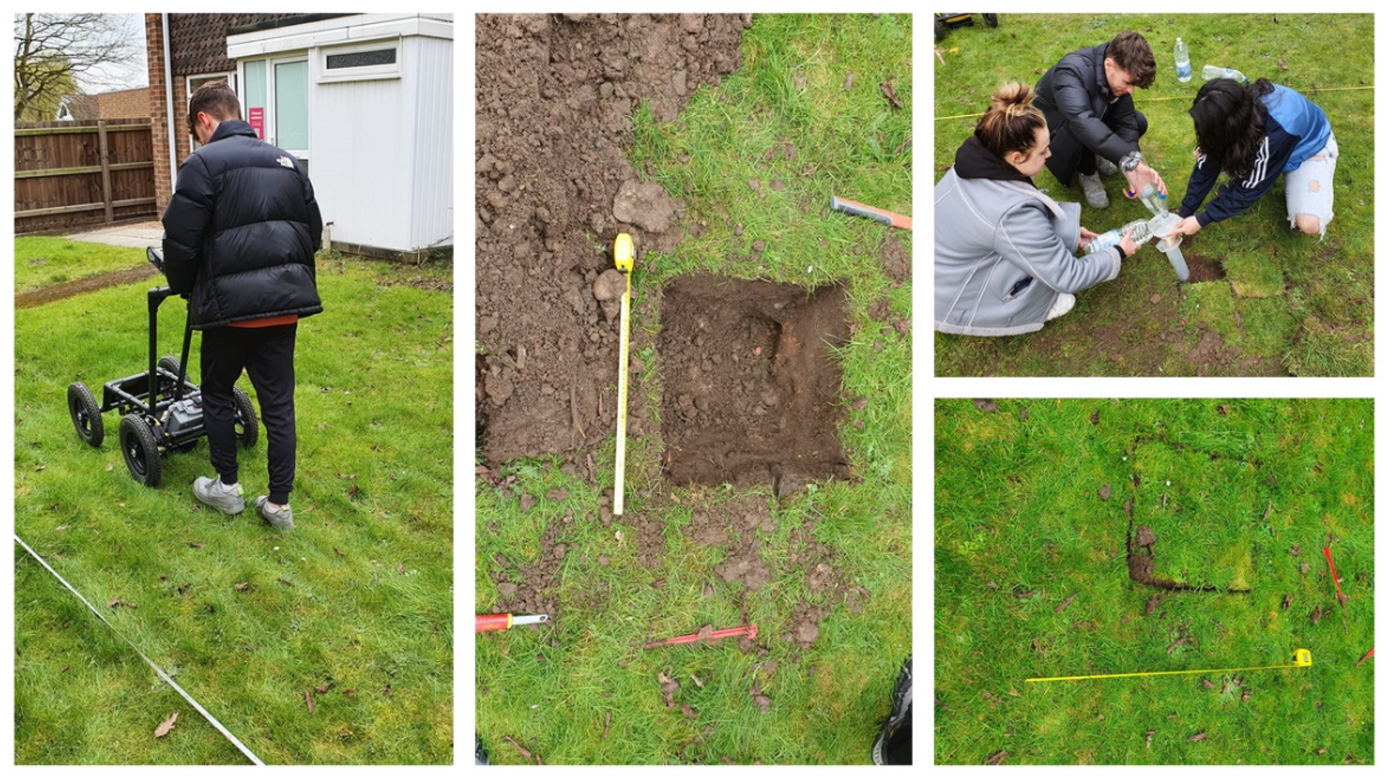
2. Materials and Methods

The burial site was created in the front garden of the Crime Scene House Facility (CSHF) at Nottingham Trent University, simulating ¼ of a real human burial at a crime scene. Therefore, the size of the burial in this experiment was 0.50 × 0.50 × 0.50 m3 (Figure 1).
Subsequently, it was necessary to determine the concentration of the NaCl dissolved in the water to simulate the body fluids at the same relative permittivity at 500 MHz. A literature review [44] on the effect of salinity on the dielectric properties of water, as well as an interim report on the compilation of the dielectric properties of body tissues at Rf and microwave frequencies [45], determines that the body fluids’ permittivity (ε) at 500 MHz is approximately 68, with an average conductivity of 3–5 S/m [46,47]. In this experiment, it is required to use the assumption of 5 S/m. From this, the Total Dissolved Solids (TDS) in parts per million was calculated [48]:
32,000 TDS, parts per million, 640 scale [TDS₆₄₀] = 5 S/m
This, in turn, can be converted to g/L using the calculation [49]:
1 g/L = 1000 ppm
Therefore, the concentration required of the saltwater was 32 g/L, and this was simulated in the subsurface.
Ten liters of this saline water were poured into the ground to match the size of the simulated grave. As the grave was dug to simulate ¼ of the size of a real human burial, being consistent with the simulation was important. Therefore, the formulas of Hume–Weyer and Watson were used to calculate the amount of body fluids in a male body with the dimensions of 170 cm height and 70 kg weight at 40 years old.
Hume–Weyer Formula [50]:
Male TBW = (0.194786 × 170) + (0.296785 × 70) − 14.012934 = 39.875636 = 39.9 L
Watson Formula [51]:
Male TBW = 2.447 − (0.09156 × 40) + (0.1074 × 170) + (0.3362 × 70) = 40.5766 = 40.6 L
The average of these calculations determined that a male of this stature contained 40.25 L of body fluids, which was simplified to 40 L to find the nearest integer.
Satellite imagery (using SkyWatch 4-bands satellite at 0.5 m resolution), UAV imagery (using MiniMavic, DJI), and GPR data, before and after the dig, were used to compare the results of the three RS methods and analyze the detectability of the anomaly due to the burial and the simulated decomposition fluids. With the satellite images, NDVI was utilized, whilst VARI was used with the UAV images. Both results were associated with the GPR data from the subsurface. The GPR was a Noggin SmartCart bistatic system from Sensors & Software, Inc., equipped with 500-MHz antennas.
The GPR measurements were performed following the Y-axis direction within a 3 × 4 m2 grid. There was a collection of 12 parallel lines with an interline of 0.25 m and a stacking of 4. Data were generally of good quality, and only the standard DME (Dewow + Envelope + Migration) migration at an average velocity of 0.11 m/ns was necessary.
The experiment ran for 36 days, and the data were collected following the schedule in Table 1. Due to the nature of this initial experiment, although the weather during the 36 days had been mostly rainfall-free, here, we chose not to consider the influence of rain but focused only on the effect of simulated body fluids in a specific area.

3. Results and Discussion
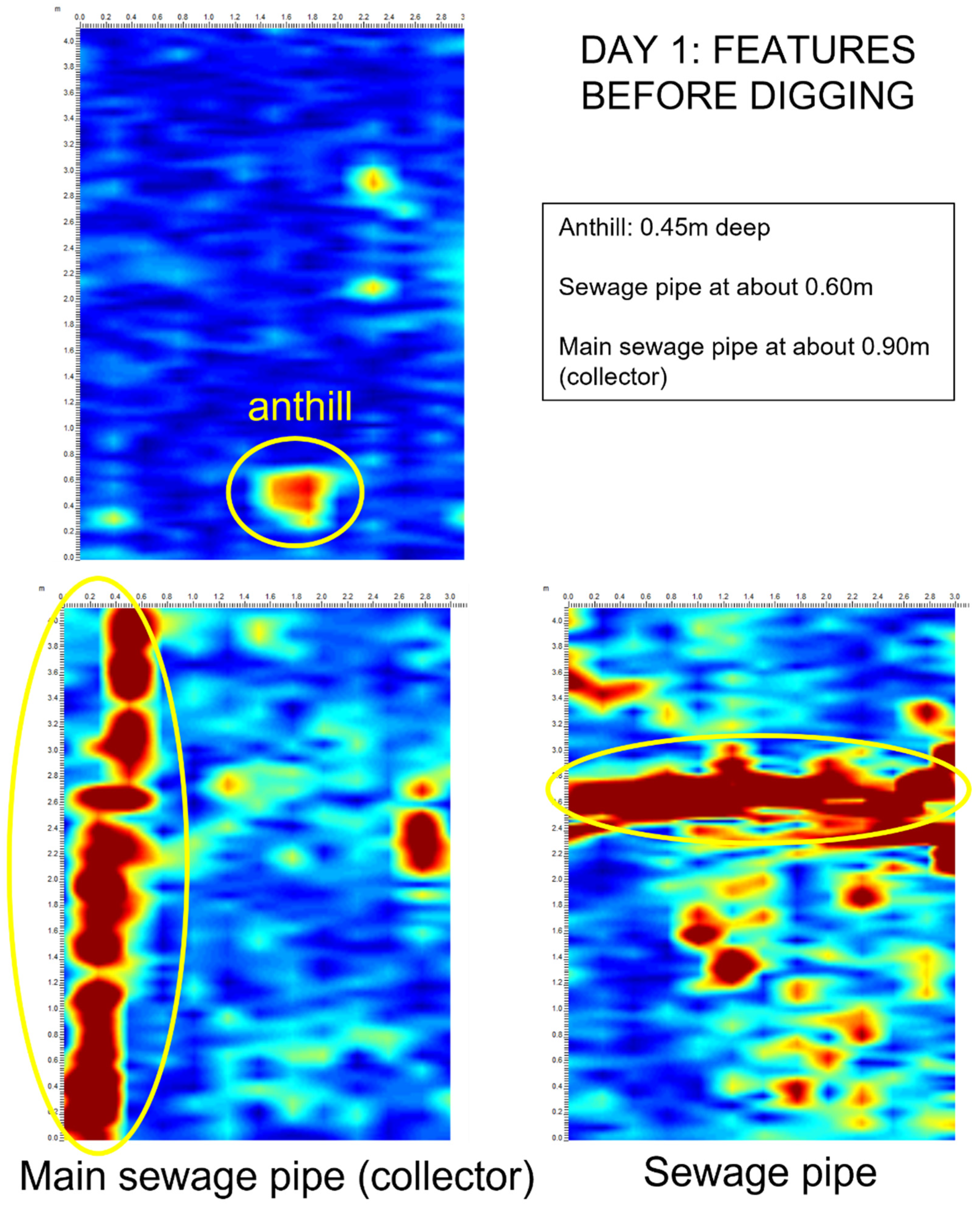
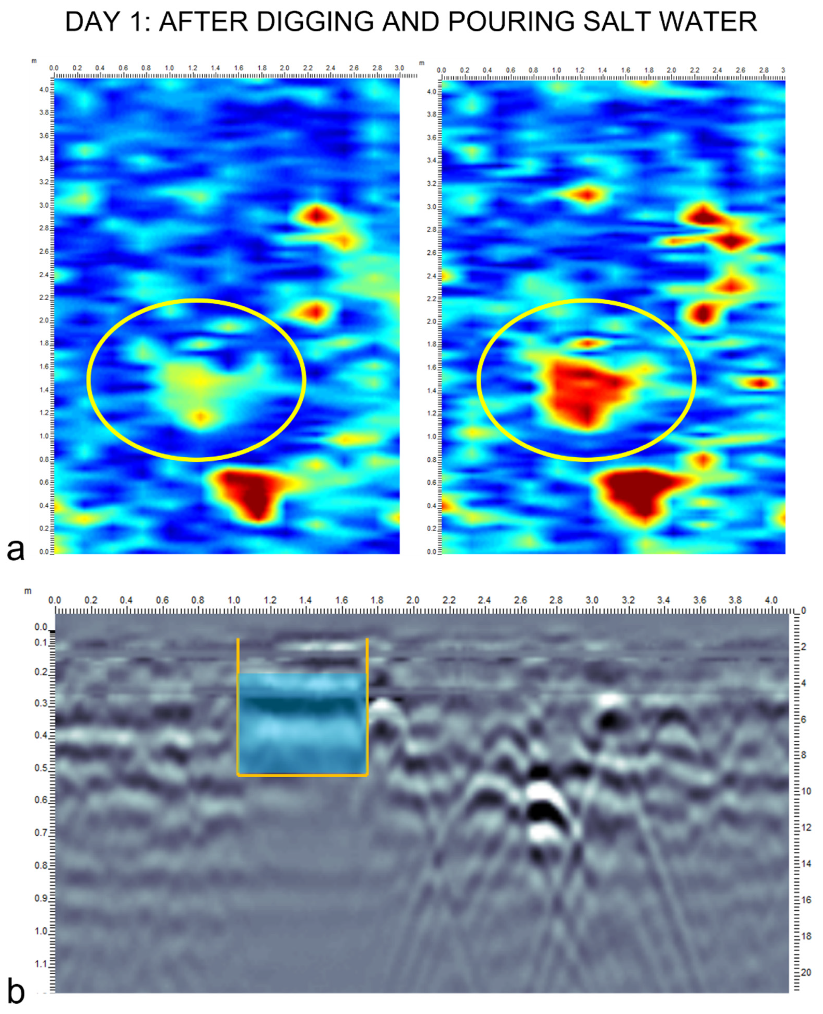
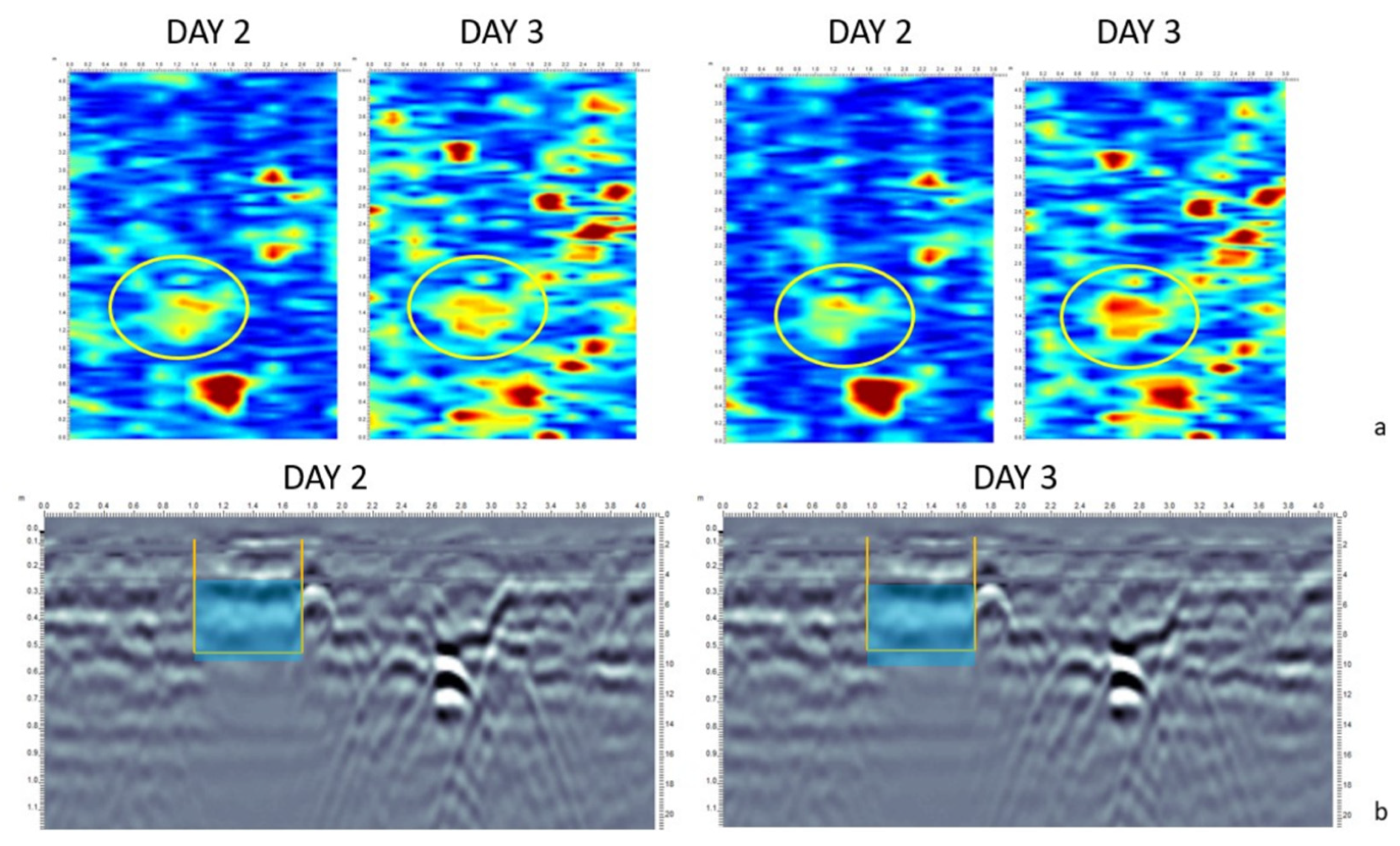
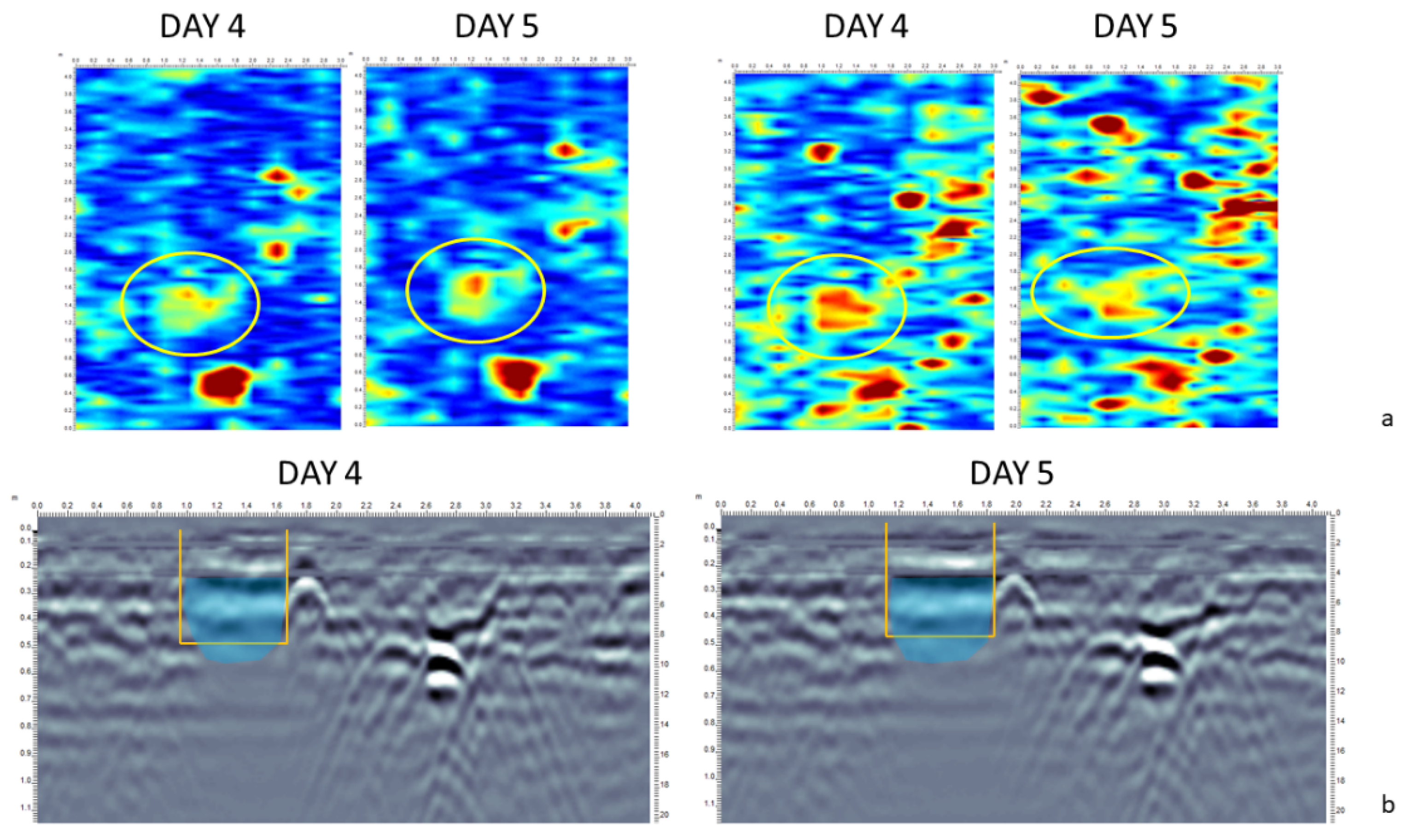
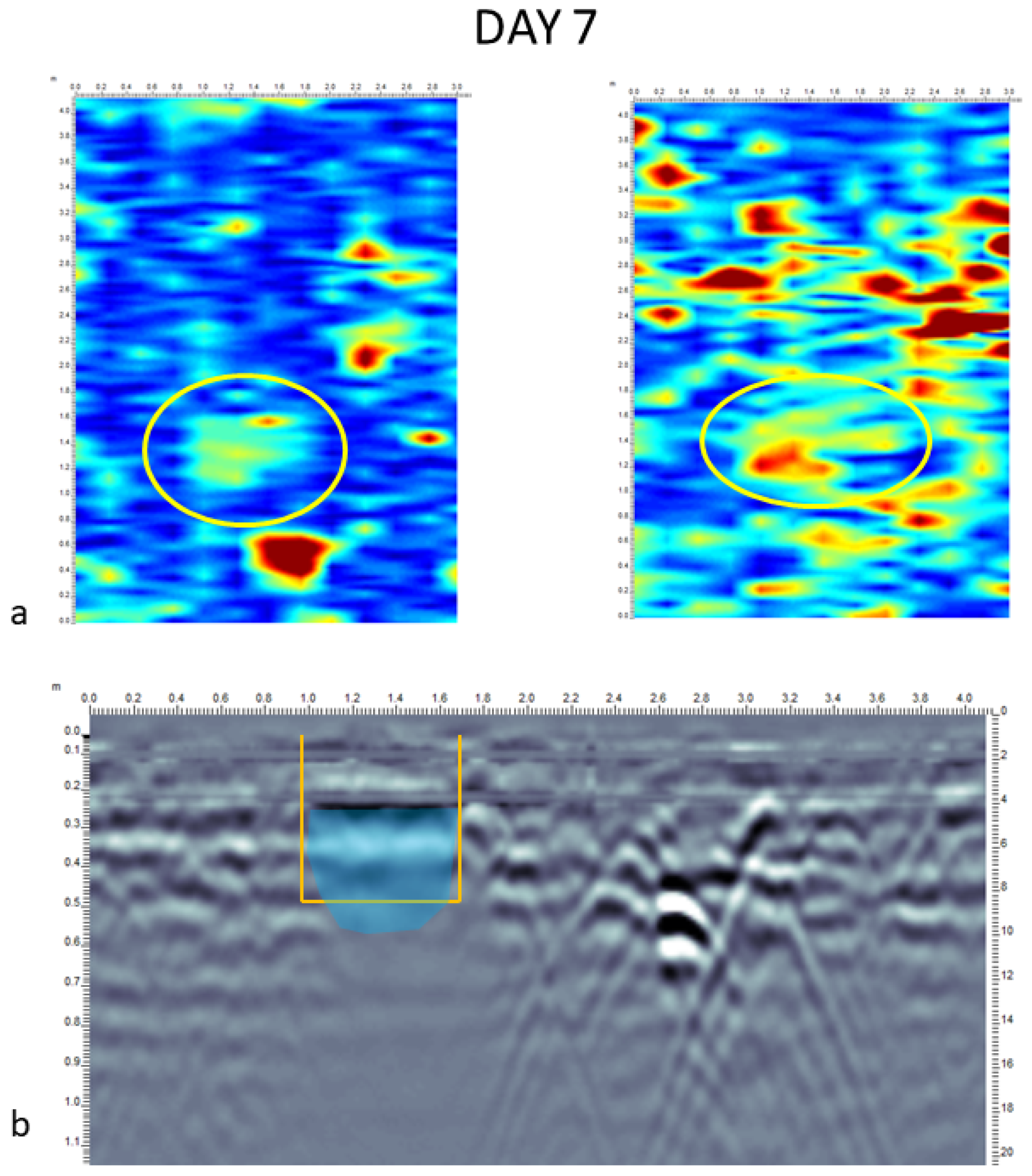
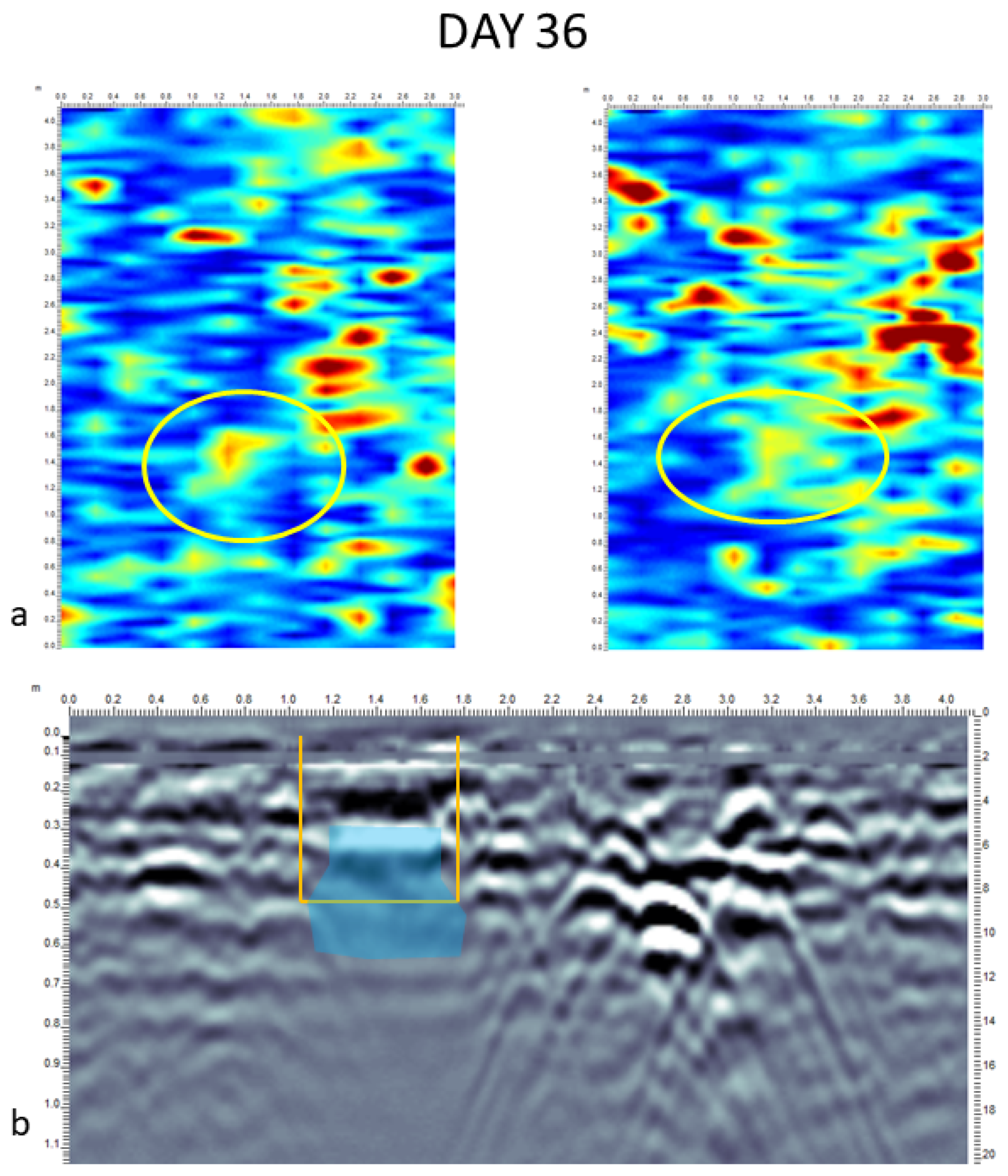
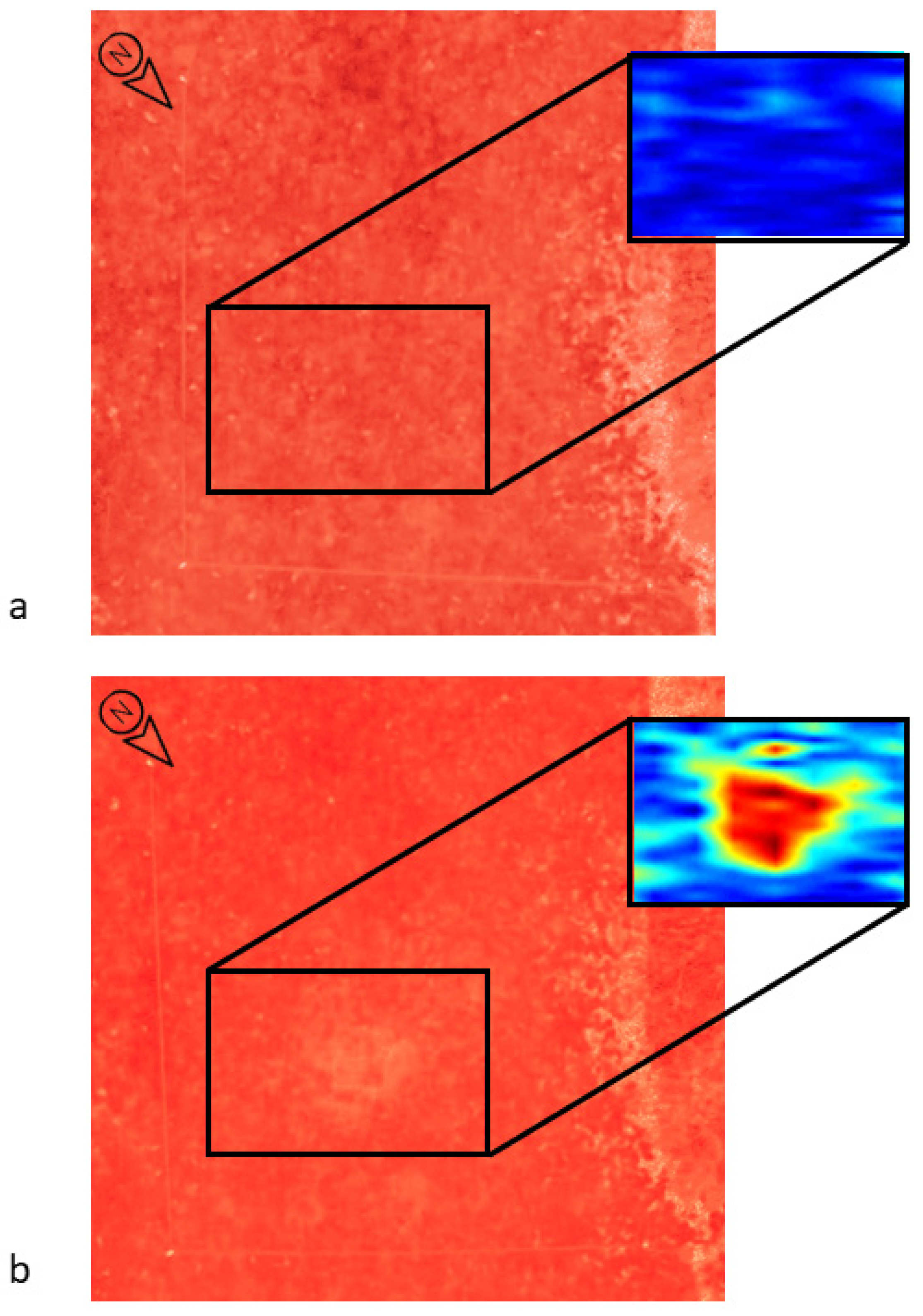
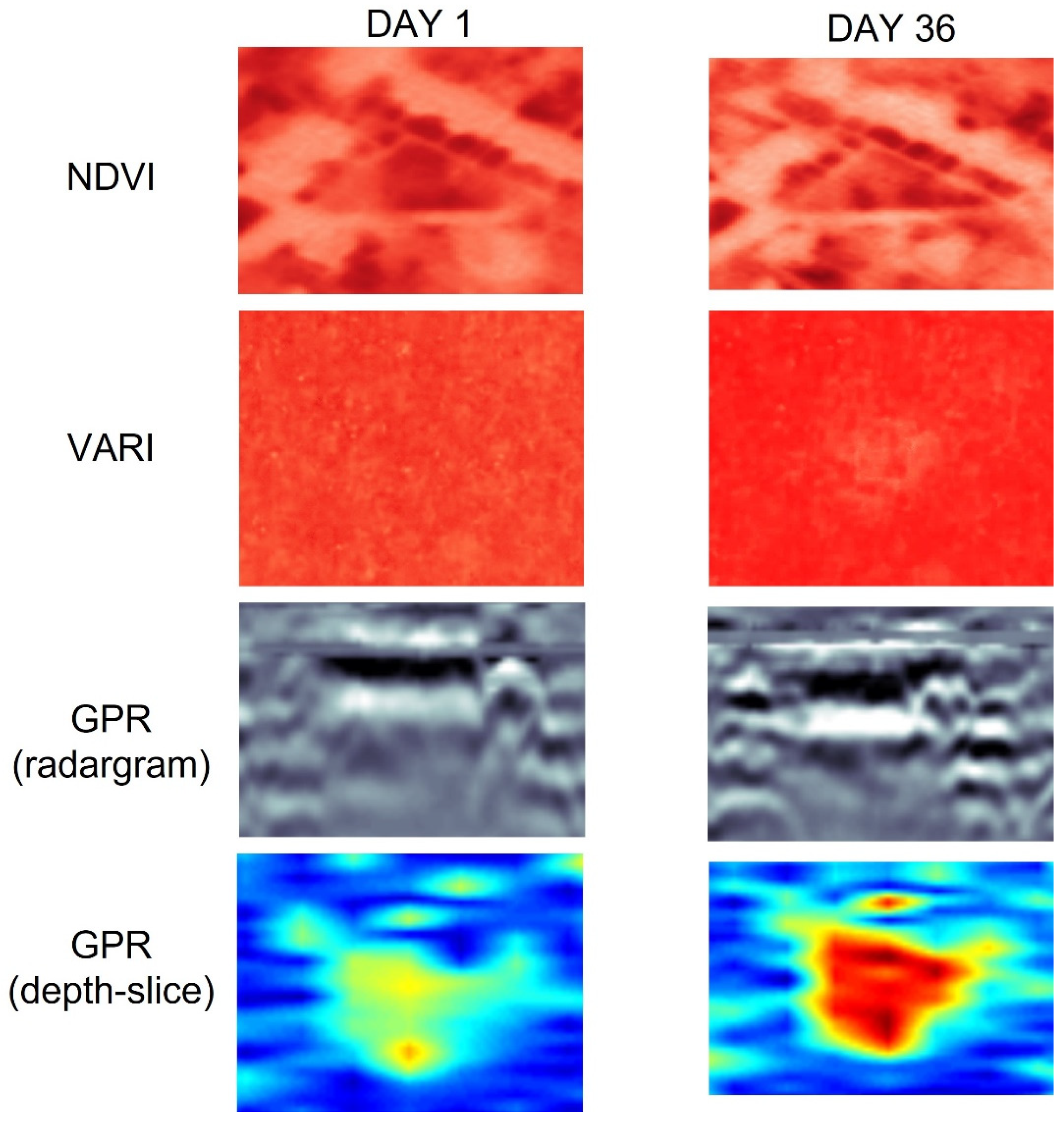
3.1. GPR Results

The initial GPR analysis of the subsurface aimed to detect both the initial constant dielectric of the soil and possible buried features before starting the experiment to exclude them from the next analyses.
Due to clay soil, the initial dielectric constant was 7. In addition, the GPR depth slices of this initial scan showed three possible disturbances in the subsurface. At the shallowest depth, an anthill can be seen at 0.45 m deep. The other two most prominent features of this GPR scan were two possible sewage pipes coming out of the property on the north-western side of the garden. The first sewage pipe crossed the grid in the NW-SE direction at a depth of about 0.60 m. The second sewage pipe was a collector pipe, located at a slightly lower depth of about 0.90 m, and ran perpendicular to the previous one (Figure 2). Based on these preliminary results, it was possible to not only understand the buried features before the experiment but also determine where exactly to dig without any interference.
After this preliminary geophysical investigation, the GPR data were collected according to the schedule in Table 1 to observe the migration of the simulated body fluids.
On the first day, after pouring the liquid and properly refilling the grave, between 1.25 and 1.55 m along the Y-axis and between 0.85 and 1.60 m along the X-axis, the GPR radargram detected a characteristic anomaly due to the burial geometry (two soil cuts and the refilling) [10] (Figure 3a). Inside this anomaly, at 0.30 m deep, the GPR radargram also highlights a strong horizontal anomaly due to the presence of the simulated body fluids. The depth slices between 0.20 m (top) and 0.50 m (bottom) confirmed the moist anomaly and helped to understand the preliminary geometry of the liquids at the beginning of the experiment (Figure 3b). This proved relevant to better understanding the movement and migration of the simulated body fluids during the following days.
On the second and third day, the GPR results showed the presence of both the burial and the fluids, similarly to the first day. Notably, the fluids started to migrate toward gravity, and consequently, the relative anomaly in both the radargram and the depth slices moved downward by a few centimeters, between 0.25/0.27 m (top) and 0.55/0.58 m (bottom) deep (Figure 4a,b).
On the fourth and fifth day, both GPR radargrams and depth slices again showed anomalies due to both the burial and the fluids. In Figure 5, it is possible to see how the moist anomaly is slowly progressing downward due to gravity (0.30 m for the top and 0.60 m for the bottom) and tending to spread at the bottom, making the geometry of the fluid anomaly less evident.
On the seventh day, the GPR data were showing more evidently the trend noticed on the fourth and the fifth days. The fluids’ migration due to gravity has stopped (0.30 m for the top and 0.60 m for the bottom), but the fluids are spreading a bit more at the bottom and are less evident (Figure 6).
Finally, on the 36th day, both GPR radargrams and depth slices confirmed the abovementioned process in which the movement of the simulated body fluids is no more downward due to the gravity but is slightly lateral and spreading at a depth of about 0.60 m with a relative dispersion and reduction of the liquid in the surrounding layers without being able to well define its limits and geometry (Figure 7).
The progression of the simulated body fluids through the subsurface provides an abundance of information about how the fluids from a decomposing body would act in a real burial. The downward migration of the fluids was expected in the initial days of this experiment. However, the lateral movement was not expected so soon. Many factors must have influenced the migration of the fluids, such as the composition of the soil or the weather. To determine whether these factors influenced the results of this experiment, further experiments are needed.

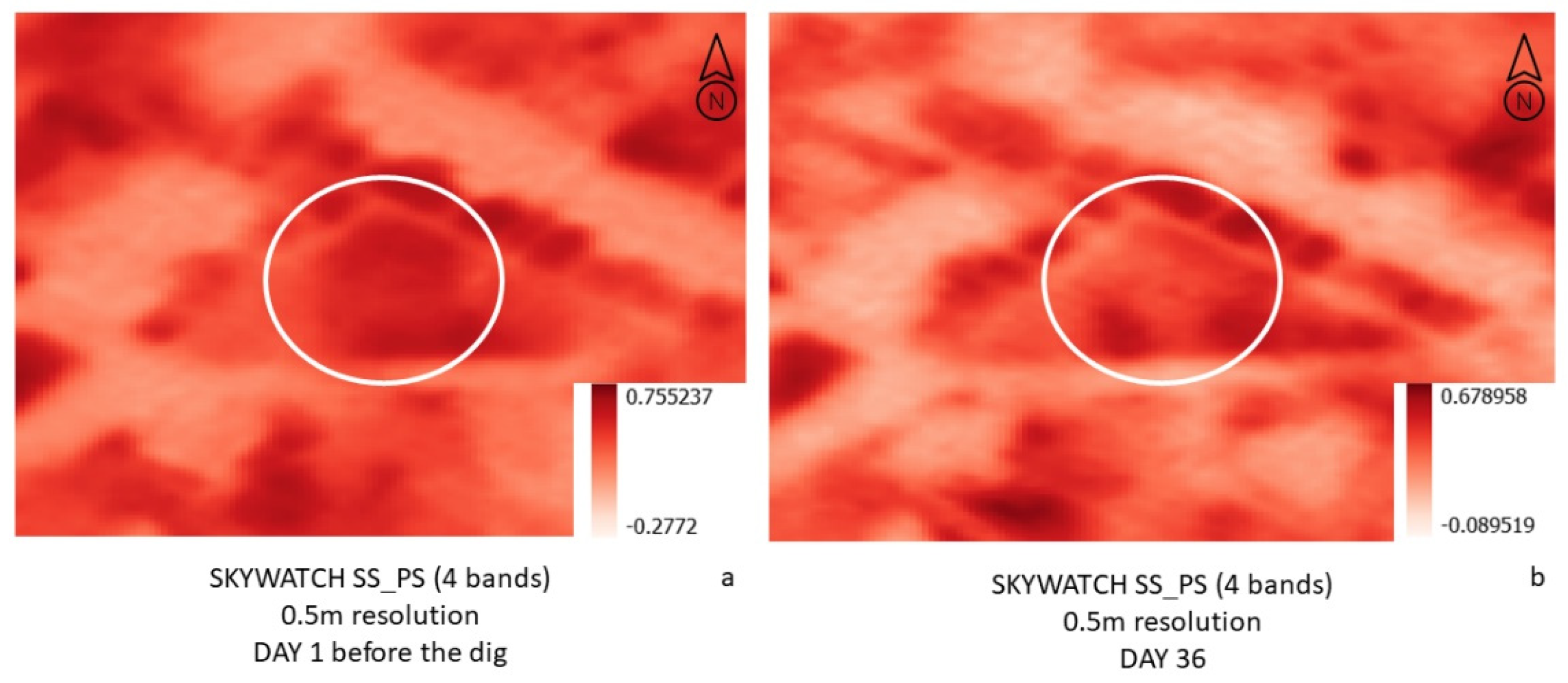
3.2. Satellite Imagery Using NDVI

For the aim of this research, it was possible to find satellite images with the abovementioned characteristics showing the vegetation index before and after the soil was disturbed. In real scenarios at crime scenes with buried bodies, forensic scientists cannot always get ahead of aerial images or any type of photos taken by crime scene investigators before the burial occurred, thus making satellite imagery a real advantage toward the case. NDVI can reveal all possible anomalies that can help determine when the body was buried in a specific location, providing an accurate estimation of the time period. Figure 8 shows the comparison between the satellite images taken before and after (day 36) the dig. Even if other satellite images were available (almost daily), it was decided to focus on the longest period to better highlight the relevance of the methodology simulating the extended period of an investigation.
By applying NDVI analysis to both images, quantifying the vegetation, and highlighting the relationship between near-infrared and red light, a pseudocolor difference was revealed between the two images. While Figure 8a shows the area before the dig, with no visible anomalies in the vegetation, Figure 8b shows the NDVI satellite image of the same area at the end of the experiment, showing a lighter shade of red, which indicates a difference in the vegetation. This difference is visible and mostly detectable by a comparison of the two images. However, the resolution (0.5 m) cannot appreciate very high details. For this reason, even if the NDVI method is valid, it must be a part of other measurements.

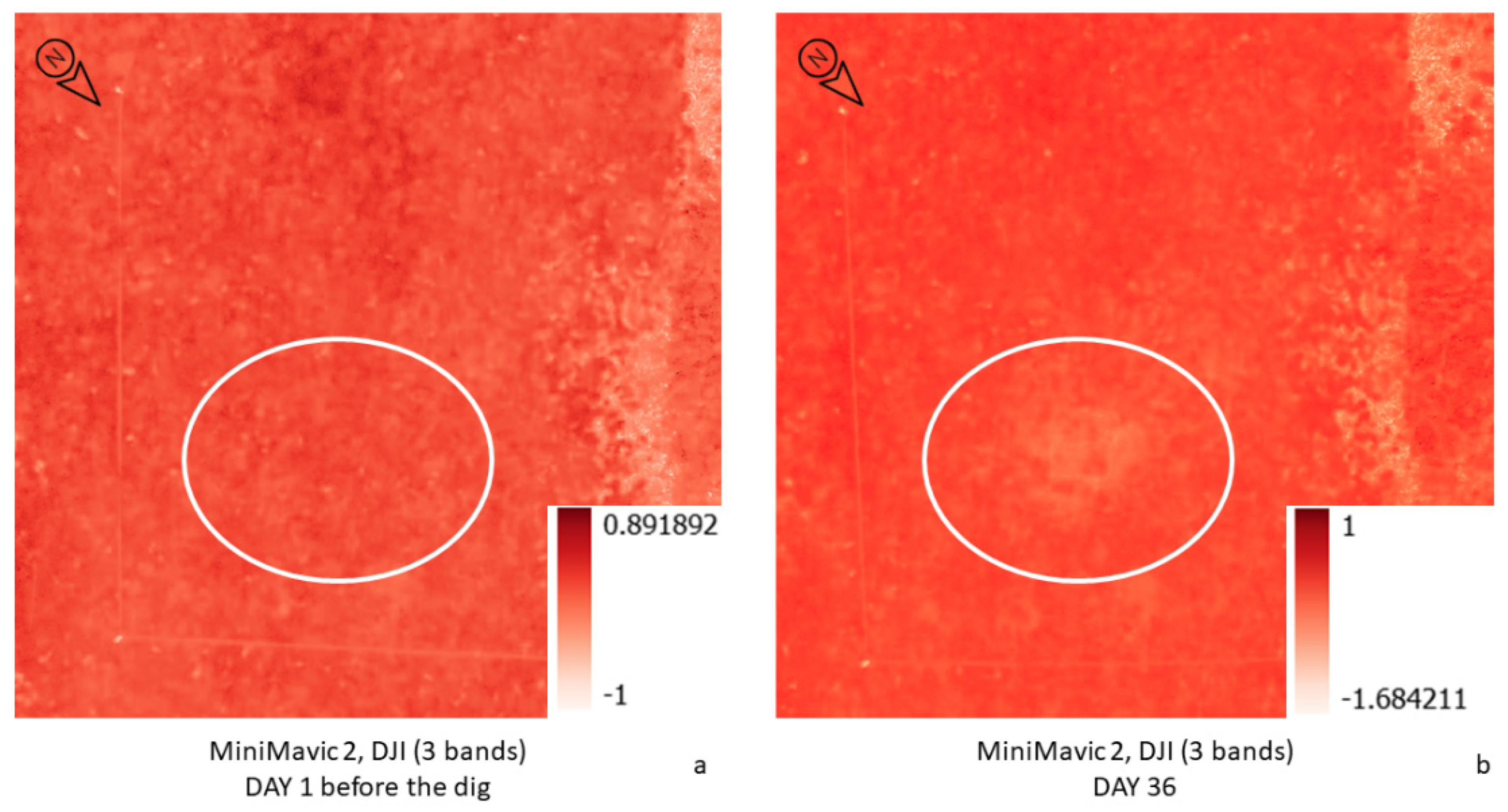
3.3. Drone Imagery Using VARI

Unlike in a real-life crime scene, during this experiment, it was possible to get UAV imagery before the dig to see if any anomalies were present in the area before the experimentation. When VARI was applied in pseudocolor, the only visible anomalies were in the bushes right next to the scene (Figure 9a). Once the dig was completed, the body fluids were poured in, and the excavation refilled the dig with the same lump of soil, aerial images using the UAV were collected every day of the experiment. Figure 9b shows the UAV image taken on day 36, right at the end of the experiment, with the application of VARI. Even if the UAV images were taken throughout the whole experiment period, it was decided to be consistent with the options taken with the satellite imagery.
The UAV imagery is very high resolution, and the significance of the detected anomaly allows a clear interpretation of the data. While the aerial images of a crime scene are not always available before the concealment is committed, this VARI method, using simple RGB images, demonstrates tremendous potential for research and exploration.

3.4. Limitations and Future Perspectives

The data recorded in this preliminary research were mainly focused on the simulated body fluids’ detectability by the GPR to assist the investigations at crime scenes involving potential clandestine graves and geophysical searches. This was the main reason why the dielectric constant of the body fluids was chosen for the simulation. Although the simulation of the body fluids related to the dielectric constant was accurate and allowed a valid experiment to be conducted, other typical characteristics of the body fluids, such as viscosity and density, were left out and would be studied in future simulations. Moreover, the effect of external factors like rainfall and scavengers was also taken relatively into consideration, and, in the future, this will be included in a more substantial and wide-ranging experiment. In addition, we are aware that this experiment focuses on only one soil type. Therefore, given the success of this preliminary experiment, the next step will be to consider increasing the case study by subjecting different soil types such as sandy, silty, limestone, etc., to a similar experiment and evaluating the relative outcomes. Further simulations will also take into consideration other burial alternatives, like carbonized bodies, mass graves, buried bodies wearing clothes, etc.
Nevertheless, the experiment showed how other RS methods supported the aim. Figure 10 shows the GPR maps before and after the dig, georeferenced at the site, and compared to the equivalent VARI images.
This research will help law enforcement determine the location of any potential burials by detecting the movement of the body fluids in the subsurface. It could also help in a situation where a corpse has been moved from a certain location, and the location still has body fluids that can be detected in the subsurface. This could provide vital evidence to the court that could result in assisting the prosecution of the culprit. It should be noted, however, that the volume of body fluids the NDVI and VARI analyses identified quite clearly in the subsurface is not so much as that in a burial. Moreover, as pointed out earlier, based on the different resolutions, VARI reported more favorable results (Figure 11).
Moreover, the potential for a full-sized burial could be explored, as this project was scaled down to a quarter of a full-sized burial due to restraints that were out of our control. A full-scale burial could provide more accurate results due to the larger volume of the body fluids. The methods in this experiment were consistent, as we scaled down everything to a quarter of the size. However, using a full-scale burial may yield further results that were not evident in this experiment.

4. Conclusions

This research project aimed to find and investigate geoscientific methods that are non-destructive to the crime scene and establish how they can assist a criminal investigation and help law enforcement to map and locate suspicious burials.
The potential offered by the RS methods is remarkable if we consider the relative ease of obtaining any kind of information from these methods because of the short time and distance involved with them. This can be repeated over time or, in some cases, almost continuously with greater spatial coverage, objectivity, precision, and overall cost-effectiveness when compared to the conventional detection methods. Therefore, RS can represent a real revolution in the field of constant monitoring and is, in fact, already a reality that has been established for some time with increasing applications and diffusion. Thus, it is obvious how these methods play a fundamental role in better understanding the forensic evolution of specific crime scenes [52].
Despite the limitations mentioned earlier, strictly related to the preliminary nature of it, this first-step experiment helped to better understand how decomposition in the subsurface does not always migrate in the way that was initially expected (toward gravity), and several factors need to be considered.
Thanks to the continuous improvement of RS systems, the possibilities of its application and use are always increasing with more detail and precision. It is clear how this result leads to a different thinking of the forensic archaeological context in general and forensic excavation in particular. This amount of RS information can easily help save money, time, and human resources to provide a more accurate ground-truthing.
Finally, the ethical aspect is also not to be underestimated in this research. It has been shown that with proper care, simulating a burial with decomposition fluids is possible even without using pig carcasses. This discussion is timely and has several researchers on the front lines [53]. For the future, it is hoped that this paper will not only provide insights to improve crime scene forensic investigations but also, and more importantly, enable a more ethical and sustainable alternative approach within forensic science.

Author Contributions

Conceptualization, P.M.B., D.M., A.M., N.K. and M.M.; methodology, P.M.B.; software, P.M.B.; validation, P.M.B.; formal analysis, P.M.B., D.M., A.M., N.K. and M.M.; investigation, P.M.B., D.M., A.M., N.K. and M.M.; resources, P.M.B.; data curation, P.M.B., D.M., A.M., N.K. and M.M.; writing—original draft preparation, P.M.B., D.M., A.M., N.K. and M.M.; writing—review and editing, P.M.B., D.M., A.M., N.K. and M.M.; visualization, P.M.B., D.M., A.M., N.K. and M.M.; supervision, P.M.B.; project administration, P.M.B. All authors have read and agreed to the published version of the manuscript.

Funding

This research received no external funding.

Informed Consent Statement

Not applicable.

Conflicts of Interest

The authors declare no conflict of interest.

References

  1. Elmes, G.A.; Roedl, G.; Conley, J. (Eds.) Forensic GIS: The Role of Geospatial Technologies for Investigating Crime and Providing Evidence; Geotechnologies and the Environment; Springer: Dordrecht, The Netherlands, 2014; ISBN 978-94-017-8756-7. [Google Scholar]
  2. Avery, T.E. Fundamentals of Remote Sensing and Airphoto Interpretation/Thomas Eugene Avery, Graydon Lennis Berlin, 15th ed.; Prentice Hall: Upper Saddle River, NJ, USA, 1992; ISBN 978-0-02-305035-0. [Google Scholar]
  3. Hodge, S. Satellite Data and Environmental Law: Technology Ripe for Litigation Application. Pace Environ. Law Rev. 1997, 14, 691. [Google Scholar]
  4. Barone, P.; Di Maggio, R.M. Low-Cost CSI Using Forensic GPR, 3D Reconstruction, and GIS. J. Geogr. Inf. Syst. 2019, 11, 493–499. [Google Scholar] [CrossRef]
  5. Rocke, B.; Ruffell, A. Detection of Single Burials Using Multispectral Drone Data: Three Case Studies. Forensic Sci. 2022, 2, 6. [Google Scholar] [CrossRef]
  6. Pensieri, M.G.; Garau, M.; Barone, P.M. Drones as an Integral Part of Remote Sensing Technologies to Help Missing People. Drones 2020, 4, 15. [Google Scholar] [CrossRef]
  7. Rocke, B.; Ruffell, A.; Donnelly, L. Drone Aerial Imagery for the Simulation of a Neonate Burial Based on the Geoforensic Search Strategy (GSS). J. Forensic Sci. 2021, 66, 1506–1519. [Google Scholar] [CrossRef]
  8. Hildmann, H.; Kovacs, E. Review: Using Unmanned Aerial Vehicles (UAVs) as Mobile Sensing Platforms (MSPs) for Disaster Response, Civil Security and Public Safety. Drones 2019, 3, 59. [Google Scholar] [CrossRef]
  9. Barone, P.M. Understanding Buried Anomalies: A Practical Guide to GPR; LAP LAMBERT Academic Publishing: Saarbrücken, Germany, 2016. [Google Scholar]
  10. Barone, P.M. Forensic Geophysics. In Geoscientists at Crime Scenes: A Companion to Forensic Geoscience; Di Maggio, R.M., Barone, P.M., Eds.; Soil Forensics; Springer International Publishing: Cham, Germany, 2017; pp. 175–190. ISBN 978-3-319-58048-7. [Google Scholar]
  11. Ruffell, A.; McKinley, J. Geoforensics|Wiley. Available online: https://www.wiley.com/en-us/Geoforensics-p-9780470057353 (accessed on 24 June 2022).
  12. Schultz, J.J. Using Ground-Penetrating Radar to Locate Clandestine Graves of Homicide Victims: Forming Forensic Archaeology Partnerships With Law Enforcement. Homicide Stud. 2007, 11, 15–29. [Google Scholar] [CrossRef]
  13. Leblanc, G.; Kalacska, M.; Soffer, R. Detection of Single Graves by Airborne Hyperspectral Imaging. Forensic Sci. Int. 2014, 245, 17–23. [Google Scholar] [CrossRef]
  14. Parrott, E.; Panter, H.; Morrissey, J.; Bezombes, F. A Low Cost Approach to Disturbed Soil Detection Using Low Altitude Digital Imagery from an Unmanned Aerial Vehicle. Drones 2019, 3, 50. [Google Scholar] [CrossRef]
  15. Wueste, E.; Facchin, G.; Barone, P.M. Aventinus Minor Project: Remote Sensing for Archaeological Research in Rome (Italy). Remote Sens. 2022, 14, 959. [Google Scholar] [CrossRef]
  16. Meeragandhi, G.; Arun, S.P.; Thummala, N.; Christy, A. Ndvi: Vegetation Change Detection Using Remote Sensing and Gis—A Case Study of Vellore District. Procedia Comput. Sci. 2015, 57, 1199–1210. [Google Scholar] [CrossRef] [Green Version]
  17. Makario, S. Normalized Difference Vegetation Index (NDVI) in Remote Sensing. Available online: https://blog.heptanalytics.com/normalized-difference-vegetation-indexndvi-in-remote-sensing/ (accessed on 24 June 2022).
  18. Weier, J.; Herring, D. Measuring Vegetation (NDVI & EVI). Available online: https://earthobservatory.nasa.gov/features/MeasuringVegetation (accessed on 9 November 2021).
  19. Brown, J. NDVI, the Foundation for Remote Sensing Phenology|U.S. Geological Survey. Available online: https://www.usgs.gov/special-topics/remote-sensing-phenology/science/ndvi-foundation-remote-sensing-phenology?msclkid=0601ef9faf6611ecafe6714da26ff426 (accessed on 24 June 2022).
  20. Lasaponara, R.; Masini, N. Identification of Archaeological Buried Remains Based on the Normalized Difference Vegetation Index (NDVI) from QuickBird Satellite Data. Geosci. Remote Sens. Lett. IEEE 2006, 3, 325–328. [Google Scholar] [CrossRef]
  21. Donnelly, L.; Harrison, M. Geomorphological and Geoforensic Interpretation of Maps, Aerial Imagery, Conditions of Diggability and the Colour-Coded RAG Prioritization System in Searches for Criminal Burials. Geol. Soc. Lond. Spec. Publ. 2013, 384, 173–194. [Google Scholar] [CrossRef]
  22. Donnelly, L.; Harrison, M. Geoforensic search strategy (GSS): Ground searches related to homicide graves, counterterrorism and serious crime. In A guide to Forensic Geology; Donnelly, L.J., Pirrie, D., Harrison, M., Ruffell, A., Dawson, L., Eds.; Geological Society: London, UK, 2021; pp. 21–85. [Google Scholar] [CrossRef]
  23. Harrison, M.; Donnelly, L.J. Locating Concealed Homicide Victims: Developing the Role of Geoforensics. In Criminal and Environmental Soil Forensics; Ritz, K., Dawson, L., Miller, D., Eds.; Springer: Dordrecht, The Netherlands, 2009; pp. 197–219. ISBN 978-1-4020-9204-6. [Google Scholar]
  24. Lindsey, A.J.; Craft, J.C.; Barker, D.J. Modeling Canopy Senescence to Calculate Soybean Maturity Date Using NDVI. Crop Sci. 2020, 60, 172–180. [Google Scholar] [CrossRef]
  25. Limongiello, M.; Gujski, L.; De Vita, C. Analysis of RGB Images to Enhance Archaeological Cropmark Detection: The Case Study of Nuceriola, Italy. In Proceedings of the 42th International Conference of Representation Disciplines Teachers Congress of Unione Italiana per il Disegno; Franco Angeli: Milan, Italy, 2020; pp. 2360–2368. [Google Scholar] [CrossRef]
  26. Ronchi, D.; Limongiello, M.; Barba, S. Correlation among Earthwork and Cropmark Anomalies within Archaeological Landscape Investigation by Using LiDAR and Multispectral Technologies from UAV. Drones 2020, 4, 72. [Google Scholar] [CrossRef]
  27. Pringle, J.K.; Stimpson, I.G.; Wisniewski, K.D.; Heaton, V.; Davenward, B.; Mirosch, N.; Spencer, F.; Jervis, J.R. Geophysical Monitoring of Simulated Clandestine Burials of Murder Victims to Aid Forensic Investigators. Geol. Today 2021, 37, 63–65. [Google Scholar] [CrossRef]
  28. Pringle, J.K.; Jervis, J.; Cassella, J.P.; Cassidy, N.J. Time-Lapse Geophysical Investigations over a Simulated Urban Clandestine Grave. J. Forensic Sci. 2008, 53, 1405–1416. [Google Scholar] [CrossRef]
  29. Ruffell, A.; Mckinley, J.; Donnelly, L.; Harrison, M.; Keaney, A. Geoforensics, 1st ed.; John Wiley & Sons Inc: Chichester, UK; Hoboken, NJ, USA, 2008; ISBN 978-0-470-05735-3. [Google Scholar]
  30. Koppenjan, S.K.; Nevada, B.; Schultz, J.J.; Falsetti, A.B.; Collins, M.E.; Ono, S.; Lee, H. The Application of GPR in Florida for Detecting Forensic Burials. In Proceedings of the 16th EEGS Symposium on the Application of Geophysics to Engineering and Environmental Problems (SAGEEP), San Antonio, TX, USA, 6–10 April 2003; p. 190-00063. [Google Scholar] [CrossRef]
  31. Midi, N.S.; Sasaki, K.; Ohyama, R.; Shinyashiki, N. Broadband Complex Dielectric Constants of Water and Sodium Chloride Aqueous Solutions with Different DC Conductivities. IEEJ Trans. Electr. Electron. Eng. 2014, 9, S8–S12. [Google Scholar] [CrossRef]
  32. Persico, R. Introduction to Ground Penetrating Radar: Inverse Scattering and Data Processing; IEEE: Hoboken, NJ, USA, 2014; ISBN 978-1-118-30500-3. [Google Scholar]
  33. Jol, H.M. Ground Penetrating Radar Theory and Applications; Elsevier: Amsterdam, The Netherlands, 2009. [Google Scholar]
  34. Conyers, L.B. Ground-Penetrating Radar. In Encyclopedia of Geoarchaeology; Gilbert, A.S., Ed.; Springer: Dordrecht, The Netherlands, 2017; pp. 367–378. ISBN 978-1-4020-4409-0. [Google Scholar]
  35. Donnelly, L.J.; Pirrie, D.; Harrison, M.; Ruffell, A.; Dawson, L.A. The Geological Society of London—A Guide to Forensic Geology; GSL Miscellaneous Titles; GSL: London, UK, 2021; ISBN 978-1-78620-488-2. [Google Scholar]
  36. Barone, P.M.; Ferrara, C.; Pettinelli, E.; Fazzari, A. Forensic Geophysics: How the GPR Technique Can Help with Forensic Investigations. In Proceedings of the Soil in Criminal and Environmental Forensics; Kars, H., van den Eijkel, L., Eds.; Springer International Publishing: Cham, Switzerland, 2016; pp. 213–227. [Google Scholar]
  37. Barone, P.M.; Ferrara, C.; Pettinelli, E.; Annan, A.P.; Fazzari, A.; Redman, D. Forensic Geophysics: How GPR Could Help Police Investigations. In Proceedings of the Near Surface Geoscience 2012—18th European Meeting of Environmental and Engineering Geophysics; Paris, France, 3–5 September 2012, European Association of Geoscientists & Engineers: Houten, The Netherlands, 2012; p. 306-00001. [Google Scholar] [CrossRef]
  38. Barone, P.M.; Di Maggio, R.M. Forensic Geophysics: Ground Penetrating Radar (GPR) Techniques and Missing Persons Investigations. Forensic Sci. Res. 2019, 4, 337–340. [Google Scholar] [CrossRef]
  39. Solla, M.; Riveiro, B.; Álvarez Cid, M.; Arias, P. Experimental Forensic Scenes for the Characterization of Ground-Penetrating Radar Wave Response. Forensic Sci. Int. 2012, 220, 50–58. [Google Scholar] [CrossRef]
  40. Di Maggio, R.M.; Barone, P.M. (Eds.) Geoscientists at Crime Scenes: A Companion to Forensic Geoscience; Soil Forensics; Springer International Publishing: Berlin/Heidelberg, Germany, 2017; ISBN 978-3-319-58047-0. [Google Scholar]
  41. Collins, S.; Maestrini, L.; Ueland, M.; Stuart, B. A Preliminary Investigation to Determine the Suitability of Pigs as Human Analogues for Post-Mortem Lipid Analysis. Talanta Open 2022, 5, 100100. [Google Scholar] [CrossRef]
  42. DeBruyn, J.M.; Hoeland, K.M.; Taylor, L.S.; Stevens, J.D.; Moats, M.A.; Bandopadhyay, S.; Dearth, S.P.; Castro, H.F.; Hewitt, K.K.; Campagna, S.R.; et al. Comparative Decomposition of Humans and Pigs: Soil Biogeochemistry, Microbial Activity and Metabolomic Profiles. Front. Microbiol. 2021, 11, 608856. [Google Scholar] [CrossRef] [PubMed]
  43. Matuszewski, S.; Hall, M.J.R.; Moreau, G.; Schoenly, K.G.; Tarone, A.M.; Villet, M.H. Pigs vs People: The Use of Pigs as Analogues for Humans in Forensic Entomology and Taphonomy Research. Int. J. Legal Med. 2020, 134, 793–810. [Google Scholar] [CrossRef] [PubMed]
  44. Corwin, D.; Yemoto, K. Salinity: Electrical Conductivity and Total Dissolved Solids. Soil Sci. Soc. Am. J. 2020, 84, 1442–1461. [Google Scholar] [CrossRef]
  45. Gadani, D.; Rana, V.; Bhatnagar, S.; Prajapati, A.; Vyas, A.D. Effect of Salinity on the Dielectric Properties of Water. Indian J. Pure Appl. Phys. 2012, 50, 405–410. [Google Scholar]
  46. Klemetsen, Ø. Design and Evaluation of a Medical Microwave Radiometer for Observing Temperature Gradients Subcutaneously in the Human Body. Ph.D. Thesis, University of Tromsø, Tromsø, Norway, 2012. [Google Scholar]
  47. Andreuccetti, D.; Fossi, R.; Petrucci, C. An Internet Resource for the Calculation of the Dielectric Properties of Body Tissues in the Frequency Range 10 Hz–100 GHz. Available online: http://niremf.ifac.cnr.it/tissprop/ (accessed on 24 June 2022).
  48. Rusydi, A.F. Correlation between Conductivity and Total Dissolved Solid in Various Type of Water: A Review. IOP Conf. Ser. Earth Environ. Sci. 2018, 118, 012019. [Google Scholar] [CrossRef]
  49. Petrucci, R.H.; Harwood, W.S.; Herring, G. General Chemistry: Principles and Modern Applications, 11th ed.; Pearson: Toronto, ON, Canada, 2017. [Google Scholar]
  50. Hume, R.; Weyers, E. Relationship between Total Body Water and Surface Area in Normal and Obese Subjects. J. Clin. Pathol. 1971, 24, 234–238. [Google Scholar] [CrossRef]
  51. Watson, P.E.; Watson, I.D.; Batt, R.D. Total Body Water Volumes for Adult Males and Females Estimated from Simple Anthropometric Measurements. Am. J. Clin. Nutr. 1980, 33, 27–39. [Google Scholar] [CrossRef] [Green Version]
  52. Abate, D.; Sturdy Colls, C.; Moyssi, N.; Karsili, D.; Faka, M.; Anilir, A.; Manolis, S. Optimizing Search Strategies in Mass Grave Location through the Combination of Digital Technologies. Forensic Sci. Int. Synerg. 2019, 1, 95–107. [Google Scholar] [CrossRef]
  53. Cross, P.; Simmons, T.; Cunliffe, R.; Chatfield, L. Establishing a Taphonomic Research Facility in the United Kingdom. Forensic Sci. Policy Manag. Int. J. 2010, 1, 187–191. [Google Scholar] [CrossRef]
Figure 1. The figure, from left to right, shows the front garden of the CSHF, where we collected the measurements before digging; the dig in which the body fluids were poured; and the refilling with the same lump of soil.
Forensicsci 02 00046 g001
Figure 2. The three relevant subsurface features detected by the GPR before the experiment: (i) An anthill at 0.50 m along the Y-axis, at 1.70 m along the X-axis, and at about 0.45 m deep; (ii) an NW-SE sewage pipe originated from the CSHF between 2.30 and 2.80 m along the Y-axis, along the entirety of the X-axis, and at about 0.60 m deep; (iii) a collector sewage pipe along the entirety of the Y-axis, between 0.00 and 0.55 m along the X-axis, and at about 0.90 m deep.
Forensicsci 02 00046 g002
Figure 3. (a) shows the GPR depth slices relative to the burial with the simulated body fluids from 0.20 m (left) until 0.50 m (right); in (b), the radargram highlights the burial (orange) with the simulated body fluids (blue).
Forensicsci 02 00046 g003
Figure 4. (a) illustrates the GPR depth slices relative to the burial with the simulated body fluids between 0.25/0.27 m (left) and 0.55/0.58 m (right) deep; in (b), the radargrams highlight the burial (orange) with the simulated body fluids (blue). Note that the fluids’ migration toward gravity begins.
Forensicsci 02 00046 g004
Figure 5. (a) illustrates the GPR depth slices relative to the burial with the simulated body fluids between 0.30 m (left) and 0.60 m (right) deep; in (b), the radargrams highlight the burial (orange) with the simulated body fluids (blue). Note that the fluids’ migration is still happening due to gravity, but it is less evident at the bottom of the burial because of the lateral spreading of the fluids.
Forensicsci 02 00046 g005
Figure 6. (a) illustrates the GPR depth slices relative to the burial with the simulated body fluids still between 0.30 m (left) and 0.60 m (right) deep; in (b), the radargrams highlight the burial (orange) with the simulated body fluids (blue). Note that the fluids’ migration due to gravity has stopped, but there is a lateral spreading of the fluids at the bottom.
Forensicsci 02 00046 g006
Figure 7. (a) illustrates the GPR depth slices relative to the burial with the simulated body fluids still between 0.30 m (left) and 0.60 m (right) deep; in (b), the radargrams highlight the burial (orange) with the simulated body fluids (blue). Note that the migration is no more downward due to gravity but is laterally spreading even more at the bottom.
Forensicsci 02 00046 g007
Figure 8. Figure 8a shows the area before the dig, with no visible anomalies in the vegetation; Figure 8b shows the NDVI satellite image of the same area at the end of the experiment, showing a lighter shade of red, which indicates a difference in the vegetation.
Forensicsci 02 00046 g008
Figure 9. (a) illustrates the VARI in pseudocolor before the dig, based on the UAV image; (b) shows the VARI anomaly due to the experiment.
Forensicsci 02 00046 g009
Figure 10. The comparison between the georeferenced VARI and the GPR depth-slice results on (a) day 1, before the experiment, and (b) on day 36, after the experiment.
Forensicsci 02 00046 g010
Figure 11. Summary of the main GPR, NDVI, and VARI results from DAY 1 and DAY 36.
Forensicsci 02 00046 g011
Table 1. This table shows the schedule of measurements over the 36 days.
DayRS Measurements
1Sat 1, UAV, GPR 2
2UAV, GPR
3UAV, GPR
4UAV, GPR
5UAV, GPR
7UAV, GPR
36Sat, UAV, GPR
1 Before the dig, 2 Before and after the dig.
Publisher’s Note: MDPI stays neutral with regard to jurisdictional claims in published maps and institutional affiliations.

