Abstract
The automatic recognition of sign language is very important to allow for communication by hearing impaired people. The purpose of this study is to develop a method of recognizing the static Mexican Sign Language (MSL) alphabet. In contrast to other MSL recognition methods, which require a controlled background and permit changes only in 2D space, our method only requires indoor conditions and allows for variations in the 3D pose. We present an innovative method that can learn the shape of each of the 21 letters from examples. Before learning, each example in the training set is normalized in the 3D pose using principal component analysis. The input data are created with a 3D sensor. Our method generates three types of features to represent each shape. When applied to a dataset acquired in our laboratory, an accuracy of 100% was obtained. The features used by our method have a clear, intuitive geometric interpretation.
MSC:
68T05
1. Introduction
In most modern societies, there is a tendency towards inclusiveness and the provision of better services. For instance, accessibility management is a top priority in smart cities, both at the design stage and in everyday activities [1]. One innovative service that can promote efficiency and reduce personal contact during a pandemic is the robotic distribution of medicines in hospitals [2].
Communication is highly important in a society. Hearing impaired people have problems communicating, since most of them only use sign language. Only a very small percentage of the population understands and can communicate in sign language; for example, in Mexico, there are only 40 certified interpreters of Mexican Sign Language (MSL) [3]. Hence, automatic systems that can help in the translation between sign language and natural language are very much needed.
According to the most recent 2020 Mexican census, the general population of the country is 126,014,024. Of these, 5,104,644 have some difficulty in hearing, and 2,234,303 have difficulties in talking or communicating [4]. It is important to note that in the methodology used for the census, one person may be counted as having several disabilities. This indicates that 7,338,967 people may use MSL, in addition to those who want to communicate with this community using their language. This illustrates the importance of research on automatic translators, as they can contribute to creating opportunities for work, health, and social integration.
The Mexican government has passed a general law on the inclusion of persons with disabilities [5], which establishes the conditions needed to promote, protect, and ensure the human rights and fundamental liberties of people with disabilities, and to ensure their inclusion in society in terms of respect, equity, and access to equal opportunities.
This law is particularly interesting since it defines MSL as the language used by the community of deaf people, consisting of a series of gestural signs articulated with the hands and complemented with facial expressions, and body movements. It is endowed with linguistic functions, and forms part of the linguistic heritage of that community. It is as rich and complex in terms of grammar and vocabulary as any other oral language.
There are four official documents of MSL. The shortest is a Spanish–MSL dictionary produced by the Ministry of Education [6]. An expanded dictionary of MSL oriented to all types of people and contexts is supported by a civil organization with the aim of preventing discrimination [7]. Another related reference that summarizes the most frequently used signs, including regional variations, is [8]. Finally, there is an expanded dictionary of MSL as used in Mexico City [9], which includes an analysis of its grammar.
One of these dictionaries, entitled “Hands with Voice”, presents 1113 words classified into 15 categories [7]. Proper interpretation relies on static and dynamic signs, relationships with the posture of the body and face, and emotional facial expressions.
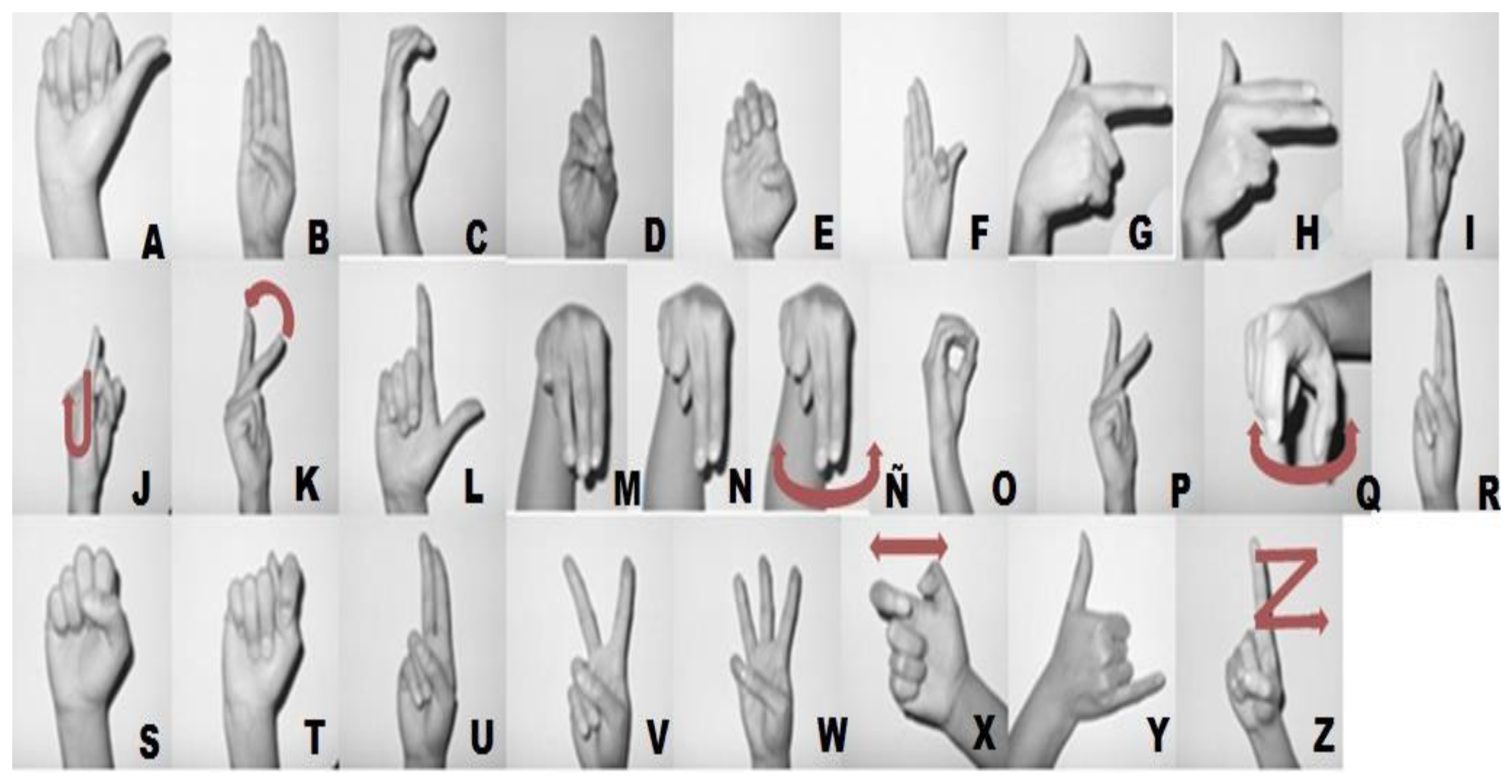
In this work, we concentrate on the MSL alphabet, which has 27 letters. Of these, six letters are dynamic, and 21 are static. Our learning and recognition method focuses on the 21 static letters (A, B, C, D, E, F, G, H, I, L, M, N, O, P, R, S, T, U, V, W, and Y) (Figure 1) [8].
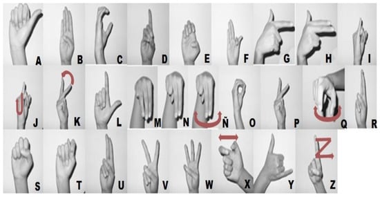
Figure 1.
Sign language alphabet. The six letters drawn with arrows are dynamic. Other authors include three additional dynamic letters: CH, LL, and RR [8]. The remaining 21 letters are the static signs that are recognized in this work.
The main contributions of this research are as follows:
- The proposed method can learn and recognize letters from the MSL static alphabet in indoor conditions using a depth camera. It does not require a special background, and the user does not need to wear special clothes or gloves.
- Our method is invariant to 3D translation, scale, and rotation as far as the same side of the hand is captured from the sensor.
- It provides an interpretable 3D shape feature representation based on three types of geometrical features of the normalized shape. The first type of feature is the proportion of 3D points in each of the spherical sectors, the second type is the average distance to the centroid from the spherical sectors, and the third is the proportion of points inside a Cartesian division of a 3D cube.
- On the test dataset, this classification scheme achieved a precision of 100%, which was higher than other comparable methods for MSL. Our study also included more participants than previous works on the whole static MSL alphabet.
The structure of this work is as follows. Section 2 describes the proposed method, the acquisition environment, and the dataset used. In Section 3, the experiments and results are explained. Section 4 presents a discussion of the results and compares our method with other related works. Finally, Section 5 describes the conclusions and limitations of the study and suggests directions for future work.
Related Works
For several decades, researchers have studied gesture recognition using sensors or vision-based approaches [10,11]. It is estimated that 77% of the research in this area is based on vision [11]. Gesturing may involve the body, hands, head, and facial expressions [10]. Hand gestures may be static or dynamic [10], and dynamic gestures may be isolated or continuous [10].
Of the various body parts involved in gesturing, it is estimated that the use of only one hand corresponds to 21% [11]. The main vision-based representations are model-based and appearance-based [10,11]. Model-based approaches can be further divided into 2D and 3D models [10]. A 2D model representation includes color, silhouette, and a deformable Gabarit model [10,11]. The 3D model-based representations can be further divided into 3D textured volumetric, 3D geometric, 3D skeleton, and 3D skinned mesh models [10,11]. Appearance-based approaches can be divided into shape/color/silhouette-based models, template models, and motion-based (optical flow, motion template) models [10,11]. The representation used in this paper can be considered as a 3D geometric model based on statistics. A structural representation of the hand geometry is based on a 3D model, joint constraints, and a regression scheme to find instances of the hand [12]. For monocular systems if there are finger occlusions the results can present errors [12]. Recently, these types of regressors have improved using deep learning on databases of thousands of images [13]. Since our classification problem only has 21 classes, our method uses a simpler approach, which is less expensive computationally to train and to test.
The main applications of gesture recognition are within the areas of virtual reality, robotics and telepresence, desktop and tablet PC applications, gaming, entertainment, and sign language recognition (17.9%) [11].
The challenges currently faced by vision-based gesture recognition models are related to the system (response time, cost factor), the environment (background, illumination, invariance, ethnic groups), and the gestures (translation, rotation, scaling, segmentation, feature selection, dynamic gestures, size of dataset) [11]. Most gesture recognition systems are based on a general architecture that includes preprocessing (segmentation, tracking), gesture representation (gesture modeling, feature extraction), and recognition (classification) [10].
For vision-based approaches to sign language recognition, the input may be a color image or video, or a depth image or video [11]. Recognition of a hand sign may involve its shape, orientation, location, and movement [11]. A sign that does not require the hands may involve mouth gestures, body posture, or facial expressions [11].
There are several approaches to sign language recognition; one way of classifying these approaches is into those that use hand-crafted features and those that use deep models. The use of the latter type of model requires large-scale, high-quality labeled datasets [14].
Research into the development of automatic methods for the recognition of many sign languages is ongoing all over the world. The language that has been the subject of most studies and has the highest number of available datasets is American Sign Language (ASL). One recent work by Yang et al. concentrated on finger spelling recognition using a depth sensor and a receptive field-aware neural network [15].
Since research into MSL is less well developed than that on ASL, and since public databases of MSL do not exist, we will concentrate in this section on related works on MSL and shape recognition methods that have used spherical representations.
The related works on the recognition of MSL are summarized below. There are some studies that have aimed to recognize dynamic signs, while others have focused on static signs. Some of the features of our work which represent improvements over previous research on MSL are that our system does not require a controlled background, allows for 3D pose changes, and achieves higher accuracy.
First, we describe studies on the recognition of dynamic MSL words (Table 1), and we then summarize the research on static MSL recognition (Table 2). Our work only involves recognition of static alphanumeric MSL gestures (Table 2). It is important to mention that the static MSL alphabet has only 21 letters [8], and we followed this convention in our study. The MSL alphabet also contains dynamic letters such as CH, J, K, LL, Ñ, Q, RR, X, and Z [8]. Some authors have included static frames for some of the dynamic letters as additional classes, but these are not used as part of the static MSL alphabet. We mention this in order to explain why some studies have reported more than 21 static alphabet letters (Table 2). Artificially adding static frames for dynamic letters as additional classes is not valuable to the end user, since the nature of these letters means that they must be recognized dynamically.

Table 1.
Comparison of MSL recognition methods for dynamic signs (words).
Table 2.
Comparison of MSL recognition methods for static alphabet letters or numbers.
Prior works on the recognition of dynamic MSL words are as follows. Cervantes et al. presented a method that could recognize 249 dynamic MSL words in a controlled environment [16]. Videos of 22 persons were created using a black background and black clothes. After processing and segmentation of the hands, 743 geometric, texture and color features were extracted for each segmented region. A genetic algorithm was then used for feature selection, and finally, a support vector machine classifier was used for training and classification of a test dataset. An average accuracy of 97% was obtained.
Sosa-Jimenez et al. developed a real-time MSL recognition system [17] that recognized 33 dynamic words in an indoor setting, without the need for a controlled background or clothes. Ten participants performed each word five times. The reported metrics were a sensitivity of 86% and a specificity of 80%.
Garcia-Bautista et al. presented a system that could recognize 20 dynamic words from Kinect data with a mean accuracy of 98.57%, for a dataset in which each sign was performed once by 35 participants [18].
Espejel-Cabrera et al. developed a method for the recognition of 249 dynamic words of MSL [19]. Eleven people participated in generating a dataset of 2480 videos, each containing a dynamic word. A few representative frames were selected from each video, and a neural network was used to segment the face and hands using color information in the HSV space. Geometric features were extracted from the region of interest, and a support vector machine was used for classification. The average precision was 96.27%, although for nine of the words the accuracy was lower than 70%.
Mejia-Perez et al. assessed different architectures of recurrent neural networks (RNNs) for the recognition of 26 dynamic words and four static alphabet letters [20]. Four people performed each sign 25 times against a controlled background while wearing black clothes. A total of 3000 short videos were collected. The authors used 67 3D key points as features obtained from the face, both hands and the body. The accuracy obtained was 97% on the test set without noise, and 90% with noise.
Research works on the recognition of static MSL alphabet letters or numerical digits are as follows. One of the first was by Luis-Perez et al., who reported a method that could recognize 23 static letters of the MSL alphabet from color images [21]. In this work, a static capture of two dynamic letters (Q, X) was included as part of the 23 symbols. They used active contours for segmentation, and then applied a shape signature for shape description, followed by a neural network classifier. They achieved a recognition rate of 95.8% on their dataset (Table 2). The gestures in the dataset were performed by only one person, clothing was used to ensure that only the hand was visible, and the posture was fixed in 2D. The background also created a strong contrast with the hand. This system only works under controlled conditions and was not tested with other signers. On the application side, they used eight MSL letters to command the movements of a simulated and a physical robot.
Priego-Perez presented two methods in his work [22]. The first used RGB images, and the posture of the hand could vary in 2D through translation, rotation, and some scaling. The illumination and background were controlled to aid in segmentation. Hu moments and other 2D descriptors were then used in a rule-based system to carry out classification. The author reported a classification accuracy of 100% for 20 letters of the MSL alphabet under these experimental conditions and with only two subjects. The static letters H, N, P, and U were excluded from the dataset, and still images of the dynamic letters K, Q, and X were used. However, this method did not permit 3D changes in pose. The second proposed method allowed for more variation in the distance between the subject and the Kinect camera, and depth was used to segment the hand in the image. The author developed a 2D template for each letter using evolutionary matrices, and classification was completed using a distance metric. In this method, 25 letters of MSL were recognized with 90% accuracy, with two signers. Of these 25 letters, 21 were standard static letters and the remaining four were static frames from the four dynamic letters (K, Q, X, and Z).
Trujillo-Romero et al. reported a method for recognizing 27 letters of the MSL alphabet from 3D posture [23]. Of these 27 letters, six were still images of the dynamic letters J, K, Ñ, Q, X, and Z. These authors achieved a precision of 90.27% with one test signer.
Solis-V et al. used 2D normalized geometric moments and a neural network to recognize 24 static signs from MSL, achieving a recognition rate of 95.83% [24]. Of the 24 signs, 3 were still images of the dynamic signs K, Q, and X. One person performed each sign five times using a solid white background. This scheme took RGB images as input.
Galicia et al. used Kinect sensor data (image, depth, skeleton) and geometric distance as features, together with random forest and neural networks, to recognize five vowels and two constants from MSL with a precision of 76.19% [25].
Solis et al. applied Jacobi–Fourier moments to recognize 24 signs from the MSL alphabet using RGB images [26]. Of these 24 signs, 3 were static captures of the dynamic letters K, Q, and X. The moments were 2D rotational invariant. These authors used a dataset acquired from one signer. A neural network was used for classification and achieved a recognition rate of 95%.
Solis et al. used normalized moments and a neural network to recognize 21 signs from the static MSL alphabet using RGB images [27]. The moments were invariant to translation and scale, but not to 2D rotation. The dataset was taken from only one signer, and the recognition rate was 95.83%.
Jimenez et al. recognized five static letters and five numbers [28], using a database that was generated by 100 participants performing each sign once. Their method worked with 3D cloud points and obtained 3D Haar features. The features were classified using an Adaboost classifier, which yielded an F1 score of 95%.
Salas-Medina et al. used a pretrained Inception v3 deep learning network which was then retrained on images representing the MSL static alphabet [29]. The database used for retraining was generated by 10 signers performing each of the 21 static letters 10 times. Each image was manually cropped to select the hand region. This system achieved an accuracy of 91%.
Carmona-Arroyo et al. recognized 21 static MSL letters using six 3D affine moment invariants [30]. The dataset was generated by nine signers, who performed each sign once. The input was a 3D point cloud for each sign. The precision was 95.6% when a MS Kinect 1 sensor was used, and 94% on a different dataset generated with a leap motion sensor.
In summary, the main improvements offered by the proposed method over other methods of recognizing MSL static alphabet letters are as follows (Table 2): our approach does not require a controlled background; it allows for changes in translation, scale, and 3D pose; we use 15 signers (i.e., more than other methods) for the whole static alphabet; and our model is superior to other methods in terms of accuracy.
Other works related to the proposed method involve the use of spherical representations for computer graphics, computer vision, and pattern recognition. Some representative examples of these works are described below.
Takei et al. presented a method for fast 3D feature description. They estimated key points and descriptors by counting the occupancy in spherical shell regions. These descriptors were invariant to 3D rotation and allowed for object recognition [31].
Roman-Rangel et al. presented a method for describing points of interest in a 3D point cloud [32]. Their method computed two histograms: one for the local distribution of orientations in terms of azimuth angles, and one for the zenith angles. The orientations between a reference point and points within a spherical neighborhood were computed.
Hamsici et al. provided a general method for shape analysis based on kernels that were invariant to 3D translation, scale, and rotation [33].
Garcia-Martinez et al. proposed a scale- and rotation-invariant 3D object detection scheme using correlations on the unit sphere [34].
Ikeuchi et al. presented a method based on spherical representations for recognizing 3D objects [35]. It was shown that extended Gaussian, distributed extended Gaussian, complex extended Gaussian, and spherical attribute image representations were best suited to certain surface geometries depending on the task.
Previous works have used spherical representations, but in some cases, these are general methods for shape recognition or for specific applications [31,32,33,34,35]. They have not been applied to sign language recognition, and the details of these methods are different from the proposed approach.
2. Materials and Methodology
A Kinect 1 sensor was used for the acquisition of the 3D point cloud for each static letter. The sensor was placed on a tripod at a height of 1.3 m, and the participants were located 1.5 m from the sensor. Indoor illumination was used with no special background.
The software used was Matlab 2015, which was run on a Dell G5 15 laptop with the following specifications: 16 GB RAM, six 8th generation Intel i7 cores, 2.21 GHz (12 logical processors), 100 GB SSD, 1TB HD, Windows 10 Home, Nvidia Geoforce GTX 1050 Ti (4 GB GPU memory), Intel UHD Graphics 630 (8 GB GPU memory).
2.1. Dataset and Participants
Each sign was performed once by 15 participants, who were aged between 6 and 34 and included seven females and eight males. The participants performed each sign after rehearsing it once, as they were not native MSL users. They were told to perform the sign showing the standard pose for each sign being free otherwise, and all participants performed the signs with their right hand. For the 21 signs analyzed in this study, a total of 315 point clouds were acquired.
2.2. Preprocessing
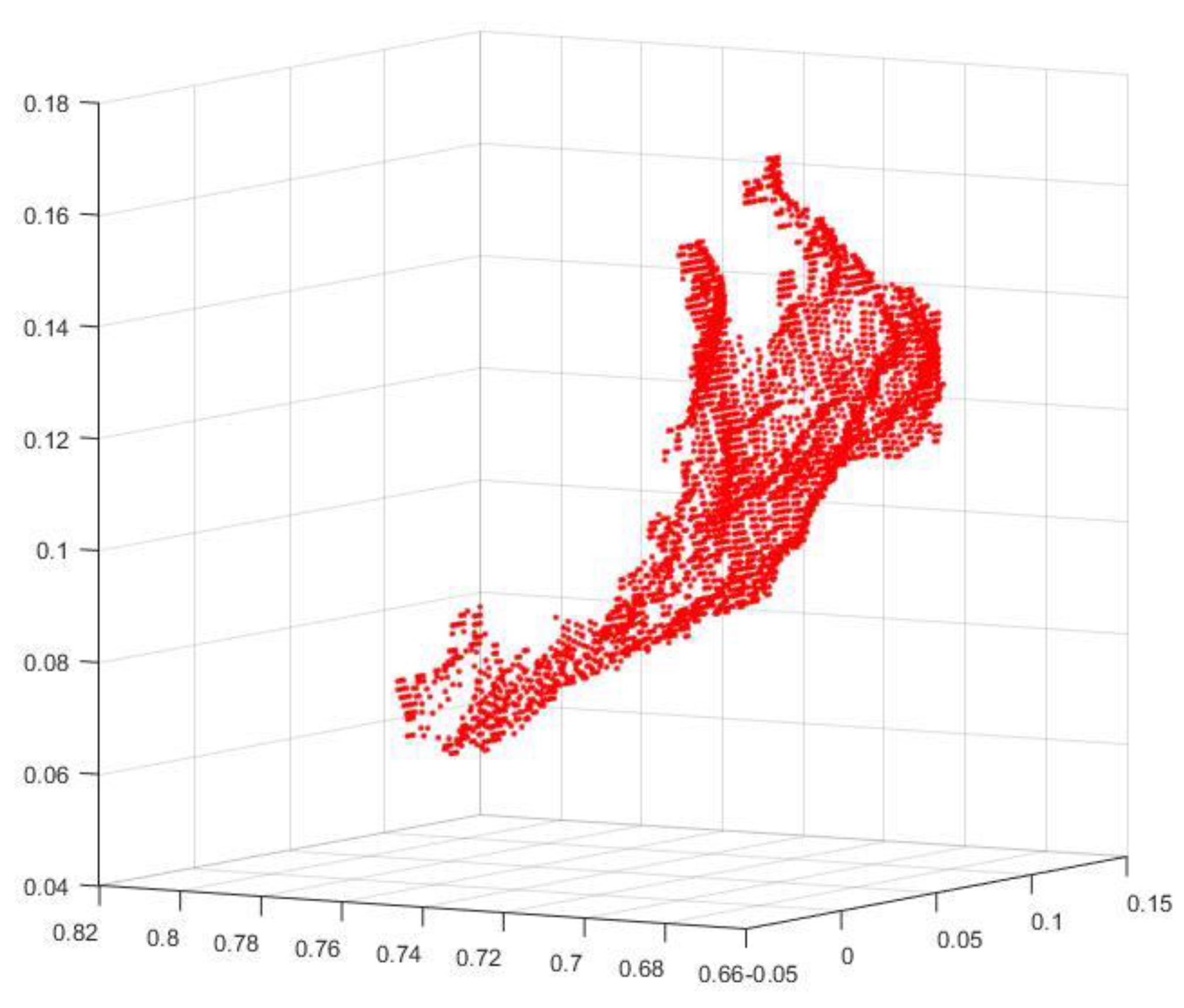
A depth threshold was used to segment the performing arm from the rest of the point cloud, as shown in the example in Figure 2. To further segment the hand from the forearm, a segmentation procedure was implemented that followed the work of Tao et al. [36] and applied palm region approximation, arm region segmentation, and arm region removal to isolate the hand.

Figure 2.
A raw 3D point cloud for Mexican sign language for the letter A. The total number of points is 4061. The X coordinate varies in the range [−0.0217, 0.1074], Y in the range [0.0556, 0.1685], and Z in the range [0.67, 0.8]. Notice that the forearm is present.
2.3. Method
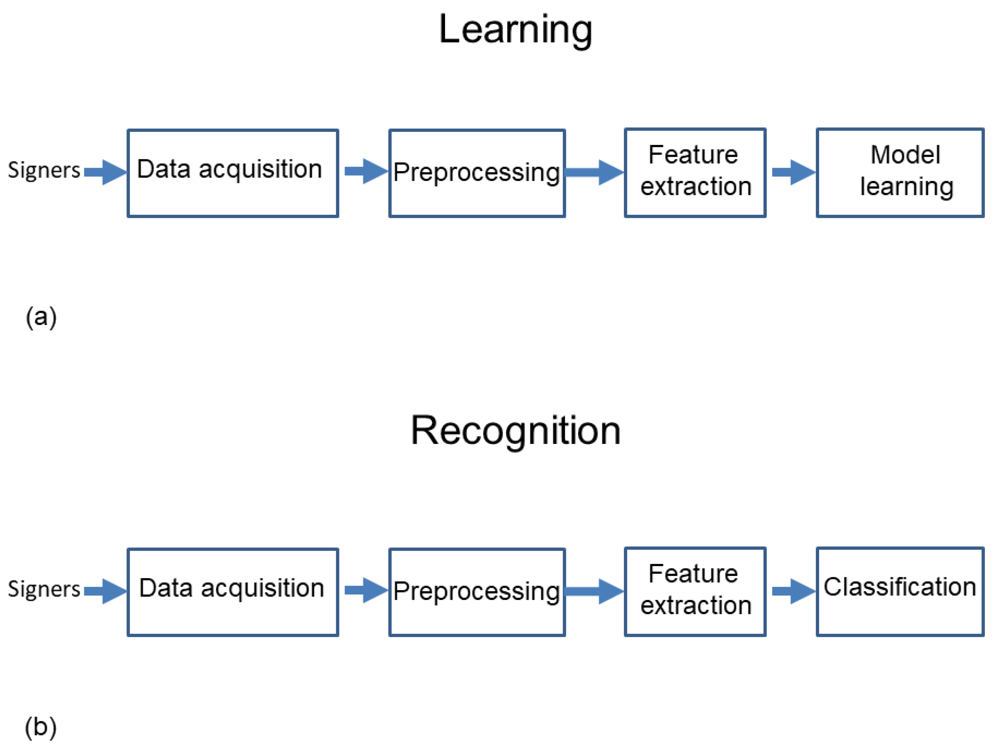
A block diagram of the learning and recognition process is shown in Figure 3.
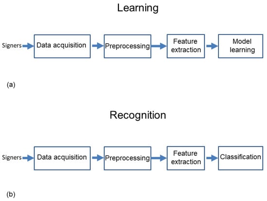
Figure 3.
Main steps in the learning (a) and recognition process (b) of static letters from the Mexican Sign Language alphabet, using features derived from the partition of a unit sphere and a cube containing a normalized 3D point cloud.
To achieve invariance to 3D translation, the centroid (Xc, Yc, Zc) was computed for each file, as shown in Equations (1)–(3):
where N is the total number of points in the file and is different for each. (Xi, Yi, Zi) correspond to generic points in each file.
Then, new updated coordinates invariant to 3D translation are computed by subtracting the centroid as shown in Equations (4)–(6):
To achieve invariance to 3D scale, the coordinates of each file are updated to fit inside a sphere of radius one as follows:
where are the new updated coordinates that are invariant to scale, and MaxNorm is the maximum norm of each 3D point cloud.
To achieve invariance to 3D rotation, a new coordinate system is computed by applying a principal component analysis (PCA) to each data file and following the procedure below.
The first eigenvector e1, which explains most of the variance in the data, becomes the vertical axis Y. The second eigenvector e2, which explains the variance in the data in second place, becomes the horizontal axis X. Finally, the third eigenvector e3, which explains the variance in the data in third place, becomes the depth axis Z.
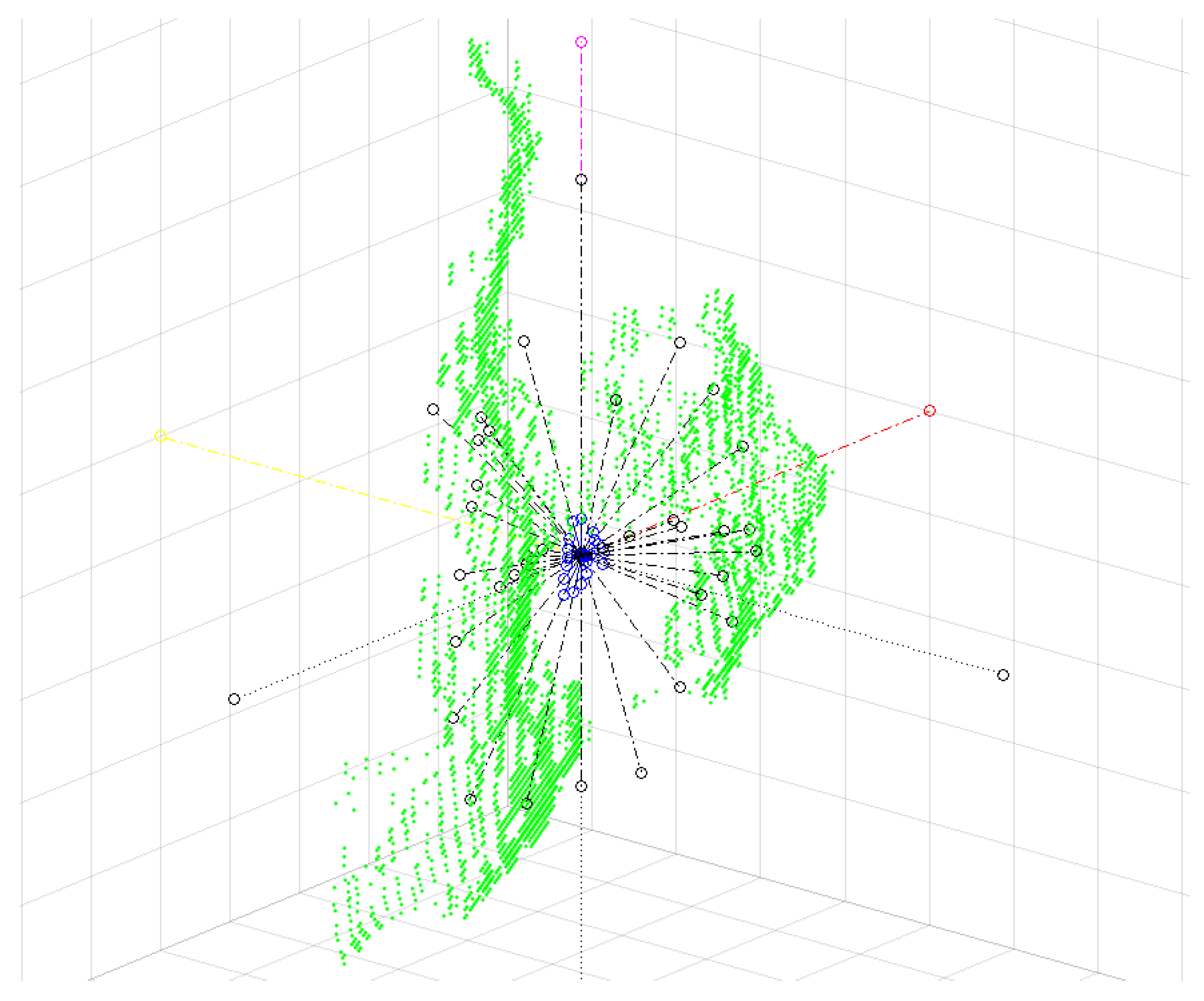
The data are then transformed to the new (e1, e2, e3) coordinate system as shown in Figure 4. Since the transformed data are now inside a unit sphere, we define three types of features, two of which are derived using a spherical coordinate system, and the third is obtained using a Cartesian coordinate system.
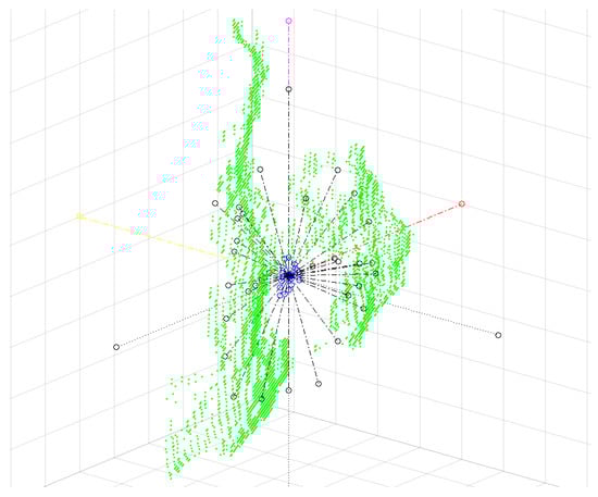
Figure 4.
An MSL sign for the letter A, normalized in translation, scale, and rotation, showing the principal axes. The positive Y axis is shown in magenta, the positive X axis in red, and the positive Z axis in yellow. The average distance features in each spherical sector are shown in black, and the probability for each spherical sector is shown in blue.
Using the new axes, a spherical coordinate system (θ,φ) is defined. Let θ be the azimuthal angle in the X-Y plane, where , and let φ be the polar angle, where measured from the Z axis. The intervals of the azimuthal and polar angles are divided uniformly. Let binsθ be the number of subintervals (bins) into which the range [0,2) of angle θ is divided, and let binsφ be the number of subintervals into which the range [0,) of angle φ is divided. For our experiments, we tried several combinations. The values that gave us the best results were binsθ = 18 and binsφ = 3.
The first type of feature is the probability of finding 3D points in each spherical sector (Figure 4). We use a spherical histogram H(θi, φj) to count the number of 3D points that fall inside the sector (θi, φj), where i = 1…binsθ, j = 1…binsφ.
A discrete probability distribution P(θi, φj) can be defined for each file by normalizing by the total number of 3D points N in the file, as shown in Equation (11):
Converting this to a discrete probability distribution allows us to compare the similarities and differences between signs; this probability is also independent of the number of points in each file, which can vary. For the first type of feature, we have a total of 18 × 3 = 54 features, one for each spherical sector.
The second type of feature is the average distance in each spherical sector from the origin (Figure 4). Here, () are the spherical coordinates inside a spherical sector, and means the average distance of all the points in the 3D cloud from the origin in a particular spherical sector. Again, we have a total of 18 × 3 = 54 features.
In summary, for each spherical sector, we take as features: (i) the probability and (ii) the average distance from the origin In total, 54 + 54 = 108 features are obtained from the spherical sectors.
For the third type of feature, a Cartesian coordinate system is defined using the new axes. To derive the features, the intervals [−1,1] on the X, Y, and Z coordinate axes are uniformly divided into subintervals. The numbers of subintervals on each axis that gave us the best results were binsY = 17, binsX = 3, binsZ = 2, where binsX, binsY, binsZ are the numbers of subintervals on the X, Y, and Z axes, respectively.
The third type of feature is the probability in each Cartesian subinterval (Figure 5). Here, Hc(Xi, Yj, Zk) is the histogram that counts the number of points in the subinterval (Xi, Yj, Zk), where i = 1…binsX, j = 1…binsY, k = 1…binsZ. The probability PC in each Cartesian subinterval is given by Equation (12):
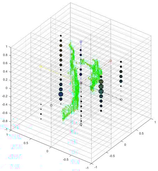
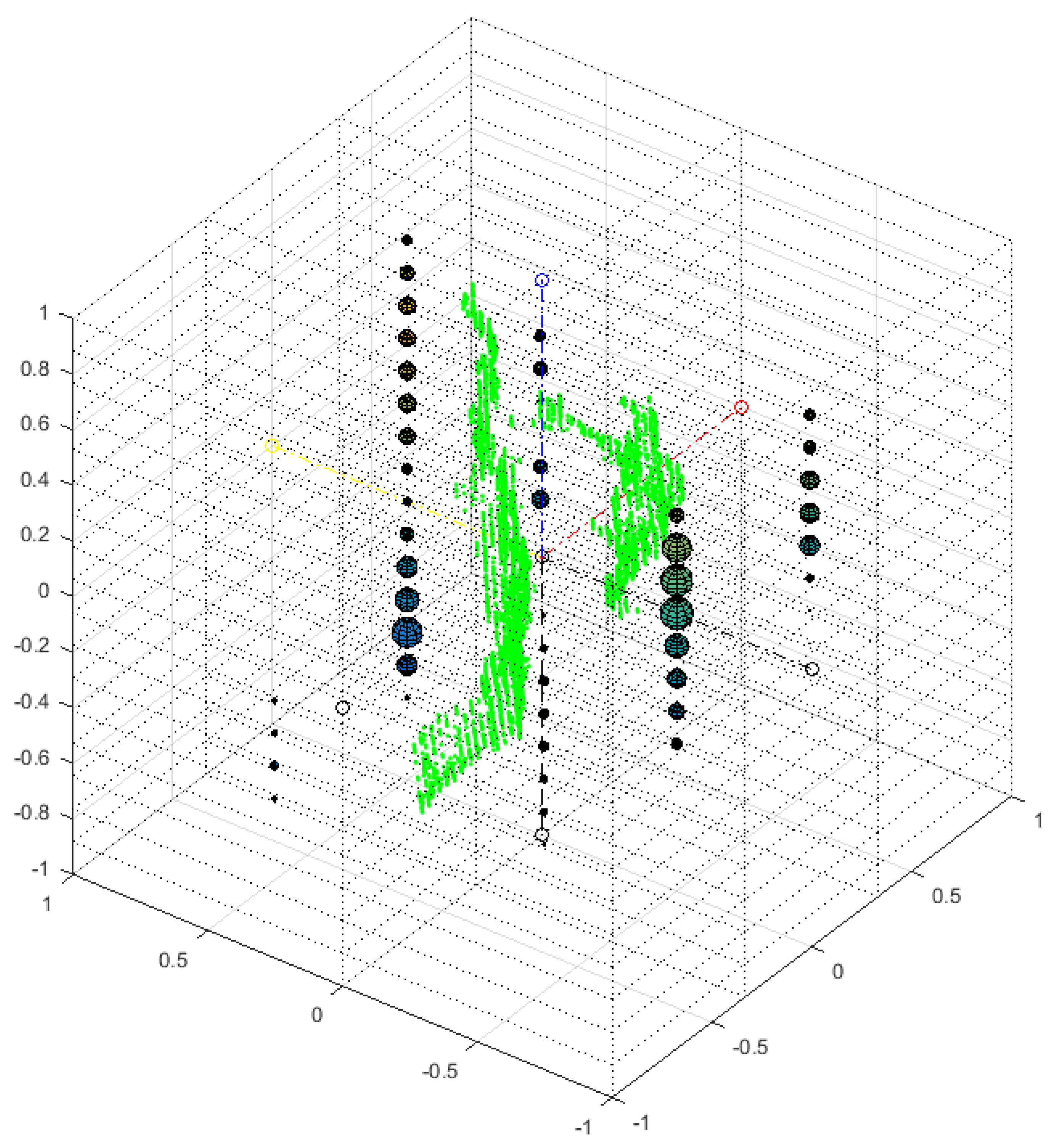
Figure 5.
An MSL sign for the letter A, showing the Cartesian features in a 3D rectangular grid. The size of each sphere is proportional to the number of 3D cloud points in each sub-rectangular prism.
The Cartesian subintervals are used to complement the spherical subintervals, since they generate a different partitioning of the data and hence different features. Since the vertical Y axis obtained through PCA explains most of the variance in the data, it has a higher number of divisions, BinsY = 17. The horizontal X axis defined by PCA, which explains the remaining variance in the data in second place, is divided into BinX = 3. Finally for the Z axis, which provides depth along the third axis defined by PCA, the subintervals are BinsZ = 2. This third type gives 2 × 3 × 17 = 102 features.
To represent each sign, the features from the spherical sectors and the Cartesian rectangular prisms are then concatenated, giving 54 + 54 + 102 = 210 features.
To represent each class of signs, a Gaussian distribution is obtained by maximum likelihood estimation (MLE) from the features of the normalized examples as shown in Equation (13):
where is the Gaussian of the kth class (k = 1…21), is its mean, and is its covariance matrix. represents sample m (or example m) for class k, where m = 1…MaxSam, and MaxSam is the maximum number of examples.
If we assume that all sign classes are equally likely, for a new sample sign s*, it is possible to predict the most likely class by a maximum a posteriori (MAP) approach, as shown in Equation (14):
where represents sign class α, and represents the probability that the sample sign s* belongs to class k. In other words, the predicted class is the one with the highest probability. All the existing sign classes are tested.
3. Experiments and Results
To assess our method on a dataset, a cross-validation procedure with k = 15 was used. A leave one person out (LOPO) strategy was applied, meaning that for a particular fold, all 21 letters signed by one person were used for testing, and the training was completed on the letters (14 × 21 = 294) from the remaining 14 signers. This means that for each fold, 14 examples were used for training each letter class, and a different letter from each class was used for testing. The accumulated confusion matrix resulting from the cross-validation procedure was used to derive the values of the performance metrics, as shown in Equations (15)–(19) below.
A diagonal covariance matrix was used to train the multivariate Gaussian representing each class in each fold, as shown in Equation (13).
The supervised learning procedure from Matlab that was used in each fold to train and predict a class for the test elements using MAP (14) was ‘classify’, with parameter ‘diaglinear’.
Three experiments were carried out, as follows:
- Training and classification using only spherical features (108 features).
- Training and classification using only Cartesian features (102 features).
- Training and classification using spherical and Cartesian features (108 + 102 = 210 features).
To analyze the classification performance of the model in each experiment, six metrics were used as defined in Equations (15)–(19), with the area under the curve (AUC) for the received operating characteristics (ROC) curve [37].
where TP, TN, FP, and FN refer to true positive, true negative, false positive, and false negative results, respectively.
The results of the experiments are as follows. For Experiment 1, the accumulated confusion matrix using only spherical features is shown in Figure 6. The values of TP, TN, FP, and FN, and the metrics for each class corresponding to the confusion matrix in Figure 6 can be seen in Table 3.
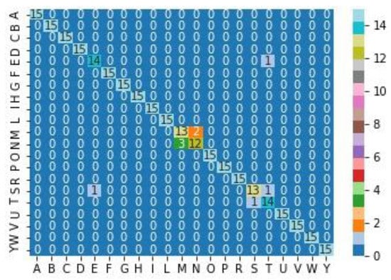
Figure 6.
Cumulative confusion matrix for spherical features from cross validation with k = 15. Rows show the actual classes, and columns show the predicted classes. The confusion matrix (i,j) displays the total numbers of test examples with the actual class i and predicted class j.
Table 3.
Numbers of false negatives (FN), false positives (FP), true negatives (TN), and true positives for each class from the confusion matrix for spherical features in Figure 6. For each class, the metrics of accuracy (Acc.), precision (Pre.), recall (Rec.), specificity (Spe.), F1 score, and area under the curve (AUC) of the received operating characteristic (ROC) are computed. The last row E(.) displays the average for each column.
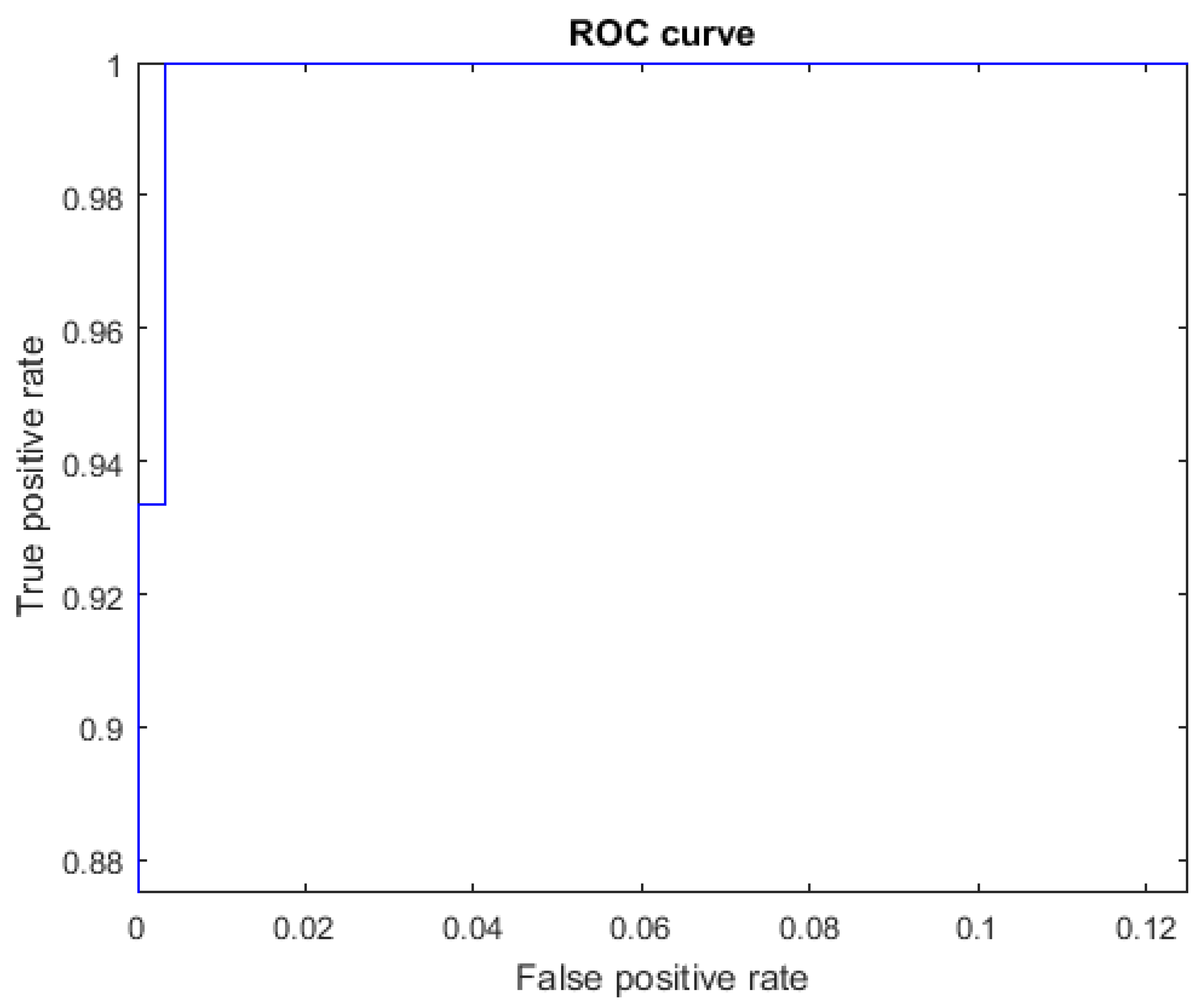
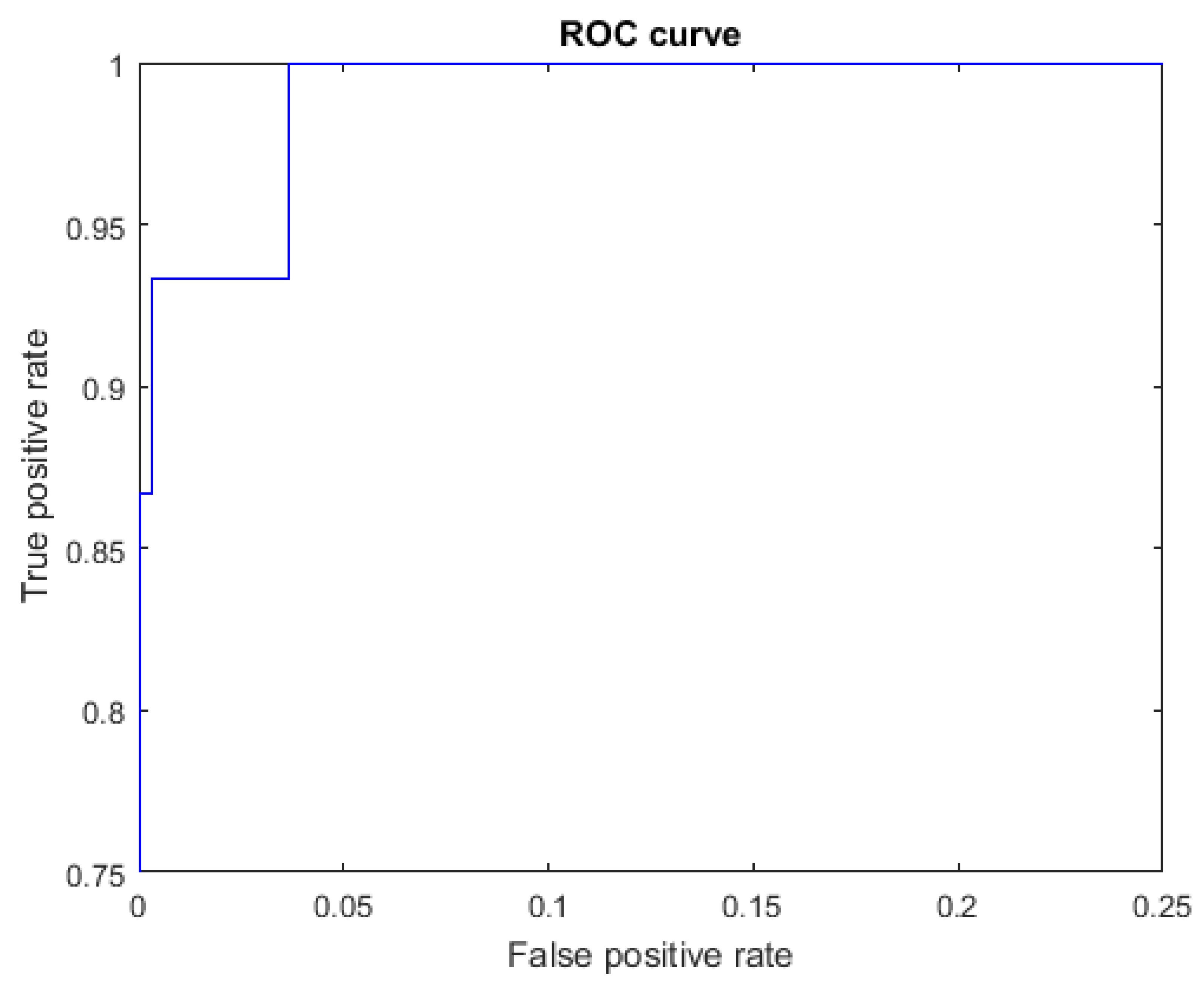
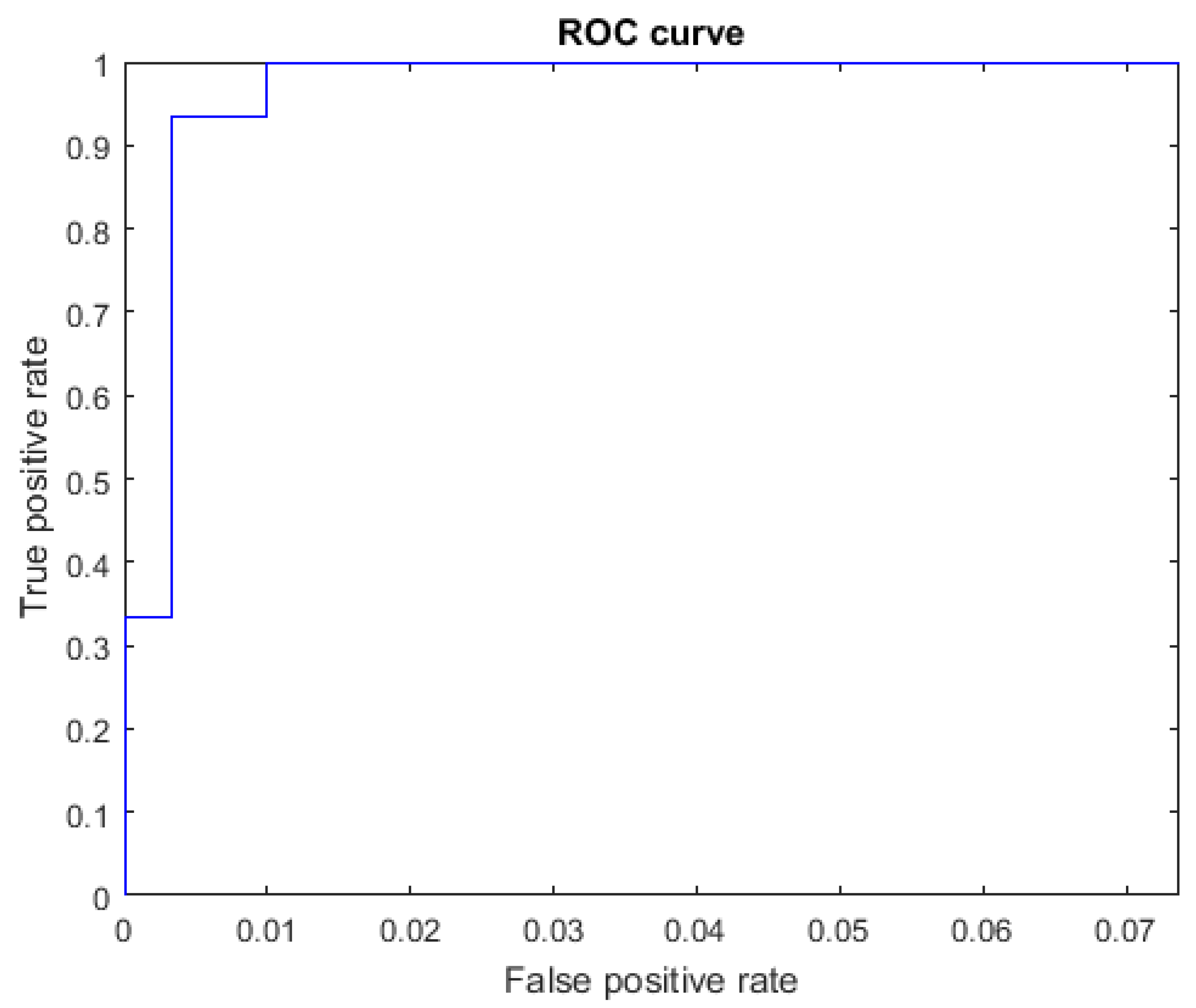
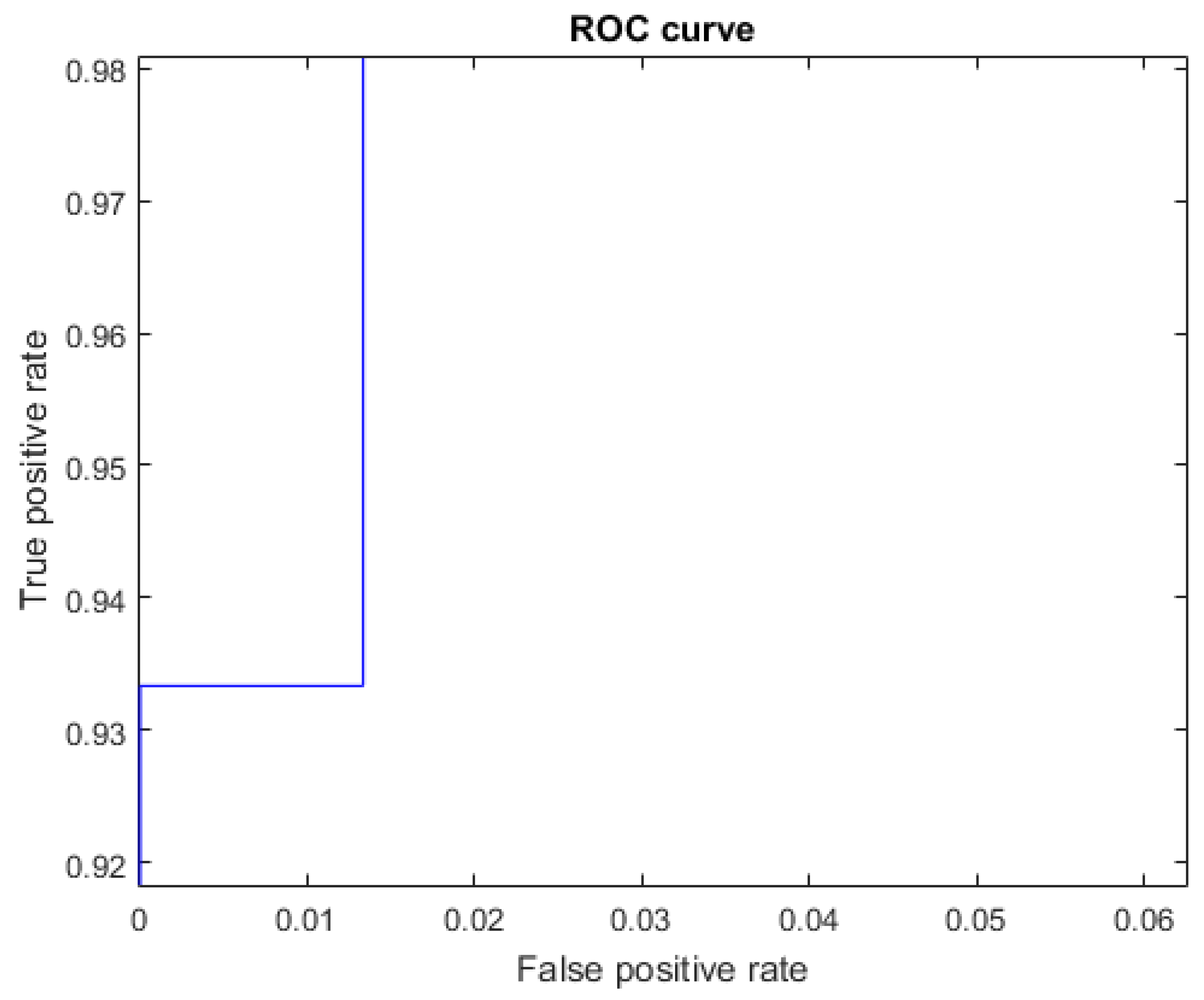
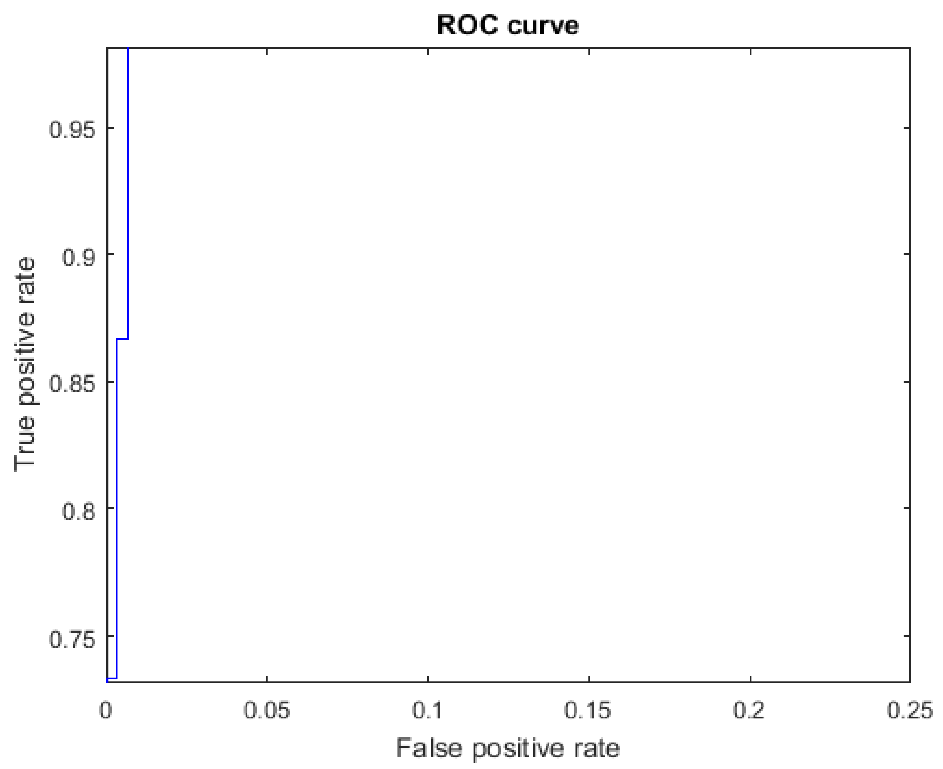
The ROC curves for letters where the AUC was not equal to one are shown in Figure 7 for the letter E, Figure 8 for the letter M, Figure 9 for the letter N, Figure 10 for the letter S, and Figure 11 for the letter T. The other ROC curves were not drawn, since for these, AUC = 1.
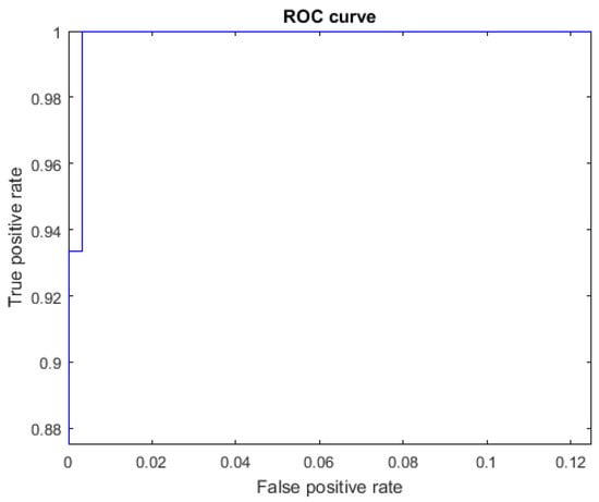
Figure 7.
ROC curve for the letter E using spherical features, AUC = 0.9998.
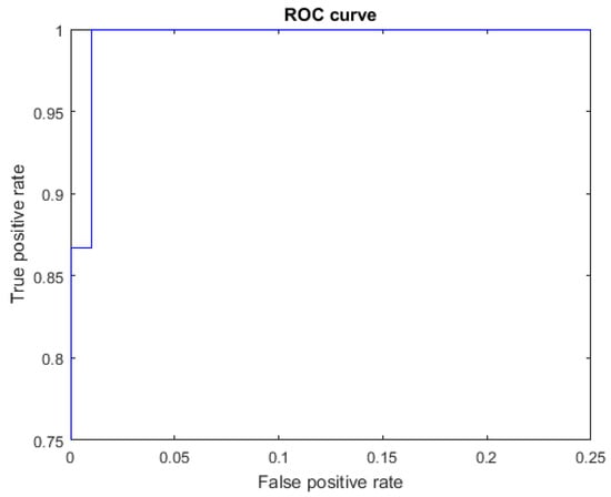
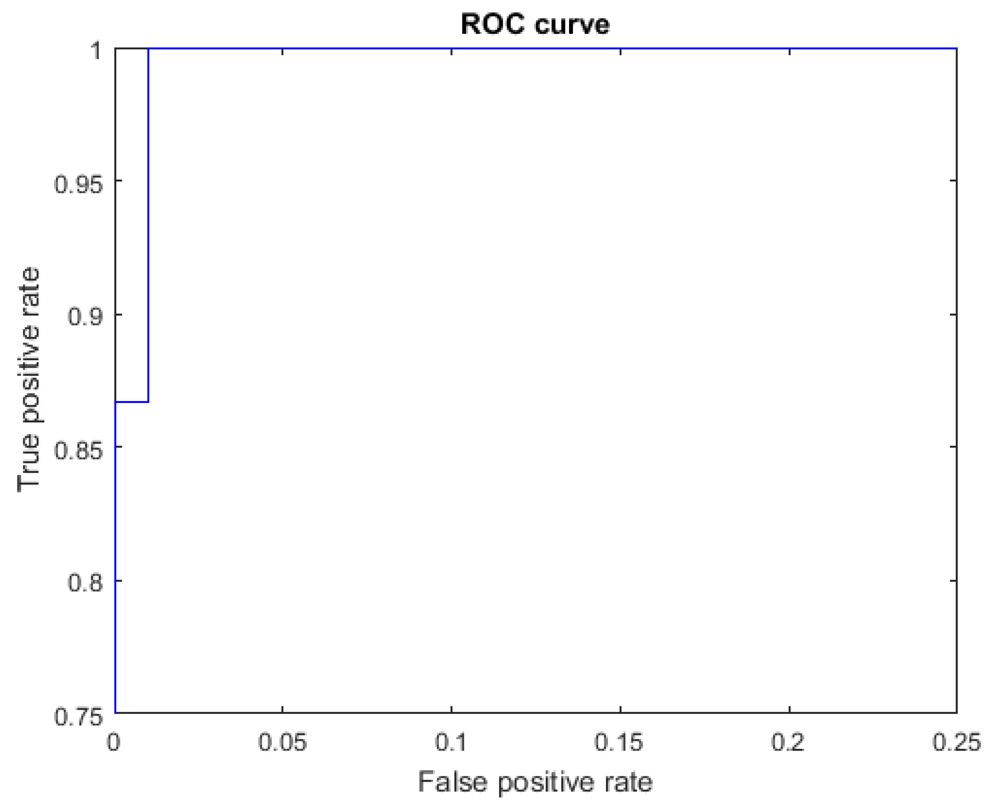
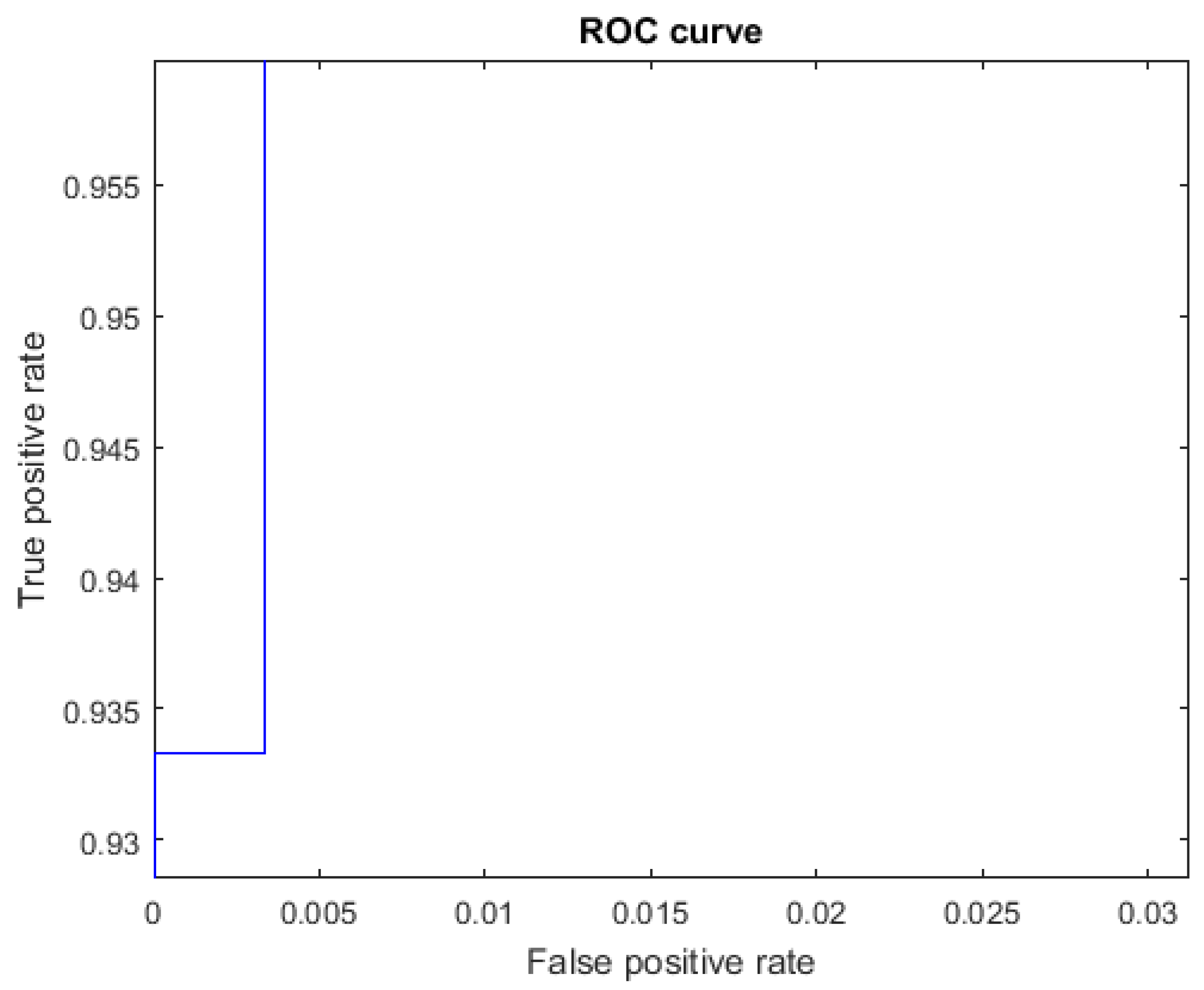
Figure 8.
ROC curve for the letter M using spherical features, AUC = 0.9987.
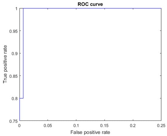
Figure 9.
ROC curve for the letter N using spherical features, AUC = 0.9987.
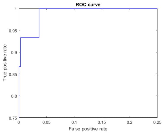
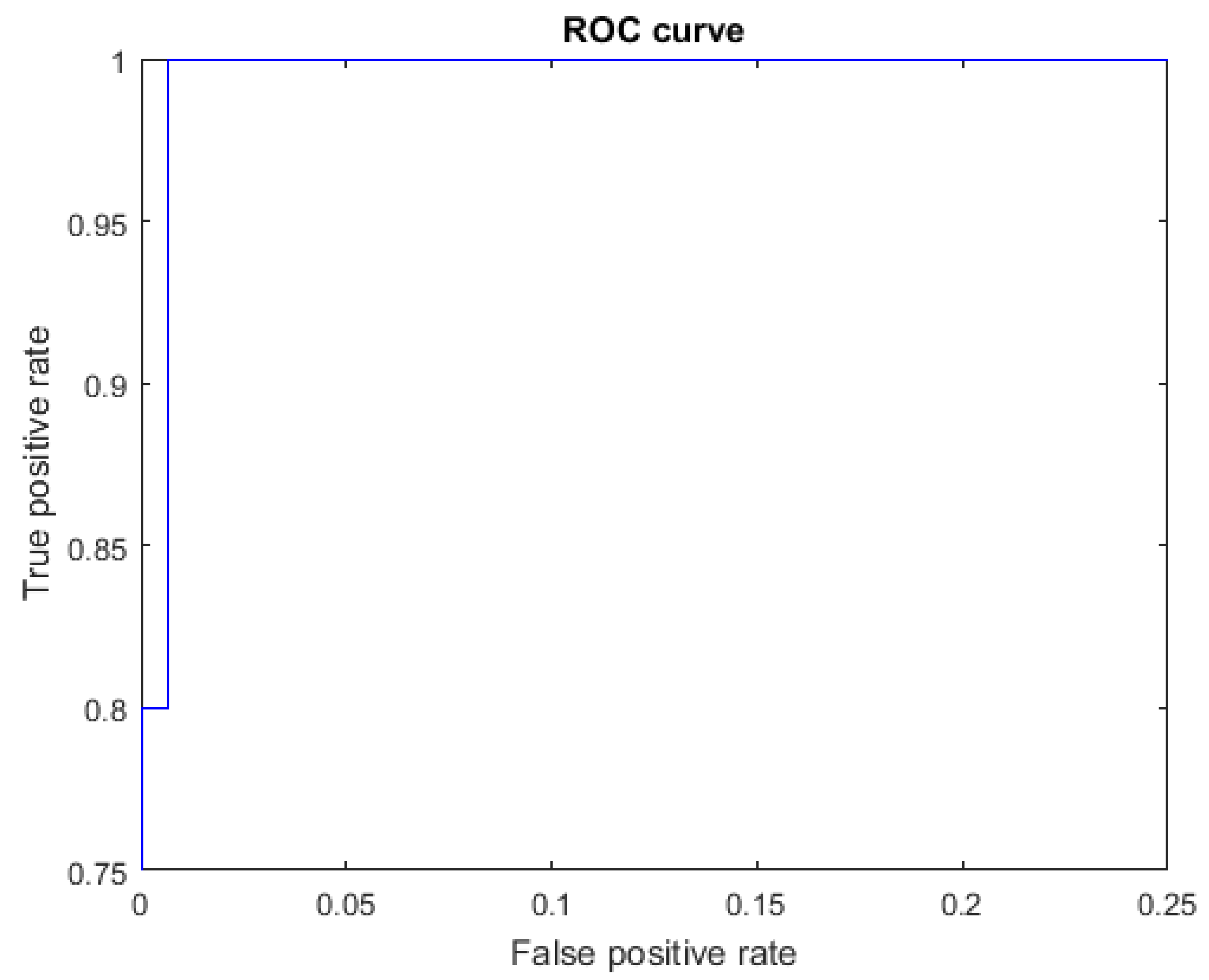
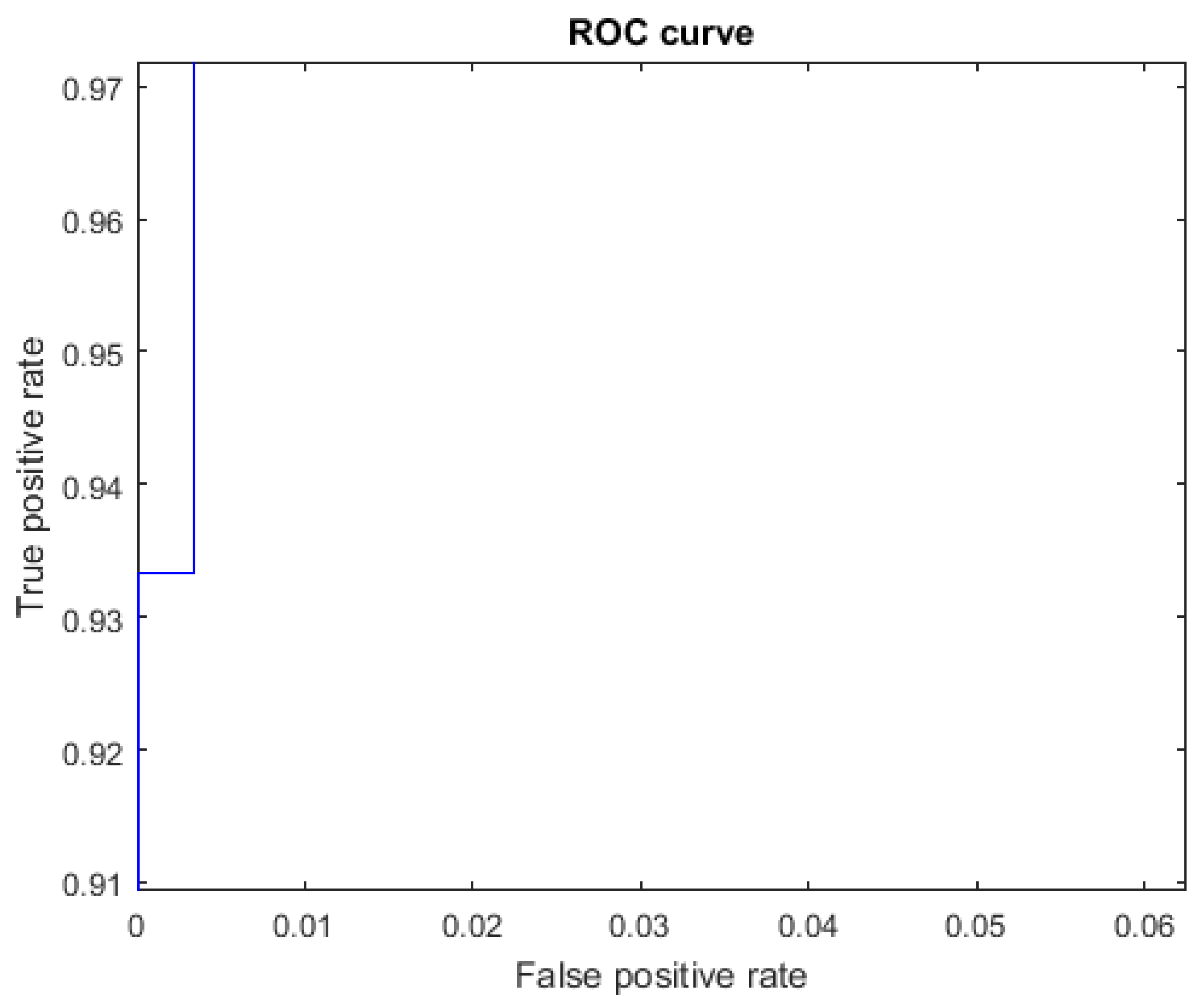
Figure 10.
ROC curve for the letter S using spherical features, AUC = 0.9973.
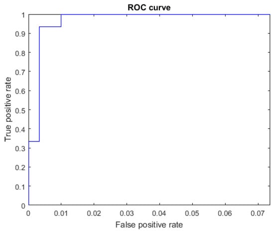
Figure 11.
ROC curve for the letter T using spherical features, AUC = 0.9973.
It is important to mention that in order to generate each ROC curve and the corresponding AUC, it is necessary to provide an identifier for the corresponding class, a label for the class of each example in the dataset, and the prediction score for each example. In our case, the prediction score was generated based on the MAP. Hence, we note that the ROC curves are not obtained directly from the confusion matrix using only TP, FN, FP, and TN [37].
In Matlab, ROC curves were generated using a procedure called “perfcurve” that computes pairs of (false positive rate, true positive rate) varying a threshold and using the abovementioned information.
The values of FN for each letter and signer, corresponding to the confusion matrix of spherical features (Figure 6), can be seen in Table 4.
Table 4.
Numbers of false negatives (FN) by letter and by person, for the confusion matrix of spherical features in Figure 6. Rows show the test letters, and columns show the test signers. For instance, Table(E,12) = T means that for the letter E and signer 12, a false negative was produced (where E was confused with T). The last column ∑ shows the total number of false negatives by letter, and the last row ∑ shows the total number of false negatives generated by each signer.
For Experiment 2, the accumulated confusion matrix using only Cartesian features is shown in Figure 12.
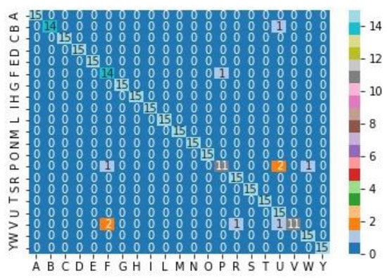
Figure 12.
Cumulative confusion matrix for Cartesian features for cross-validation with k = 15. Rows show the actual classes, and columns show the predicted classes. The confusion matrix (i,j) displays the total numbers of test examples with actual class i and predicted class j.
The values of TP, TN, FP, FN, and the metrics for each class corresponding to the confusion matrix in Figure 12 are shown in Table 5.
Table 5.
Numbers of false negatives (FN), false positives (FP), true negatives (TN), and true positives from the confusion matrix for the Cartesian features in Figure 12, for each class. For each class, the metrics of accuracy (Acc.), precision (Pre.), recall (Rec.), specificity (Spe.), F1 score, and area under the curve (AUC) of the received operating characteristic (ROC) are computed. The last row E(.) displays the average for each column.
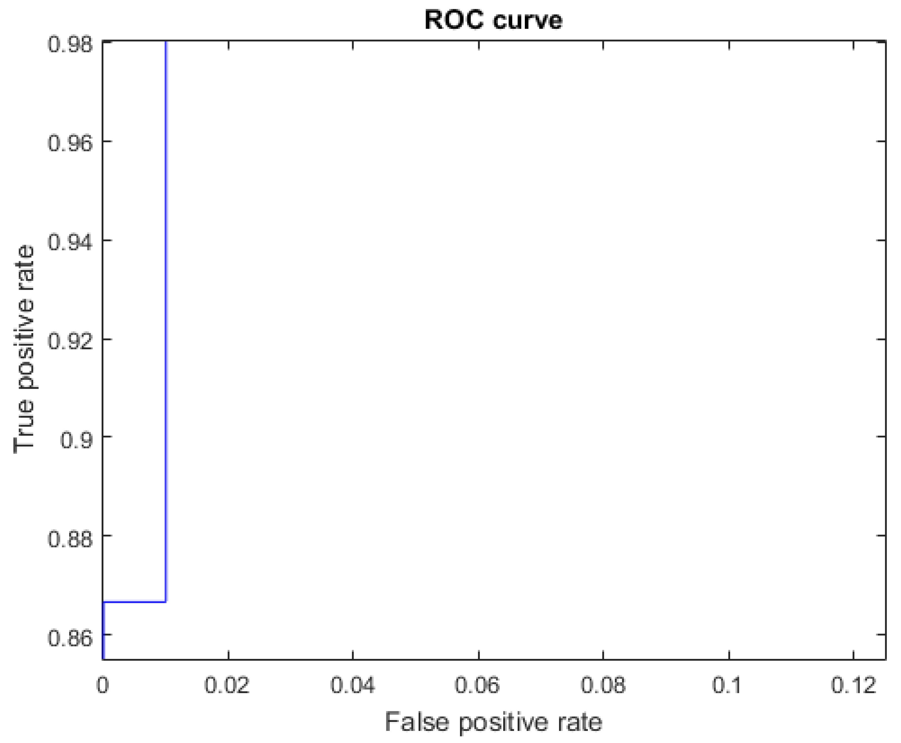
The ROC curves for letters where the AUC was not equal to one can be seen in Figure 13 for the letter B, Figure 14 for the letter F, Figure 15 for the letter P, Figure 16 for the letter R, and Figure 17 for the letter V. The other ROC curves were not drawn, since for these, AUC = 1.
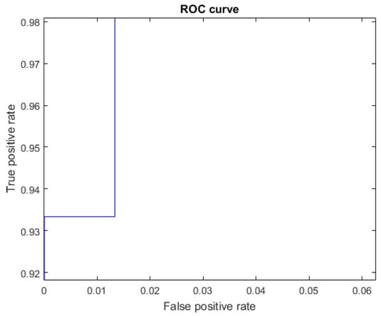
Figure 13.
ROC curve for the letter B using Cartesian features, AUC = 0.9991.
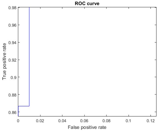
Figure 14.
ROC curve for the letter F using Cartesian features, AUC = 0.9987.
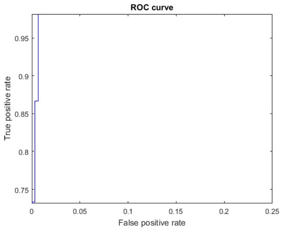
Figure 15.
ROC curve for the letter P using Cartesian features, AUC = 0.9987.
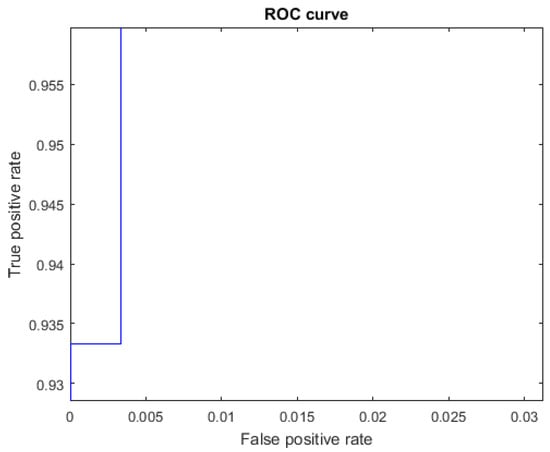
Figure 16.
ROC curve for the letter R using Cartesian features, AUC = 0.9998.
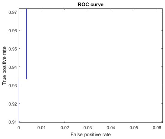
Figure 17.
ROC curve for the letter V using Cartesian features, AUC = 0.9998.
The number of FNs for each letter and person, corresponding to the confusion matrix of Cartesian features (Figure 12), can be seen in Table 6.
Table 6.
Number of false negatives (FN) by letter and by person, for the confusion matrix of the Cartesian features in Figure 12. Rows show the test letters, and columns show the test signers. For instance, Table(B,11) = U means that for letter B and signer 11, a false negative was generated (where B was confused with U). The last column ∑ shows the total number of false negatives by letter, and the last row ∑ shows the total number of false negatives generated by each person.
In Experiment 3, using the spherical and Cartesian features (that is, a total of 210 features), all the elements in the test set were correctly classified for all folds. As a summary, we show the values of all metrics for all three experiments in Table 7.
Table 7.
Average values of the metrics obtained from three experiments using different combinations of features.
4. Discussion
Each division of the two coordinate systems, spherical and Cartesian, into intervals generates a different grid in sectors that collects statistical information on the normalized geometric shapes. It is more difficult to classify some shapes in one coordinate system than the other.
For example, from an analysis of the classification using spherical features and from Figure 6, Table 3 and Table 4, we see that the letter E had TP = 14, FN = 1, and FP = 1. In one case, it was confused with the letter T, and when classifying letter S, one instance was classified as E. These three letters E, T, and S have certain similarities in that each of them involves bending the four fingers (little, ring, middle, and index) and the thumb in different configurations (Figure 1).
For the spherical features, we see from Figure 6, Table 3 and Table 4, that for the letter M, we have TP = 15, FN = 2, and FP = 3, and for the letter N, we have TP = 12, FN = 3, and FP = 2. Two instances of M were misclassified as N, and three instances of N were misclassified as M. This is not surprising, since these two letters are very similar and differ only in the position of the ring finger (Figure 1). This meant that the lowest metrics were achieved for these letters. The precision for the letter M was 0.8125 (i.e., the fraction of predictions as a positive class that were positive) and the recall was 0.8677 (i.e., the fraction of all positive samples correctly predicted as positive). For the letter N, we obtained 0.8571 for the precision and 0.8 for the recall.
For the spherical features, we see from Figure 6, Table 3 and Table 4, that the results for the letter S were TP = 13, FN = 2, and FP = 1. One instance of S was misclassified as T, and another instance was misclassified as E. For the letter T, we have TP = 14, FN = 1, and FP = 2. One instance of T was misclassified as S. The letters S and T are very similar, as they involve a closed fist and only differ in the position of the thumb (Figure 1).
For the spherical features, Table 4 shows the false negatives for each letter and signer. Signer number 12 had more false negatives (2) than the other signers.
For the Cartesian features, we see from Figure 12, Table 5 and Table 6, that the results for the letter B were TP = 14, FN = 1, and FP = 0. One instance of B was misclassified as U. These two letters have some similarity, in that they both involve an extended palm with the index and middle fingers in an upright position. The thumb is also bent similarly. The difference is that for the letter U, the little and ring fingers are bent (Figure 1).
We also see from Figure 12, Table 5 and Table 6, that for the Cartesian features, the letters P and V had the worst recall value of 0.7333, since for both letters the results were TP = 11 and FN = 4. Four instances of P were confused with one instance of F, two of U, and one of W. Four instances of V were confused with two instances of F, one of R, and one of U. Here, the similarities were due to parts of the configuration being the same in the normalized position. For example, the configuration of the thumb, little and ring fingers is the same for letters V, R, and U, and they differ only in the positions of the index and middle fingers (Figure 1).
For the Cartesian features, we see from Table 6 that the signers with the most false negatives for the letters that they performed were 11, 7, and 1.
Compared with the other works on MSL static alphabet recognition in Table 2, we can see that our work involved the most subjects in the dataset for the 21 static letters, allows for 3D changes, has no restrictions on the use of an indoor environment, and achieved the highest precision.
Most of the other MSL recognition methods which use RGB images as input rely on controlled background, clothes, and illumination to facilitate the hand region segmentation using histogram thresholding or snakes [21,22,24,25,26,27] (Table 2). Once they do the segmentation, they obtain a 2D binary region whose shape represents a hand, and all the 3D shape information is lost. In contrast, our method preserves the rich 3D shape information of the hand. Salas-Medina et al. do not segment the hand region, but manually crop a subimage around the hand [29]. Then they use a deep learning network to extract features and classify. In this last case, our research used more users and achieved higher accuracy (Table 2).
Compared to the methods that use 3D input for MSL recognition, Priego-Perez, method 2, manually adjusts a depth range to segment the hand in 3D in each case [22]. Then, he projects to 2D to extract features, and the 3D shape information is lost. His method had problems of differentiating between letters G and H.
Trujillo-Romero et al. use RGB and 3D points clouds as input [23] (Table 2). They require controlled conditions since the hand must be at a distance of 1 m ± 5 cm to be properly segmented. Then, they require the hand to be open in a start position to detect fingertips, and then assign a 3D skeleton. Then, all the fingers must be tracked to the final position using particle filtering. Their method presents problem in tracking and assigning the 3D skeleton when there is similarity in the letters, like letters S and O. Our method does not require all these controlled conditions to segment the hand and to recognize the 3D shape.
The method of Carmona-Arroyo et al. uses 3D points clouds as input [30] (Table 2). Their method which used 3D affine invariants is interesting to describe the 3D shape. Our method improves over them in accuracy, possible because we used more features, and because the 3D hands that we used were better segmented.
5. Conclusions
A novel method for the learning and recognition of the MSL static alphabet was presented. This method is invariant to 3D translation and scale and allows for 3D rotation if the view presented to the depth sensor is on the same side of the hand. The method is based on first normalizing each shape in translation, scale, and rotation. The last of these steps is completed using PCA. We then use the intrinsic axis of the normalized shape to define spherical and Cartesian coordinate systems and extract three types of features. The first and second types of features are extracted using a spherical coordinate system and a partition into spherical intervals. The first type of feature is the probability of finding the 3D points in each interval, while the second is the average distance of the 3D points in the interval from the centroid of the shape, and the third is the probability of finding 3D points in each interval in the Cartesian partition.
The shape of each letter class is summarized using a multivariate Gaussian trained on the defined features. Classification of the test letters is completed using an MAP approach over all the classes.
Our model takes as input a depth image of the performing hand in an indoor environment, with no special background or special clothing. It outperforms previous works on MSL static alphabet recognition in terms of the accuracy and the generality of the performing conditions (Table 2).
One limitation of the dataset used here is that the performing hand was acquired with only one RGB-D camera. This type of sensor provides only a surface view of a volumetric object, and if the object is rotated too much, a different view will be captured from the other side of the object, with the other parts becoming occluded. This aspect could be improved by using more cameras and fusing the views.
Since our method is based on shape statistics from a normalized position of each letter, a possible improvement would be to incorporate the explicit detection and representation of all the fingers and their relative positions. Another avenue for future work would be to collect and use a larger dataset with more participants and more repetitions per sign. Our method could also be tested on datasets of other international sign languages.
Author Contributions
Conceptualization, H.V.R.-F., A.J.S.-G., C.O.S.-J. and A.L.S.-G.-C.; methodology, H.V.R.-F., C.O.S.-J. and A.L.S.-G.-C.; software, H.V.R.-F.; validation, A.J.S.-G., C.O.S.-J. and A.L.S.-G.-C.; formal analysis, A.L.S.-G.-C.; investigation, C.O.S.-J.; resources, A.J.S.-G. and C.O.S.-J.; data curation, C.O.S.-J.; writing—original draft preparation, H.V.R.-F.; writing—review and editing, A.J.S.-G., C.O.S.-J. and A.L.S.-G.-C.; visualization, A.L.S.-G.-C.; supervision, H.V.R.-F. and A.L.S.-G.-C.; project administration, H.V.R.-F.; funding acquisition, C.O.S.-J. and A.J.S.-G. All authors have read and agreed to the published version of the manuscript.
Funding
C.O.S.-J. and A.J.S.-G. received funding from the Mexican Council of Science and Technology (CONACYT) during their graduate studies (Grants 388930, 389166).
Institutional Review Board Statement
The study was conducted in accordance with the Declaration of Helsinki, and approved by the Institutional Review Board of the Research Institute in Artificial Intelligence.
Informed Consent Statement
Informed consent was obtained from all subjects involved in the study.
Data Availability Statement
The dataset is available on request.
Acknowledgments
The authors acknowledge the kind participation of the volunteers who performed the Mexican sign language.
Conflicts of Interest
The authors declare no conflict of interest.
References
- Pérez-del Hoyo, R.; Andújar-Montoya, M.D.; Mora, H.; Gilart-Iglesias, V.; Mollá-Sirvent, R.A. Participatory management to improve accessibility in consolidated urban environments. Sustainability 2021, 13, 8323. [Google Scholar] [CrossRef]
- Fanti, M.P.; Mangini, A.M.; Roccotelli, M.; Silvestri, B. Hospital drugs distribution with autonomous robot vehicles. In Proceedings of the IEEE 16th International Conference on Automation Science and Engineering (CASE), Hong Kong, China, 20–21 August 2020; pp. 1025–1030. [Google Scholar]
- Mexican Ministry of Government. 2018. Available online: http://sil.gobernacion.gob.mx/Archivos/Documentos/2018/11/asun_3772540_20181108_1541691503.pdf (accessed on 29 November 2021).
- Mexican National Institute of Statistics, Geography, and Informatics. Census 2020, Incapacity. Available online: https://www.inegi.org.mx/temas/discapacidad/#Tabulados (accessed on 7 August 2021).
- Mexican Chamber of Deputies. General Law for the Inclusion of Persons with Disabilities. 2018. Available online: http://www.diputados.gob.mx/LeyesBiblio/ref/lgipd.htm (accessed on 7 August 2021).
- Calvo-Hernández, M.T. DIELSEME (Spanish—Mexican Sign Language Dictionary); Ministry of Education: Mexico City, Mexico, 2014; Available online: https://libreacceso.org/bibliografias-discapacidad-auditiva/dielseme-diccionario-espanol-lengua-de-senas-mexicana-sep/ (accessed on 7 August 2021). (In Spanish)
- Serafín de Fleischmann, M.E.; González-Pérez, R. Hands with Voice, Dictionary of Mexican Sign Language (Manos con Voz, Diccionario de Lenguaje de Señas Mexicana), 1st ed.; Libre acceso, A.C., Ed.; Consejo Nacional Para Prevenir la Discriminación: Mexico City, Mexico, 2011; Available online: https://www.conapred.org.mx/documentos_cedoc/DiccioSenas_ManosVoz_ACCSS.pdf (accessed on 7 August 2021). (In Spanish)
- Lopez-Garcia, L.A.; Rodriguez-Cervantes, R.M.; Zamora-Martinez, M.G.; San-Esteban Sosa, S. My Hands That Talk, Sign Language for Deaf (Mis Manos que Hablan, Lengua de Señas Para Sordos); Trillas: Mexico City, Mexico, 2006. (In Spanish) [Google Scholar]
- Escobedo-Delgao, C.E. (Ed.) Dictionary of Mexican Sign Language of Mexico City (Diccionario de Lengua de Señas Mexicana, Ciudad de México); Mexico City Government: Mexico City, Mexico, 2017. (In Spanish) [Google Scholar]
- Sarma, D.; Bhuyan, M.K. Methods, Databases and recent advancement of vision-based hand gesture recognition for HCI systems: A review. SN Comput. Sci. 2021, 2, 436. [Google Scholar] [CrossRef] [PubMed]
- Al-Shamayleh, A.S.; Ahmad, R.; Abushariah, M.A.M.; Alam, K.A.; Jomhari, N. A systematic literature review on vision based gesture recognition techniques. Multimed. Tools Appl. 2018, 77, 28121–28184. [Google Scholar] [CrossRef]
- Rehg, J.M.; Kanade, T. Digit-Eyes: Vision-Based Human Hand Tracking; Technical Report CMU-CS-93-220; Department of Computer Science, Carnegie Mellon University: Pittsbugh, PA, USA, 1993. [Google Scholar]
- Zhang, X.; Li, Q.; Mo, H.; Zhang, W.; Zheng, W. End-to-End Hand Mesh Recovery from a Monocular RGB Image. In Proceedings of the 2019 IEEE/CVF International Conference on Computer Vision (ICCV), Seoul, Korea, 27 October–2 November 2019; pp. 2354–2364. [Google Scholar]
- Rastgoo, R.; Kiani, K.; Escalera, S. Sign language recognition: A deep survey. Expert Syst. Appl. 2021, 164, 113794. [Google Scholar] [CrossRef]
- Yang, S.H.; Cheng, Y.M.; Huang, J.W.; Chen, Y.P. RFaNet: Receptive field-aware network with finger attention for fingerspelling recognition using a depth sensor. Mathematics 2021, 9, 2815. [Google Scholar] [CrossRef]
- Cervantes, J.; García-Lamont, F.; Rodríguez-Mazahua, L.; Rendon, A.Y.; Chau, A.L. Recognition of Mexican Sign Language from frames in video sequences. In Intelligent Computing Theories and Application, ICIC 2016. Lecture Notes in Computer Science; Huang, D.S., Jo, K.H., Eds.; Springer: Berlin/Heidelberg, Germany, 2016; Volume 9772. [Google Scholar]
- Sosa-Jiménez, C.O.; Ríos-Figueroa, H.V.; Rechy-Ramírez, E.J.; Marin-Hernandez, A.; Solis-González-Cosío, A.L. Real-time Mexican Sign Language recognition. In Proceedings of the 2017 IEEE International Autumn Meeting on Power, Electronics and Computing (ROPEC), Ixtapa, Mexico, 8–10 November, 2017; pp. 1–6. [Google Scholar]
- Garcia-Bautista, G.; Trujillo-Romero, F.; Caballero-Morales, S.O. Mexican Sign Language recognition using Kinect and data time warping algorithm. In Proceedings of the 2017 International Conference on Electronics, Communications and Computers (CONIELECOMP), Cholula, Mexico, 22–24 February 2017; pp. 1–5. [Google Scholar]
- Espejel-Cabrera, J.; Cervantes, J.; García-Lamont, F.; Ruiz Castilla, J.S.; Jalili, L.D. Mexican Sign Language segmentation using color based neuronal networks to detect the individual skin color. Expert Syst. Appl. 2021, 183, 115295. [Google Scholar] [CrossRef]
- Mejia-Perez, K.; Cordova-Esparza, D.M.; Terven, J.; Herrera-Navarro, A.M.; Garcia-Ramirez, T.; Ramirez-Pedraza, A. Automatic recognition of Mexican Sign Language using a depth camera and recurrent neural networks. Appl. Sci. 2022, 12, 5523. [Google Scholar] [CrossRef]
- Luis-Pérez, F.; Trujillo-Romero, F.; Martínez-Velazco, W. Control of a service robot using the Mexican Sign Language. In Advances in Soft Computing, Lecture Notes in Computer Science; Springer: Berlin/Heidelberg, Germany, 2011; pp. 419–430. [Google Scholar]
- Priego-Pérez, F.P. Recognition of Images of Mexican Sign Language. Master’s Thesis, Centro de Investigación en Computación, Instituto Politecnico Nacional, Mexico City, Mexico, 2012. (In Spanish). [Google Scholar]
- Trujillo-Romero, F.; Caballero-Morales, S.O. 3D data sensing for hand pose recognition. In Proceedings of the CONIELECOMP 2013, 23rd International Conference on Electronics, Communications and Computing, Cholula, Puebla, Mexico, 11–13 March 2013; pp. 109–113. [Google Scholar]
- Solis-V, J.F.; Toxqui-Quitl, C.; Martinez-Martinez, D.; Margarita, H.G. Mexican sign language recognition using normalized moments and artificial neural networks. In Proceedings of the SPIE—The International Society for Optical Engineering 9216, San Diego, CA, USA, 17–21 August 2014. [Google Scholar]
- Galicia, R.; Carranza, O.; Jiménez, E.D.; Rivera, G.E. Mexican sign language recognition using movement sensor. In Proceedings of the 2015 IEEE 24th International Symposium on Industrial Electronics (ISIE), Buzios, Brazil, 3–5 June 2015; pp. 573–578. [Google Scholar]
- Solis, F.; Toxqui, C.; Martínez, D. Mexican Sign Language recognition using Jacobi-Fourier moments. Engineering 2015, 7, 700–705. [Google Scholar] [CrossRef]
- Solis, F.; Martínez, D.; Espinoza, O. Automatic Mexican Sign Language recognition using normalized moments and artificial neural networks. Engineering 2016, 8, 733–740. [Google Scholar] [CrossRef]
- Jimenez, J.; Martin, A.; Uc, V.; Espinosa, A. Mexican Sign Language alphanumerical gestures recognition using 3D Haar-like features. IEEE Lat. Am. Trans. 2017, 15, 2000–2005. [Google Scholar] [CrossRef]
- Salas-Medina, A.; Neme-Castillo, J.A. A real-time deep learning system for the translation of Mexican Sign Language into text. In Proceedings of the Mexican International Conference on Computer Science (ENC), Morelia, Mexico, 9–11 August 2021; pp. 1–7. [Google Scholar]
- Carmona-Arroyo, G.; Rios-Figueroa, H.V.; Avendaño-Garrido, M.L. Mexican Sign-Language static-alphabet recognition using 3D affine invariants. In Machine Vision Inspection Systems, Volume 2, Machine Learning-Based Approaches; Scrivener Publishing LLC/John Wiley & Sons: Beverly, MA, USA, 2021; pp. 171–192. [Google Scholar]
- Takei, S.; Akizuki, S.; Hashimoto, M. SHORT: A fast 3D feature description based on estimating occupancy in spherical shell regions. In Proceedings of the 2015 International Conference on Image and Vision Computing New Zealand (IVCNZ), Auckland, New Zealand, 23–24 November 2015; pp. 1–5. [Google Scholar]
- Roman-Rangel, E.; Jimenez-Badillo, D.; Marchand-Maillet, S. Classification and retrieval of archaeological potsherds using histograms of spherical orientations. J. Comput. Cult. Herit. 2016, 9, 17. [Google Scholar] [CrossRef]
- Hamsici, O.C.; Martinez, A.M. Rotation invariant kernels and their application to shape analysis. IEEE Trans. Pattern Anal. Mach. Intell. 2009, 31, 1985–1999. [Google Scholar] [CrossRef] [PubMed]
- García-Martinez, P.; Vallés, J.J.; Ferreira, C. Scale and rotation invariant 3D object detection using spherical nonlinear correlations. In Proceedings of the SPIE 7000, Optical and Digital Image Processing, Strasbourg, France, 26 April 2008. [Google Scholar]
- Ikeuchi, K.; Hebert, M. Spherical Representations: From EGI to SAI; Technical Report CMU-CS-95-197; Computer Science Department, Carnegie Mellon University: Pittsburgh, PA, USA, 1995. [Google Scholar]
- Tao, W.; Ming, C.; Yin, Z. American Sign Language alphabet recognition using convolutional neural networks with multiview augmentation and inference fusion. Eng. Appl. Artif. Intell. 2018, 76, 202–213. [Google Scholar] [CrossRef]
- Murphy, K.P. Machine Learning: A Probabilistic Perspective; MIT Press: Cambridge, MA, USA, 2012. [Google Scholar]


Publisher’s Note: MDPI stays neutral with regard to jurisdictional claims in published maps and institutional affiliations. |
© 2022 by the authors. Licensee MDPI, Basel, Switzerland. This article is an open access article distributed under the terms and conditions of the Creative Commons Attribution (CC BY) license (https://creativecommons.org/licenses/by/4.0/).