Lump Collision Phenomena to a Nonlinear Physical Model in Coastal Engineering

Abstract

In this study, a dimensionally nonlinear evolution equation, which is the integrable shallow water wave-like equation, is investigated utilizing the Hirota bilinear approach. Lump solutions are achieved by its bilinear form and are essential solutions to various kind of nonlinear equations. It has not yet been explored due to its vital physical significant in various field of nonlinear science. In order to establish some more interaction solutions with some novel physical features, we establish collision aspects between lumps and other solutions by using trigonometric, hyperbolic, and exponential functions. The obtained novel types of results for the governing equation includes lump-periodic, two wave, and breather wave solutions. Meanwhile, the figures for these results are graphed. The propagation features of the derived results are depicted. The results reveal that the appropriate physical quantities and attributes of nonlinear waves are related to the parameter values.

1. Introduction

Nonlinear models have a pleasant features to comprehend so many physical problems, and researchers consider research in nonlinear fields as one of the most significant constraints for comprehending the universe. The study of a variety of nonlinear partial differential equations is essential for the mathematical modeling of complicated time-varying phenomena. As a result, during the past few decades, one of the most delightful and exciting fields of research has been the examination of results to the aforementioned aspects, as well as the associated problem of constructing closed form wave solutions to a wider group of nonlinear equations. Solitary wave solutions with a closed form provide more report about those instances. As a result, a large number of mathematicians and physical researchers have worked hard to find closed form wave solutions for nonlinear PDEs, as well as a kind of powerful and adapted approaches [1,2,3,4,5,6,7,8,9,10,11,12,13,14].

Nonlinear PDEs can generate a large variety of solutions. Lump solutions are rational function solutions that have been empirically investigated in all directions [15,16,17,18,19,20,21,22]. Lump solutions are among the most important results for nonlinear PDEs [22,23,24,25,26]. Lump solutions occur in several non-integrable equations. Moreover, several studies have shown that collision aspects between lumps and other forms of solutions to nonlinear equations exist [25,26,27,28,29,30,31,32].

Moreover, lump solutions to mathematical equations are required for understanding the qualitative features of many occurrences and processes in several disciplines of natural science. Lump solutions of nonlinear differential equations graphically depict and explain a variety of sophisticated nonlinear phenomena, such as the spatial localization of transfer processes, the existence of peaking regimes, and the multiplicity or absence of steady states under various situations. Furthermore, simple solutions are frequently utilized as particular examples highlighting key notions of a theory that allow for mathematical exposition in many courses. Many equations in physics, chemistry, and biology have empirical parameters or empirical functions, which should be noted. Exact solutions enable researchers to develop and carry out studies to identify these parameters or functions by setting adequate natural conditions [33,34,35,36,37].

However, as far as we are aware, breather and lump-periodic wave solutions have not been investigated for the shallow water wave-like scalar equation [38]. The most significant processes in the world are described using nonlinear equations. It continues to be a basic issue in applied mathematics and physics to find innovative approximate or precise solutions to nonlinear equations. To achieve this, many approaches must be used. One of the most prominent analytical methods for resolving nonlinear equations is the Hirota transformation technique. We are motivated to construct a unique lump-like solution for the shallow water wave-like scalar equation supplied by [38]:

$${\varphi }_t+{\varphi }_x+\frac{3}{2}\varphi {\varphi }_{xt}-\frac{3}{2}{\varphi }_x{\varphi }_t+\frac{1}{2}{\varphi }^2{\varphi }_t=0,$$

(1)

because of the lasting character of lump solutions and their power to grasp a wide spectrum of nonlinear events in the cross-field.

Shallow-water wave equations are a collection of hyperbolic partial differential equations that describe fluid flow beneath a pressure surface. When the horizontal length scale is substantially larger than the vertical length scale, the Navier–Stokes equations are depth-integrated to create the water wave equations. As a result, the fluid’s vertical velocity scale is thought to be less significant than its horizontal velocity scale according to the principle of conservation of mass. The momentum equation demonstrates that vertical pressure gradients are virtually hydrostatic and that horizontal pressure gradients are caused by the displacement of the pressure surface, indicating that the horizontal velocity field is constant throughout the fluid’s depth. The vertical velocity can be taken out of the equations using vertical integration. This leads to the derivation of the shallow-water equations [39].

The rest of the paper is arranged as follows: The next part concentrates on the breather wave solution. The Lump-periodic solutions of the governing equation are constructed in Section 3. In Section 4, the two-wave solutions have been established in Section 5, the physical interpretation of the obtained results has been given in Section. In Section 6, concluding remarks are provided.

2. Breather Wave Solution

Here, a class of breather wave solutions is provided.

Assume that

$$\varphi (x,t)=3{\left(\ln \psi \right)}_x.$$

(2)

Inserting Equation (2) into (1), provides [38]:

$$2\psi ({\psi }_{xt}+{\psi }_{xx})-9{\psi }_{xt}{\psi }_{xx}+{\psi }_x(9{\psi }_{xxt}-2({\psi }_t+{\psi }_x))=0.$$

(3)

Consider:

$$\psi (x,t)={\gamma }_1\cos \left({\vartheta }_0\left(t{\varpi }_0+x\right)\right)+{\gamma }_2{e}^{\left({\vartheta }_1\left({\epsilon }_{0}t+x\right)\right)}+e^{-{\vartheta }_1\left({\epsilon }_{0}t+x\right)}.$$

(4)

Inserting Equation (4) into (3) yields the following set of equations:

$$\begin{array}{cc}\hfill & -36{\gamma }_2{\epsilon }_0{\vartheta }_1^4+8{\gamma }_2{\epsilon }_0{\vartheta }_1^2-9{\gamma }_1^2{\vartheta }_0^4{\varpi }_0-2{\gamma }_1^2{\vartheta }_0^2{\varpi }_0-2{\gamma }_1^2{\vartheta }_0^2+8{\gamma }_2{\vartheta }_1^2=0,\hfill \\ \hfill & 9{\gamma }_1{\epsilon }_0{\vartheta }_1^3{\vartheta }_0-2{\gamma }_1{\epsilon }_0{\vartheta }_1{\vartheta }_0-9{\gamma }_1{\vartheta }_1{\vartheta }_0^3{\varpi }_0-2{\gamma }_1{\vartheta }_1{\vartheta }_0{\varpi }_0-4{\gamma }_1{\vartheta }_1{\vartheta }_0=0,\hfill \\ \hfill & 9{\gamma }_1{\epsilon }_0{\vartheta }_1^2{\vartheta }_0^2+2{\gamma }_1{\epsilon }_0{\vartheta }_1^2+9{\gamma }_1{\vartheta }_1^2{\vartheta }_0^2{\varpi }_0-2{\gamma }_1{\vartheta }_0^2{\varpi }_0-2{\gamma }_1{\vartheta }_0^2+2{\gamma }_1{\vartheta }_1^2=0,\hfill \\ \hfill & -9{\gamma }_1{\gamma }_2{\epsilon }_0{\vartheta }_1^3{\vartheta }_0+2{\gamma }_1{\gamma }_2{\epsilon }_0{\vartheta }_1{\vartheta }_0+9{\gamma }_1{\gamma }_2{\vartheta }_1{\vartheta }_0^3{\varpi }_0+2{\gamma }_1{\gamma }_2{\vartheta }_1{\vartheta }_0{\varpi }_0+4{\gamma }_1{\gamma }_2{\vartheta }_1{\vartheta }_0=0,\hfill \\ \hfill & 9{\gamma }_1{\gamma }_2{\epsilon }_0{\vartheta }_1^2{\vartheta }_0^2+2{\gamma }_1{\gamma }_2{\epsilon }_0{\vartheta }_1^2+9{\gamma }_1{\gamma }_2{\vartheta }_1^2{\vartheta }_0^2{\varpi }_0-2{\gamma }_1{\gamma }_2{\vartheta }_0^2{\varpi }_0-2{\gamma }_1{\gamma }_2{\vartheta }_0^2+2{\gamma }_1{\gamma }_2{\vartheta }_1^2=0.\hfill \end{array}$$

(5)

Simplifying Equation (5), provides the following solutions:

(I): As

$${\epsilon }_0=\frac{2\left(9{\vartheta }_0^2-2\right)}{81{\vartheta }_0^2{\vartheta }_1^2+4},{\varpi }_0=-\frac{2\left(9{\vartheta }_1^2+2\right)}{81{\vartheta }_0^2{\vartheta }_1^2+4},{\gamma }_2=-\frac{{\gamma }_1^2{\vartheta }_0^2}{4{\vartheta }_1^2},$$

we get

$${\psi }_1(x,t)=-\frac{{\gamma }_1^2{\vartheta }_0^2{e}^{\left({\vartheta }_1\left(\frac{2t\left(9{\vartheta }_0^2-2\right)}{81{\vartheta }_0^2{\vartheta }_1^2+4}+x\right)\right)}}{4{\vartheta }_1^2}+e^{\left(-{\vartheta }_1\left(\frac{2t\left(9{\vartheta }_0^2-2\right)}{81{\vartheta }_0^2{\vartheta }_1^2+4}+x\right)\right)}+{\gamma }_1\cos \left({\vartheta }_0\left(x-\frac{2t\left(9{\vartheta }_1^2+2\right)}{81{\vartheta }_0^2{\vartheta }_1^2+4}\right)\right).$$

Consequently,

$${\varphi }_1(x,t)=\frac{3\left(-\frac{{\gamma }_1^2{\vartheta }_0^2{e}^{\left({\vartheta }_1\left(\frac{2t\left(9{\vartheta }_0^2-2\right)}{81{\vartheta }_0^2{\vartheta }_1^2+4}+x\right)\right)}}{4{\vartheta }_1}-{\vartheta }_1{e}^{\left(-{\vartheta }_1\left(\frac{2t\left(9{\vartheta }_0^2-2\right)}{81{\vartheta }_0^2{\vartheta }_1^2+4}+x\right)\right)}-{\gamma }_1{\vartheta }_0\sin \left({\vartheta }_0\left(x-\frac{2t\left(9{\vartheta }_1^2+2\right)}{81{\vartheta }_0^2{\vartheta }_1^2+4}\right)\right)\right)}{-\frac{{\gamma }_1^2{\vartheta }_0^2{e}^{\left({\vartheta }_1\left(\frac{2t\left(9{\vartheta }_0^2-2\right)}{81{\vartheta }_0^2{\vartheta }_1^2+4}+x\right)\right)}}{4{\vartheta }_1^2}+e^{\left(-{\vartheta }_1\left(\frac{2t\left(9{\vartheta }_0^2-2\right)}{81{\vartheta }_0^2{\vartheta }_1^2+4}+x\right)\right)}+{\gamma }_1\cos \left({\vartheta }_0\left(x-\frac{2t\left(9{\vartheta }_1^2+2\right)}{81{\vartheta }_0^2{\vartheta }_1^2+4}\right)\right)}.$$

(6)

(II): As

$${\vartheta }_1=\frac{\sqrt{2}}{3},{\epsilon }_0=\frac{9{\vartheta }_0^2-2}{9{\vartheta }_0^2+2},{\varpi }_0=-\frac{4}{9{\vartheta }_0^2+2},{\gamma }_2=\frac{1}{8}(-9){\gamma }_1^2{\vartheta }_0^2,$$

we obtain

$${\psi }_2(x,t)=e^{\left(-\frac{1}{3}\sqrt{2}\left(\frac{t\left(9{\vartheta }_0^2-2\right)}{9{\vartheta }_0^2+2}+x\right)\right)}-\frac{1}{8}9{\gamma }_1^2{\vartheta }_0^2{e}^{\frac{1}{3}\sqrt{2}\left(\frac{t\left(9{\vartheta }_0^2-2\right)}{9{\vartheta }_0^2+2}+x\right)}+{\gamma }_1\cos \left({\vartheta }_0\left(x-\frac{4t}{9{\vartheta }_0^2+2}\right)\right).$$

Consequently,

$${\varphi }_2(x,t)=\frac{3\left(-\frac{1}{3}\sqrt{2}{e}^{\left(-\frac{1}{3}\sqrt{2}\left(\frac{t\left(9{\vartheta }_0^2-2\right)}{9{\vartheta }_0^2+2}+x\right)\right)}-\frac{3{\gamma }_1^2{\vartheta }_0^2{e}^{\frac{1}{3}\sqrt{2}\left(\frac{t\left(9{\vartheta }_0^2-2\right)}{9{\vartheta }_0^2+2}+x\right)}}{4\sqrt{2}}-{\gamma }_1{\vartheta }_0\sin \left({\vartheta }_0\left(x-\frac{4t}{9{\vartheta }_0^2+2}\right)\right)\right)}{e^{\left(-\frac{1}{3}\sqrt{2}\left(\frac{t\left(9{\vartheta }_0^2-2\right)}{9{\vartheta }_0^2+2}+x\right)\right)}-\frac{1}{8}9{\gamma }_1^2{\vartheta }_0^2{e}^{\frac{1}{3}\sqrt{2}\left(\frac{t\left(9{\vartheta }_0^2-2\right)}{9{\vartheta }_0^2+2}+x\right)}+{\gamma }_1\cos \left({\vartheta }_0\left(x-\frac{4t}{9{\vartheta }_0^2+2}\right)\right)}.$$

(7)

3. Lump-Periodic Solution

Here, a class of lump-periodic wave solutions is provided.

Consider:

$$\psi (x,t)={\tau }_2\cos \left(t{\vartheta }_4+x{\vartheta }_3\right)+{\tau }_{1}cosh\left(t{\vartheta }_2+x{\vartheta }_1\right)+{\tau }_{3}cosh\left(t{\vartheta }_6+x{\vartheta }_5\right).$$

(8)

Inserting Equation (8) into (3) yields the following set of equations:

$$\begin{array}{cc}\hfill & -9{\tau }_1^2{\vartheta }_2{\vartheta }_1^3+2{\tau }_1^2{\vartheta }_1^2+2{\tau }_1^2{\vartheta }_2{\vartheta }_1-2{\tau }_2^2{\vartheta }_3^2-9{\tau }_2^2{\vartheta }_3^3{\vartheta }_4-2{\tau }_2^2{\vartheta }_3{\vartheta }_4+2{\tau }_3^2{\vartheta }_5^2-9{\tau }_3^2{\vartheta }_5^3{\vartheta }_6+2{\tau }_3^2{\vartheta }_5{\vartheta }_6=0,\hfill \\ \hfill & 9{\tau }_1{\tau }_2{\vartheta }_3{\vartheta }_4{\vartheta }_1^2+2{\tau }_1{\tau }_2{\vartheta }_1^2+9{\tau }_1{\tau }_2{\vartheta }_2{\vartheta }_3^2{\vartheta }_1+2{\tau }_1{\tau }_2{\vartheta }_2{\vartheta }_1-2{\tau }_1{\tau }_2{\vartheta }_3^2-2{\tau }_1{\tau }_2{\vartheta }_3{\vartheta }_4=0,\hfill \\ \hfill & -9{\tau }_1{\tau }_2{\vartheta }_2{\vartheta }_3{\vartheta }_1^2+4{\tau }_1{\tau }_2{\vartheta }_3{\vartheta }_1+9{\tau }_1{\tau }_2{\vartheta }_3^2{\vartheta }_4{\vartheta }_1+2{\tau }_1{\tau }_2{\vartheta }_4{\vartheta }_1+2{\tau }_1{\tau }_2{\vartheta }_2{\vartheta }_3=0.\hfill \\ \hfill & -9{\tau }_1{\tau }_3{\vartheta }_5{\vartheta }_6{\vartheta }_1^2+2{\tau }_1{\tau }_3{\vartheta }_1^2-9{\tau }_1{\tau }_3{\vartheta }_2{\vartheta }_5^2{\vartheta }_1+2{\tau }_1{\tau }_3{\vartheta }_2{\vartheta }_1+2{\tau }_1{\tau }_3{\vartheta }_5^2+2{\tau }_1{\tau }_3{\vartheta }_5{\vartheta }_6=0.\hfill \\ \hfill & 9{\tau }_1{\tau }_3{\vartheta }_2{\vartheta }_5{\vartheta }_1^2-4{\tau }_1{\tau }_3{\vartheta }_5{\vartheta }_1+9{\tau }_1{\tau }_3{\vartheta }_5^2{\vartheta }_6{\vartheta }_1-2{\tau }_1{\tau }_3{\vartheta }_6{\vartheta }_1-2{\tau }_1{\tau }_3{\vartheta }_2{\vartheta }_5=0,\hfill \\ \hfill & 9{\tau }_2{\tau }_3{\vartheta }_5{\vartheta }_6{\vartheta }_3^2-2{\tau }_2{\tau }_3{\vartheta }_3^2+9{\tau }_2{\tau }_3{\vartheta }_4{\vartheta }_5^2{\vartheta }_3-2{\tau }_2{\tau }_3{\vartheta }_4{\vartheta }_3+2{\tau }_2{\tau }_3{\vartheta }_5^2+2{\tau }_2{\tau }_3{\vartheta }_5{\vartheta }_6=0,\hfill \\ \hfill & 9{\tau }_2{\tau }_3{\vartheta }_4{\vartheta }_5{\vartheta }_3^2+4{\tau }_2{\tau }_3{\vartheta }_5{\vartheta }_3-9{\tau }_2{\tau }_3{\vartheta }_5^2{\vartheta }_6{\vartheta }_3+2{\tau }_2{\tau }_3{\vartheta }_6{\vartheta }_3+2{\tau }_2{\tau }_3{\vartheta }_4{\vartheta }_5=0.\hfill \end{array}$$

(9)

Simplifying Equation (9), provides the following solutions:

(I): As

$${\vartheta }_1=\frac{\sqrt{2}}{3},{\vartheta }_2=\frac{3\sqrt{2}{\vartheta }_5^2+\frac{2\sqrt{2}}{3}}{9{\vartheta }_5^2-2},{\vartheta }_6=\frac{4{\vartheta }_5}{9{\vartheta }_5^2-2},{\tau }_1=-\frac{3{\tau }_3{\vartheta }_5}{\sqrt{2}},{\tau }_2=0,$$

we obtain

$${\psi }_1(x,t)={\tau }_{3}cosh\left(\frac{4t{\vartheta }_5}{9{\vartheta }_5^2-2}+x{\vartheta }_5\right)-\frac{3{\tau }_3{\vartheta }_{5}cosh\left(\frac{t\left(3\sqrt{2}{\vartheta }_5^2+\frac{2\sqrt{2}}{3}\right)}{9{\vartheta }_5^2-2}+\frac{\sqrt{2}x}{3}\right)}{\sqrt{2}}.$$

Consequently,

$${\varphi }_1(x,t)=\frac{3\left({\tau }_3{\vartheta }_{5}sinh\left(\frac{4t{\vartheta }_5}{9{\vartheta }_5^2-2}+x{\vartheta }_5\right)-{\tau }_3{\vartheta }_{5}sinh\left(\frac{t\left(3\sqrt{2}{\vartheta }_5^2+\frac{2\sqrt{2}}{3}\right)}{9{\vartheta }_5^2-2}+\frac{\sqrt{2}x}{3}\right)\right)}{{\tau }_{3}cosh\left(\frac{4t{\vartheta }_5}{9{\vartheta }_5^2-2}+x{\vartheta }_5\right)-\frac{3{\tau }_3{\vartheta }_{5}cosh\left(\frac{t\left(3\sqrt{2}{\vartheta }_5^2+\frac{2\sqrt{2}}{3}\right)}{9{\vartheta }_5^2-2}+\frac{\sqrt{2}x}{3}\right)}{\sqrt{2}}}.$$

(10)

(II): As

$${\vartheta }_1=-\frac{\sqrt{2}}{3},{\vartheta }_2=\frac{2\sqrt{2}-9\sqrt{2}{\vartheta }_3^2}{3\left(9{\vartheta }_3^2+2\right)},{\vartheta }_4=-\frac{4{\vartheta }_3}{9{\vartheta }_3^2+2},{\tau }_1=-\frac{3{\tau }_2{\vartheta }_3}{\sqrt{2}}.{\tau }_3=0,$$

we obtain

$${\psi }_2(x,t)={\tau }_2\cos \left(x{\vartheta }_3-\frac{4t{\vartheta }_3}{9{\vartheta }_3^2+2}\right)-\frac{3{\tau }_2{\vartheta }_{3}cosh\left(\frac{\sqrt{2}x}{3}-\frac{t\left(2\sqrt{2}-9\sqrt{2}{\vartheta }_3^2\right)}{3\left(9{\vartheta }_3^2+2\right)}\right)}{\sqrt{2}}.$$

Consequently,

$${\varphi }_2(x,t)=\frac{3\left({\tau }_2{\vartheta }_3\left(-\sin \left(x{\vartheta }_3-\frac{4t{\vartheta }_3}{9{\vartheta }_3^2+2}\right)\right)-{\tau }_2{\vartheta }_{3}sinh\left(\frac{\sqrt{2}x}{3}-\frac{t\left(2\sqrt{2}-9\sqrt{2}{\vartheta }_3^2\right)}{3\left(9{\vartheta }_3^2+2\right)}\right)\right)}{{\tau }_2\cos \left(x{\vartheta }_3-\frac{4t{\vartheta }_3}{9{\vartheta }_3^2+2}\right)-\frac{3{\tau }_2{\vartheta }_{3}cosh\left(\frac{\sqrt{2}x}{3}-\frac{t\left(2\sqrt{2}-9\sqrt{2}{\vartheta }_3^2\right)}{3\left(9{\vartheta }_3^2+2\right)}\right)}{\sqrt{2}}}.$$

(11)

4. Two-Wave Solution

Here, a class of two-wave solutions are presented.

Consider:

$$\psi (x,t)=c_1{e}^{\left({\delta }_{2}t+{\delta }_{1}x\right)}+c_2{e}^{\left(-({\delta }_{2}t+{\delta }_{1}x)\right)}+c_3\sin \left({\delta }_{4}t+{\delta }_{3}x\right)+c_{4}sinh\left({\delta }_{6}t+{\delta }_{5}x\right).$$

(12)

Putting Equation (12) into (3) provides:

$$\begin{array}{cc}\hfill & -36c_1{c}_2{\delta }_2{\delta }_1^3+8c_1{c}_2{\delta }_1^2+8c_1{c}_2{\delta }_2{\delta }_1-2c_3^2{\delta }_3^2-2c_4^2{\delta }_5^2-9c_3^2{\delta }_3^3{\delta }_4-2c_3^2{\delta }_3{\delta }_4+9c_4^2{\delta }_5^3{\delta }_6-2c_4^2{\delta }_5{\delta }_6=0,\hfill \\ \hfill & 2c_1{c}_3{\delta }_1^2+9c_1{c}_3{\delta }_3{\delta }_4{\delta }_1^2+9c_1{c}_3{\delta }_2{\delta }_3^2{\delta }_1+2c_1{c}_3{\delta }_2{\delta }_1-2c_1{c}_3{\delta }_3^2-2c_1{c}_3{\delta }_3{\delta }_4=0,\hfill \\ \hfill & 2c_2{c}_3{\delta }_1^2+9c_2{c}_3{\delta }_3{\delta }_4{\delta }_1^2+9c_2{c}_3{\delta }_2{\delta }_3^2{\delta }_1+2c_2{c}_3{\delta }_2{\delta }_1-2c_2{c}_3{\delta }_3^2-2c_2{c}_3{\delta }_3{\delta }_4=0,\hfill \\ \hfill & 9c_1{c}_3{\delta }_2{\delta }_3{\delta }_1^2-4c_1{c}_3{\delta }_3{\delta }_1-9c_1{c}_3{\delta }_3^2{\delta }_4{\delta }_1-2c_1{c}_3{\delta }_4{\delta }_1-2c_1{c}_3{\delta }_2{\delta }_3=0,\hfill \\ \hfill & -9c_2{c}_3{\delta }_2{\delta }_3{\delta }_1^2+4c_2{c}_3{\delta }_3{\delta }_1+9c_2{c}_3{\delta }_3^2{\delta }_4{\delta }_1+2c_2{c}_3{\delta }_4{\delta }_1+2c_2{c}_3{\delta }_2{\delta }_3=0,\hfill \\ \hfill & 2c_1{c}_4{\delta }_1^2-9c_1{c}_4{\delta }_5{\delta }_6{\delta }_1^2-9c_1{c}_4{\delta }_2{\delta }_5^2{\delta }_1+2c_1{c}_4{\delta }_2{\delta }_1+2c_1{c}_4{\delta }_5^2+2c_1{c}_4{\delta }_5{\delta }_6=0,\hfill \\ \hfill & 2c_2{c}_4{\delta }_1^2-9c_2{c}_4{\delta }_5{\delta }_6{\delta }_1^2-9c_2{c}_4{\delta }_2{\delta }_5^2{\delta }_1+2c_2{c}_4{\delta }_2{\delta }_1+2c_2{c}_4{\delta }_5^2+2c_2{c}_4{\delta }_5{\delta }_6=0,\hfill \\ \hfill & -2c_3{c}_4{\delta }_3^2+9c_3{c}_4{\delta }_5{\delta }_6{\delta }_3^2+9c_3{c}_4{\delta }_4{\delta }_5^2{\delta }_3-2c_3{c}_4{\delta }_4{\delta }_3+2c_3{c}_4{\delta }_5^2+2c_3{c}_4{\delta }_5{\delta }_6=0,\hfill \\ \hfill & 9c_1{c}_4{\delta }_2{\delta }_5{\delta }_1^2-4c_1{c}_4{\delta }_5{\delta }_1+9c_1{c}_4{\delta }_5^2{\delta }_6{\delta }_1-2c_1{c}_4{\delta }_6{\delta }_1-2c_1{c}_4{\delta }_2{\delta }_5=0,\hfill \\ \hfill & -9c_2{c}_4{\delta }_2{\delta }_5{\delta }_1^2+4c_2{c}_4{\delta }_5{\delta }_1-9c_2{c}_4{\delta }_5^2{\delta }_6{\delta }_1+2c_2{c}_4{\delta }_6{\delta }_1+2c_2{c}_4{\delta }_2{\delta }_5=0,\hfill \\ \hfill & -9c_3{c}_4{\delta }_4{\delta }_5{\delta }_3^2-4c_3{c}_4{\delta }_5{\delta }_3+9c_3{c}_4{\delta }_5^2{\delta }_6{\delta }_3-2c_3{c}_4{\delta }_6{\delta }_3-2c_3{c}_4{\delta }_4{\delta }_5=0.\hfill \end{array}$$

(13)

Simplifying Equation (13) provides:

(I): As

$${\delta }_5=-{\delta }_1,{\delta }_6=\frac{9{\delta }_2{\delta }_1^2-4{\delta }_1-2{\delta }_2}{9{\delta }_1^2-2},c_2=-\frac{c_4^2}{4c_1},c_3=0,$$

we obtain

$${\psi }_1(x,t)=-\frac{c_4^2{e}^{{\delta }_1(-x)-{\delta }_{2}t}}{4c_1}+c_1{e}^{{\delta }_{2}t+{\delta }_{1}x}-c_{4}sinh\left({\delta }_{1}x-\frac{\left(9{\delta }_2{\delta }_1^2-4{\delta }_1-2{\delta }_2\right)t}{9{\delta }_1^2-2}\right).$$

Consequently,

$${\varphi }_1(x,t)=\frac{3\left(\frac{c_4^2{\delta }_1{e}^{{\delta }_1(-x)-{\delta }_{2}t}}{4c_1}+c_1{\delta }_1{e}^{{\delta }_{2}t+{\delta }_{1}x}-c_4{\delta }_{1}cosh\left({\delta }_{1}x-\frac{\left(9{\delta }_2{\delta }_1^2-4{\delta }_1-2{\delta }_2\right)t}{9{\delta }_1^2-2}\right)\right)}{-\frac{c_4^2{e}^{{\delta }_1(-x)-{\delta }_{2}t}}{4c_1}+c_1{e}^{{\delta }_{2}t+{\delta }_{1}x}-c_{4}sinh\left({\delta }_{1}x-\frac{\left(9{\delta }_2{\delta }_1^2-4{\delta }_1-2{\delta }_2\right)t}{9{\delta }_1^2-2}\right)}.$$

(14)

(II): When

$${\delta }_2=\frac{2{\delta }_1}{9{\delta }_1^2-2},{\delta }_3=-{\delta }_1,{\delta }_4=-\frac{2{\delta }_1}{9{\delta }_1^2-2},c_4=0,$$

we obtain

$${\psi }_2(x,t)=c_1{e}^{\frac{2{\delta }_{1}t}{9{\delta }_1^2-2}+{\delta }_{1}x}+c_2{e}^{{\delta }_1(-x)-\frac{2{\delta }_{1}t}{9{\delta }_1^2-2}}-c_3\sin \left(\frac{2{\delta }_{1}t}{9{\delta }_1^2-2}+{\delta }_{1}x\right).$$

Consequently,

$${\varphi }_2(x,t)=\frac{3\left(c_1{\delta }_1{e}^{\frac{2{\delta }_{1}t}{9{\delta }_1^2-2}+{\delta }_{1}x}-c_2{\delta }_1{e}^{{\delta }_1(-x)-\frac{2{\delta }_{1}t}{9{\delta }_1^2-2}}-c_3{\delta }_1\cos \left(\frac{2{\delta }_{1}t}{9{\delta }_1^2-2}+{\delta }_{1}x\right)\right)}{c_1{e}^{\frac{2{\delta }_{1}t}{9{\delta }_1^2-2}+{\delta }_{1}x}+c_2{e}^{{\delta }_1(-x)-\frac{2{\delta }_{1}t}{9{\delta }_1^2-2}}-c_3\sin \left(\frac{2{\delta }_{1}t}{9{\delta }_1^2-2}+{\delta }_{1}x\right)}.$$

(15)

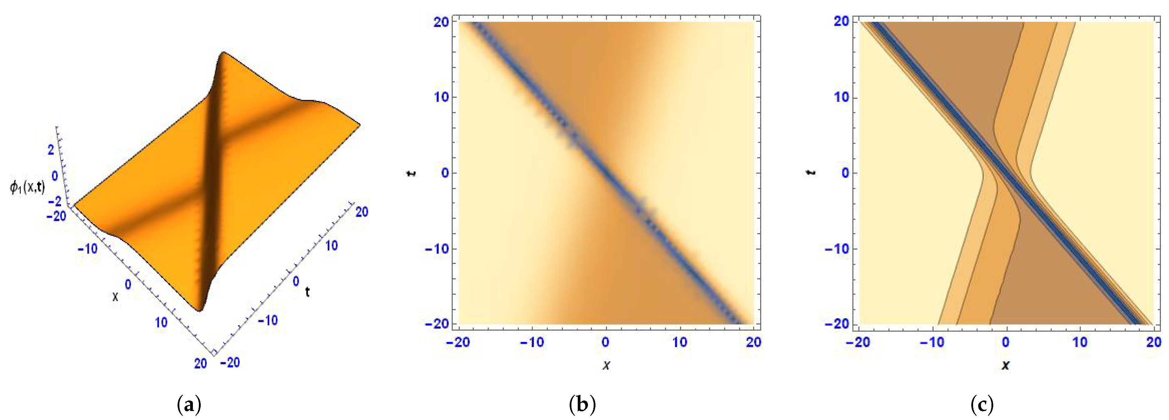
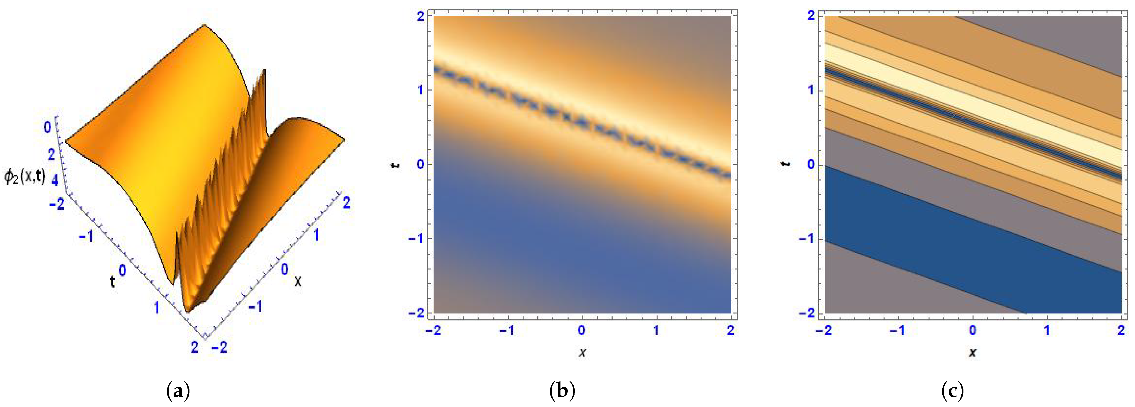
5. Physical Interpretation

This study investigates the lump interaction aspects to a shallow water wave-like equation using the Hirota bilinear approach. One of the top solutions for nonlinear evolution equations has been demonstrated to be the lump solutions. We successfully reported some breather wave, lump-periodic, and two-wave solutions. A breather is a nonlinear wave in physics that has energy concentrated in a focused, oscillating manner. The expectations drawn from the analogous linear system for infinitesimal amplitudes, which lean toward an even distribution of originally localized energy, are in conflict with this. The word “breather” comes from the fact that the majority of breathers oscillate (breathe) in time and are confined in location. Alternatively, oscillations that are localized in time and place are referred to as a break [40]. An expanding dynamic disturbance of one or more values is known as a wave in physics, mathematics, and related subjects. When a wave is periodic, its constituent parts repeatedly oscillate at a given frequency around an equilibrium value. A traveling wave is one where the entire waveform is moving in one direction; in contrast, a standing wave is one where two superimposed periodic waves are moving in opposite directions. A standing wave has nulls in the vibrational amplitude at some locations where the wave amplitude seems reduced or even zero. The standing wave field of two opposing waves known as a wave equation or a one-way wave equation for the dynamics of a single wave in a particular direction are two common ways to explain waves [41]. Under the choice of the good values of the parameters, three-dimensional, density, and contour figures are plotted. Figure 1 and Figure 2 display the collision aspects between lump, exponential function, and singular periodic wave for the breather solutions (6) and (7). Figure 3 and Figure 4 display the collision aspects between lump, exponential function, periodic, and singular periodic waves for the lump-periodic wave solutions (10) and (11). Figure 5 and Figure 6 display the collision aspects between lump, exponential function, periodic, and singular periodic waves for the two-wave solutions (14) and (15).

6. Conclusions

The shallow water wave-like equation has been investigated. The well-known and efficient Hirota bilinear approach was employed to construct several novel solutions to the equation under consideration. Lump-periodic, two-wave, and breather wave solutions were produced as novel forms of results for the governing equation. In the meantime, the figures for these results have been graphed. The propagation properties of the generated solutions are illustrated in the plotted figures using the contour and three-dimensional plots. The results reveal that the appropriate physical quantities and attributes of nonlinear waves are related to the parameter values. The findings may be applied to a wide range of areas to assist readers in better comprehending difficult physical elements. The equation under consideration agreed with the attained solutions.

References

1. Abdel-Khalek, S. Nonautonomous complex wave solutions to the (2+1)-dimensional variable-coefficients nonlinear Chiral Schrodinger equation. Results Phys. 2020, 19, 103604. [Google Scholar] [CrossRef]
2. Yusuf, A.; Sulaiman, T.A.; Khalil, E.M. Construction of multi-wave complexiton solutions of the Kadomtsev-Petviashvili equation via two efficient analyzing techniques. Results Phys. 2021, 21, 103775. [Google Scholar] [CrossRef]
3. Khan, K.; Akbar, M.; Mohd, N.H. The modified simple equation method for exact and solitary wave solutions of nonlinear evolution equation. ISRN Math. Phys. 2013, 2013, 146704. [Google Scholar] [CrossRef]
4. Xu, X.; Zhu, N. Global well-posedness for the 2D Boussinesq equations with partial temperaturedependent dissipative terms. J. Math. Anal. Appl. 2018, 466, 351–372. [Google Scholar] [CrossRef]
5. Gala, S.; Ragusa, M.A. Logarithmically improved regularity criterion for the Boussinesq equations in Besov spaces with negative indices. Appl. Anal. 2016, 95, 1271–1279. [Google Scholar] [CrossRef]
6. Gala, S.; Guo, Z.; Ragusa, M.A. A remark on the regularity criterion of Boussinesq equations with zero heat conductivity. Appl. Math. Lett. 2014, 27, 70–73. [Google Scholar] [CrossRef]
7. Bianca, C.; Pappalardo, F.; Motta, S.; Ragusa, M.A. Persistence analysis in a Kolmogorov-type model for cancer-immune system competition. AIP Conf. Proc. 2013, 1558, 1797–1800. [Google Scholar] [CrossRef]
8. Jaradat, H.M.; Alquran, A.; Syam, I. A reliable study of new nonlinear equation: Two-mode Kuramoto-Sivashinsky. Int. J. Appl. Comput. Math. 2018, 4, 64. [Google Scholar] [CrossRef]
9. Jaradat, I.; Alquran, M.; Ali, M. A numerical study on weak-dissipative two-mode perturbed Burgers’ and Ostrovsky models: Right-left moving waves. Eur. Phys. J. Plus 2018, 133, 164. [Google Scholar] [CrossRef]
10. Jaradat, I.; Alquran, M.; Momani, S.; Biswas, A. Dark and singular optical solutions with dual-mode nonlinear Schrodinger’s equation and Kerr-law nonlinearity. Optik 2018, 172, 822–825. [Google Scholar] [CrossRef]
11. Alquran, M.; Jaradat, I. Multiplicative of dual-waves generated upon increasing the phase velocity parameter embedded in dual-mode Schrodinger with nonlinearity Kerr laws. Nonlinear Dyn. 2019, 96, 115–121. [Google Scholar] [CrossRef]
12. Jaradat, H.M.; Al-Shara, S.; Awawdeh, F.; Alquran, M. Variable coefficient equations of the Kadomtsev–Petviashvili hierarchy: Multiple soliton solutions and singular multiple soliton solutions. Phys. Scr. 2012, 85, 035001. [Google Scholar] [CrossRef]
13. Alquran, M.; Jaradat, H.M.; Al-Shara, S.; Awawdeh, F. A New Simplified Bilinear Method for the N-Soliton Solutions for a Generalized FmKdV Equation with Time-Dependent Variable Coefficients. IJNSN 2015, 16, 259–269. [Google Scholar] [CrossRef]
14. Jaradat, H.M.; Awawdeh, F.; Al-Shara, S.; Alquran, M.; Momani, S. Controllable dynamical behaviors and the analysis of fractal burgers hierarchy with the full effects of inhomogeneities of media. Rom. J. Phys. 2015, 60, 324–343. [Google Scholar]
15. Ma, W.X.; Qin, Z.; Lu, X. Lump solutions to dimensionally reduced p-gKP and p-gBKP equations. Nonlinear Dyn. 2016, 84, 923–931. [Google Scholar] [CrossRef]
16. Yong, X.; Ma, W.X.; Huang, Y.; Liu, Y. Lump solutions to the Kadomtsev-Petviashvili I equation with a self-consistent source. Comput. Math. Appl. 2018, 75, 3414–3419. [Google Scholar] [CrossRef]
17. Yang, J.Y.; Ma, W.X. Abundant lump-type solutions of the Jimbo-Miwa equation in (3+1)-dimensions. Comput. Math. Appl. 2017, 73, 220–225. [Google Scholar] [CrossRef]
18. Tang, Y.; Tao, S.; Guan, Q. Lump solitons and the interaction phenomena of them for two classes of nonlinear evolution equations. Comput. Math. Appl. 2016, 72, 2334–2342. [Google Scholar] [CrossRef]
19. Yang, J.Y.; Ma, W.X.; Qin, Z. Lump and lump-soliton solutions to the (2+1)dimensional Ito equation. Anal. Math. Phys. 2018, 8, 427–436. [Google Scholar] [CrossRef]
20. Ma, W.X. Lump-type solutions to the (3+1)-dimensional Jimbo-Miwa equation. Int. J. Nonlinear Sci. Numer. Simul. 2017, 17, 355–359. [Google Scholar] [CrossRef]
21. Ma, W.X. Lump solutions to the Kadomtsev-Petviashvili equation. Phys. Lett. A 2015, 379, 1975–1978. [Google Scholar] [CrossRef]
22. Yang, J.Y.; Ma, W.X. Lump solutions to the BKP equation by symbolic computation. Int. J. Mod. Phys. B 2016, 30, 1640028. [Google Scholar] [CrossRef] [Green Version]
23. Kauo, D.J. The lump solutions and the Backlund transformation for the three-dimensional three-wave resonant interaction. J. Math. Phys. 1981, 22, 1176–1181. [Google Scholar]
24. Zhang, H.Q.; Ma, W.X. Lump solutions to the (2+1)-dimensional Sawada-Kotera equation. Nonlinear Dyn. 2017, 87, 2305–2310. [Google Scholar] [CrossRef]
25. Chen, S.T.; Ma, W.X. Lump solutions to a generalized Bogoyavlensky-Konopelchenko equation. Front. Math. China 2018, 13, 525–534. [Google Scholar] [CrossRef]
26. Ma, W.X. A search for lump solutions to a combined fourth order nonlinear PDE in (2+1)-dimensions. J. Appl. Anal. Comput. 2019, 9, 1319–1332. [Google Scholar] [CrossRef]
27. Ma, W.X.; Zhou, Y.; Dougherty, R. Lump-type solutions to nonlinear differential equations derived from generalized bilinear equations. Int. J. Mod. Phys. B 2016, 30, 1640018. [Google Scholar] [CrossRef]
28. Zhao, H.Q.; Ma, W.X. Mixed lump-kink solutions to the KP equation. Comput. Math. Appl. 2017, 74, 1399–1405. [Google Scholar] [CrossRef]
29. Yusuf, A.; Sulaiman, T.A.; Inc, M.; Bayram, M. Breather wave, lump-periodic solutions and some other interaction phenomena to the Caudrey–Dodd–Gibbon equation. Eur. Phys. J. Plus 2020, 135, 563. [Google Scholar] [CrossRef]
30. Sulaiman, T.A.; Yusuf, A.; Atangana, A. New lump, lump-kink, breather waves and other interaction solutions to the (3+1)dimensional soliton equation. Commun. Theor. Phys. 2020, 72, 085004. [Google Scholar] [CrossRef]
31. Sulaiman, T.A.; Yusuf, A. Dynamics of lump periodic and breather waves solutions with variable coefficients in liquid with gas bubbles. Waves Random Complex Media 2021, 1–14. [Google Scholar] [CrossRef]
32. Sulaiman, T.A.; Yusuf, A.; Alquran, M. Dynamics of optical solitons and nonautonomous complex wave solutions to the nonlinear Schrodinger equation with variable coefficients. Nonlinear Dyn. 2021, 104, 639–648. [Google Scholar] [CrossRef]
33. Wang, K.J.; Si, J. Investigation into the Explicit Solutions of the Integrable (2+1)—Dimensional Maccari System via the Variational Approach. Axioms 2022, 11, 234. [Google Scholar] [CrossRef]
34. Wang, K.J. Traveling wave solutions of the Gardner equation in dusty plasmas. Results Phys. 2022, 33, 105207. [Google Scholar] [CrossRef]
35. Wang, K.J.; Wang, G.D. Exact traveling wave solutions for the system of the ion sound and Langmuir waves by using three effective methods. Results Phys. 2022, 35, 105390. [Google Scholar] [CrossRef]
36. Wang, K.J. Abundant exact soliton solutions to the Fokas system. Optik 2022, 249, 168265. [Google Scholar] [CrossRef]
37. Wang, K.J.; Wang, G.D.; Shi, F. Abundant exact travelıng wave solutıons to the local fractıonal (3+1)-dimensional Boiti–Leon–Manna–pempinelli equation. Fractals 2022, 30, 2250064. [Google Scholar] [CrossRef]
38. Wei, M.; Cai, J. The Exact Rational Solutions to a Shallow Water Wave-Like Equation by Generalized Bilinear Method. J. Appl. Math. Phys. 2017, 5, 715–721. [Google Scholar] [CrossRef] [Green Version]
39. Vreugdenhil, C.B. Numerical Methods for Shallow-Water Flow, Water Science and Technology Library; Springer: Dordrecht, The Netherlands, 1986. [Google Scholar]
40. Ablowitz, M.J.; Kaup, D.J.; Newell, A.C.; Segur, H. Method for solving the sine-Gordon equation. Phys. Rev. Lett. 1973, 30, 1262–1264. [Google Scholar] [CrossRef]
41. Chakravorty, P. What Is a Signal? [Lecture Notes]. IEEE Signal Process. Mag. 1982, 35, 175–177. [Google Scholar] [CrossRef]
Figure 1. (a) Three-dimensional, (b) density, and (c) contour images of (6) under the values ϑ 0 = 6 , ϑ 1 = 0.75 , γ 1 = 3.5 .
Mathematics 10 02805 g001
Figure 2. (a) Three-dimensional, (b) density, and (c) contour images of (7) under the values ϑ 0 = 7 , γ 1 = 9.55 , ϑ 1 = 0.471 .
Mathematics 10 02805 g002
Figure 3. (a) Three-dimensional, (b) density, and (c) contour images of (10) under the values ϑ 5 = 1 , τ 3 = 18.5 .
Mathematics 10 02805 g003
Figure 4. (a) Three-dimensional, (b) density, and (c) contour images of (11) under the values ϑ 3 = 3.14 , τ 2 = 18.28 .
Mathematics 10 02805 g004
Figure 5. (a) Three-dimensional, (b) density, and (c) contour images of (14) under the values δ 1 = 1 , δ 2 = 2 , c 1 = 1.1 , c 4 = 2 .
Mathematics 10 02805 g005
Figure 6. (a) Three-dimensional, (b) density, and (c) contour images of (15) under the values δ 1 = 0.5 , c 2 = 5.65 , c 1 = 1.1 , c 3 = 17.2 .
Mathematics 10 02805 g006
Publisher’s Note: MDPI stays neutral with regard to jurisdictional claims in published maps and institutional affiliations.