Abstract
With the complicated geology of vein deposits, their irregular and extremely skewed grade distribution, and the confined nature of gold, there is a propensity to overestimate or underestimate the ore grade. As a result, numerous estimation approaches for mineral resources have been developed. It was investigated in this study by using five machine learning algorithms to estimate highly skewed gold data in the vein-type at the Quartz Ridge region, including Gaussian Process Regression (GPR), Support Vector Regression (SVR), Decision Tree Ensemble (DTE), Fully Connected Neural Network (FCNN), and K-Nearest Neighbors (K-NN). The accuracy of MLA is compared to that of geostatistical approaches, such as ordinary and indicator kriging. Significant improvements were made during data preprocessing and splitting, ensuring that MLA was estimated accurately. The data were preprocessed with two normalization methods (z-score and logarithmic) to enhance network training performance and minimize substantial differences in the dataset’s variable ranges on predictions. The samples were divided into two equal subsets using an integrated data segmentation approach based on the Marine Predators Algorithm (MPA). The ranking shows that the GPR with logarithmic normalization is the most efficient method for estimating gold grade, far outperforming kriging techniques. In this study, the key to producing a successful mineral estimate is more than just the technique. It also has to do with how the data are processed and split.
1. Introduction
Since it is one of the earliest stages of a mining operation, the resource estimate is critical in feasibility studies and mine preparation [1,2]. Incorrect resource estimation approaches can have negative impacts, potentially resulting in a ±50% grade estimate error [3]. Hence, choosing the optimum technique with the most effective output for a vein-type deposit is crucial for the deposit’s financial analysis.
However, traditional approaches frequently result in the overvaluation of uneconomic deposits and the undervaluation of payable deposits [4]. Hence, the mining industry has embraced geostatistics to evaluate mineral resource estimations for several decades. Geostatistics methods give reliable tools for comprehensively simulating mineral deposits. Furthermore, various estimating approaches may derive block estimates from the variogram model of the deposit and fit a standard model. On the other hand, the variogram is used in kriging to show the correlation between geological distance and Euclidean distance and weights to aid in estimating unsampled data [5]. Thus, this technique merely examines spatial continuity as the primary issue, in contrast to traditional methods. Still, the failure of variogram modeling, which occurs because of the non-stationarity and normalcy of the data, remains one of the biggest problems with using geostatistics to this day.
Because of the advancements in computer technology and modernism, various machine learning algorithms (MLAs) have been developed as a substitute method for estimating ore grades. Thus, resource estimation has gained appeal among experts as a trustworthy approach, one of several computational model tools. Many studies have attempted to estimate the grade of various mineralizations by using multiple machine learning applications. For example, artificial neural networks (ANNs) [6,7,8,9], adaptive neuro fuzzy inference system (ANFIS) [10], random forest (RF) [11], and Gaussian process (GP) [11,12], support vector machines (SVM) [13,14] k-nearest neighbors (kNN) [15], and combined kNN–ANN methods [2] are the most popularly used algorithms. There have also been some studies that employ machine learning and deep learning approaches to identify the mineral grade and potential anomalies, according to the following publications: [16,17,18]. So, MLAs are becoming more popular, especially in noisy data, such as the kind seen in vein deposits, because of their flexibility and capability to integrate nonlinear correlations between input and output data [19,20]. Moreover, there are no assumptions about any variable or relationship relating to the spatial variation of mineralization [21,22,23]; this is a fundamental advantage. No convincing evidence exists to support the superior effectiveness of one strategy over the other. The advantage of MLAs over the conventional kriging approach has been proved in several applications [23,24]. On the other hand, [25] found that MLAs’ approaches were no better than classic geostatistical techniques.
The estimation issue is particularly challenging in the vein deposits, where the distribution of gold is often relatively inhomogeneous and displays abrupt variations because of the nuggety nature of gold. It results in a highly skewed distribution, which significantly affects the number of blocks whose grades diverge from the actual grade of the deposit [26]. The mineral is concentrated in a few irregularly scattered areas, which causes a substantial change in the statistical parameters and the experimental variogram when outlier datasets are present [27]. So, in order to produce an accurate estimate, the outlier must be capped, and the distribution should be much more controlled [1]. Another thing also essential to consider while inducing appropriate predictors from this is the sparsity of the data and the inhomogeneous distribution of the samples available for learning [28].
Numerous grade value prediction studies use data randomly divided into training and testing subsets, omitting to account for the samples’ inhomogeneous distributions. So, to avoid biased or skewed subsets caused by random data selection, according to the present investigation, this is accomplished by using an integrated data segmentation method that incorporates the marine predators algorithm (MPA) method and divides the data into two equal subsets: training and testing. This enhanced strategy produces a better outcome in data distribution while also making the prediction issue more realistic. The MPA method is modern and has proven to be highly efficient in optimization when compared to its counterparts, and this paper is the first attempt to apply it to mineral estimation [29]. To improve network training performance and minimize substantial differences in the dataset’s variable ranges on the predictions, it is recommended that data vectors be normalized [30]. Therefore, two methods were chosen, namely z-score and logarithmic normalization. This technique guaranteed that the statistical data distribution at each input and output remained uniform, allowing for more accurate estimates.
In this research, to improve the estimate of highly skewed gold data in the vein-type, firstly preprocessed by two normalization approaches (z-score and logarithmic), divided into two equal subsets using an integrated data segmentation with the marine predators algorithm (MPA) method. Then five different machine learning algorithms were applied, and they were compared to two traditional geostatistical approaches (ordinary and indicator kriging). This study gave a novel perspective on choosing the optimum technique for gold prediction and emphasized the critical relevance of preprocessing the data, which is reflected in the model’s performance. Based on the results, the best approach for estimating gold values in vein deposits will be presented as a state-of-the-art strategy.
2. Methods Used
Here are the methods for ore grade estimate approaches used in this study, including geostatistical techniques and machine learning algorithms, which are presented in detail.
Machine learning (ML) and kriging are often referred to as estimation methods based on the input data’s features and weights. In kriging, the estimates are made by multiplying the grades at the sampled locations, which are called “input features” (xi), by the weights (wi). The ML estimate, shown by xi, can be made with any relevant data collected at the sampling point. The ML weights wi are figured out using optimization that uses the known values. Kriging weights are based on a variogram model where the X, Y, and Z data positions are in relation to the estimation location. The estimate is calculated by multiplying the data by the weights. In ML, unlike in kriging, known values at the X, Y, and Z are used to set the weights, which are then used to make an estimate.
ML does not need the assumption of stationarity in estimates; yet ML is a data-driven approach and a kind of regression; as a result, data are not reproduced. This is because ML is a data-driven method. Although kriging is a model-driven estimating method that reproduces data in their original locations, it is necessary for kriging to assume stationarity, which is not always true.
2.1. Geostatistical Technique
2.1.1. Ordinary Kriging
Ordinary kriging (OK) treats mean value like an unknown parameter, allowing for more robustness if the regionalized variable has a mean value, which is locally consistent but globally spatially changing [31]. OK, the estimator, is a suitable method for ore control and reserve/resource estimate technique and is the geostatistical approach chosen most often; therefore, it was selected for this research. OK serves a unique function since it is suitable with a stationary model; it only includes the variogram and is ultimately the most frequently utilized form of kriging [32]. Kriging aims to estimate values for a regionalized variable at a given location, (Zk) Z* (x0), using the current values in the vicinity, Z(xi). Specified locations are given a weighting coefficient (λi) that indicates the effect of specific data on the final estimate value at the selected grid node. The ordinary kriging estimator is:
2.1.2. Indicator Kriging
As Journel (1983) proposed, the indicator kriging is a nonparametric technique for the probability estimate of more than one particular threshold value, Zk, within spatial data [33]. The first step in utilizing the kriging indicator (IK) is to convert it into indicators [1]; this is established by coding the grade above and below a given threshold by zeros and ones. The explanation is the binomial coding of data in either 1 or 0, subject to its connection with the specified cut-off value, Zk [34]. For a given value, Z(x):
Models of indicator variogram are needed for an estimate after data transformation. The indicator variogram looks for significant variances within which a range of interest or influence is identified for each variable. A variance of the indicator may help to find the crucial variance (sill).
2.2. Machine Learning Algorithms in Resource Prediction
Five ML algorithms (GPR, SVR, DTE, FCCN, and K-NN) were used in this study. These algorithms were chosen because they do not require any assumptions, are well-established and robust, and model non-linear relationships.
2.2.1. Gaussian Process Regression (GPR)
As non-parametric techniques in the Bayesian approach to machine learning, Gaussian processes may be used to supervise learning issues, such as regression and classification as well as unsupervised learning issues. The reason they were non-parametric is that, rather than attempting to match the parameters of a specified basis function, generalized linear models (GPs) instead attempt to infer how all the measured data are interrelated. In statistics, a Gaussian process (GP) is described as a collection of random variables having the feature that the joint distribution of any subset of the collection is a joint Gaussian distribution. The GPR-based system has several practical advantages over other supervised learning algorithms, including flexibility, the ability to provide uncertainty estimates, and the ability to learn noise and smoothness parameters from training data. It also works well on small datasets and can provide uncertainty measurements for the predictions [35]. It can be directed from training data to approximate the intrinsic nonlinear connection in any dataset; as a result, it can be used for continuous variable prediction, modeling, mapping, and interpolation [36]. This characteristic makes it appropriate for estimating the grade of ore.
where m(x) = E[f(x)] is the mean function at input x, and k(x; x′) = E[(f(x) − m(x))(f(x′) − m(x′))T] is the covariance function that denotes the dependence between the function values for different input points x and x′.
F(x)~GP (m(x), k(x, x′))
The covariance function is commonly referred to as the kernel of the Gaussian process and implicitly specifies smoothness, periodicity, stationarity, and other model properties. As shown in Equation (4), a simple zero mean and a squared exponential covariance function are employed in Gaussian process regression (GPR).
where r is equal (|x − x′|2/l2) and σf and l are hyper-parameters, which affect the GP algorithm’s performance in a significant way. Where σf denotes the model noise, while the ‘l’ parameter is the length scale. Regardless of the input parameters’ closeness, the covariance between them is near; nevertheless, the covariance decreases exponentially with increasing distance. In the GPR rational quadratic, several covariance/kernel functions may be used to adjust the performance. The predictive distribution model may be produced by conditioning the training data. This is provided by
The average predication can be estimated from the following equation
And the variance prediction may be calculated as
where, covariance matrices K(X, X) and K(X*, X*) are used to represent the covariance matrix of the training and testing datasets, respectively. The vector of covariance between testing and all training observations is denoted by k(x*), t is the joint normalcy of training goal value and is provided by , and X is the joint normalcy of training observation and is given by . IN is the identity matrix of size N × N. It can be shown from the preceding equations that the mean prediction linearly combines the observed target. The variance was independent of the observed target and only dependent on the observed inputs. One characteristic of a Gaussian distribution is that it has this property.
2.2.2. Support Vector Regression (SVR)
Support vector regression is a non-parametric technique that analyses the data for classification, regression, and prediction analysis. It is one of the supervised learning models with related learning algorithms. Researchers have been paying close attention to artificial intelligence approaches in recent years, which is not surprising. In 1990, Vepnayk introduced and demonstrated their capacity to predict difficulties with nonlinear systems [37]. This approach shows significant power in extending and dealing with noise and a lack of data, as shown by the outcomes [38,39].
Support vector regression (SVR) models are like linear regression models, employing a linear function to approximate the regression function. Whereas linear regression seeks to minimize the squared error, which may be significantly affected by a single observation out of phase with the general trend, SVR seeks the so-called insensitive loss function, represented by Equation (8). One of the primary motivations for using SVR is to reduce outliers’ impact on the regression model. An error threshold is used when considering how each data point contributes to the overall loss. The data points of residuals that fall below this threshold may not add to the overall loss.
SVR uses a penalty term for evaluating the parameters of the model. It is possible to describe the objective function in its whole may be represented as Equation (9).
For a given data point, it may show that the prediction function is
The dot product may be substituted by a kernel function κ(xi, x), which represents the dot product in higher dimensions and, as a result, captures the non-linear relationships in the data.
Despite their complexity, SVR models are adaptable and somewhat resilient in the face of outliers and sparse data. SVR can handle linear and non-linear regression problems using various kernel functions. Despite its many advantages, the SVR has certain drawbacks, such as the lack of a probabilistic approach to predictions, and the kernel function must meet the criterion of being a positive definite continuous symmetric function [39].
2.2.3. Decision Tree Ensemble (DTE)
The decision tree is a well-known machine learning technique that gives decision-makers a simple way to analyze and interpret the data. Even though decision trees can be useful for regression problems and classification problems, the latter application is where their popularity lies. The most frequent method for including decision trees in regression models is to use an ensemble strategy. This investigation uses the regression bagging ensemble approach to predict the resource estimation technique.
Decision trees are non-parametric models that perform a series of simple tests for each case. They move through a binary tree structure until they achieve a leaf node (decision) at the end. Because of the enormous prediction variation, the decision tree algorithm is unstable when dealing with high-dimensional input. It is possible to address this challenge by constructing an ensemble of decision trees from the bagged data samples gathered. Ensemble approaches combine several decision trees to get more accurate prediction outcomes. An ensemble model is often used in order to create a strong learner from several weak ones. Both Bagging and Boosting, which provide distinct results but may improve precision and accuracy while reducing the chance of an error, describe the process.
Breiman (1996) came up with the bagging approach, which is also called “bootstrap aggregation”. It may improve the prediction process in regression models by reducing the variation in predictions. An ensemble regression is a type of regression algorithm that combines the results of several base regressions to arrive at the desired final result (regression process). Each base regressor in the ensemble method, such as a regression decision tree or any other regressor, is trained or learned with a subset of the total training data. The training subsets are selected randomly using a method called replacement. Then, the estimation process is performed on every subset, and the total prediction is made by integrating the sub-samples regression averages. This leads to a significant decrease in the variance because of the combining procedure [40]. Consequently, the regression, or the predicting of a new instance, is based on the highest possible number of votes by the base regressors during the final regression process.
2.2.4. Fully Connected Neural Network (FCNN)
FCNNs are constructed of many layers of neurons that each have an input layer, a few hidden layers as well as an output layer. Each layer has neurons that connect to the neurons in the next layer. During the transition between layers, the matrix multiplication process is performed, which assigns a weight to each input feature. Each neuron then produces the total of weighted feature values and transmits them to a non-linear activation function, which outputs the sum of weighted feature values. The activation function output is passed to the next layer. In the model, the activation function causes the neuron to be activated and for the model to be non-linear. The mathematical representation of a fully connected neural network is as follows [41]:
fFCNN: = x ↦ y
x signifies the input vector variable with Nin length, and y denotes the output vector variable with Nout length. The hidden layers, numbered from i = 1, 2,..., Nhl with Nhl designing as the total number of hidden layers, are the primary building component of a fully connected neural network. The mathematical object in the ith hidden layer is indicated as h(i), where Nnpl is the number of neurons in each layer. The feedforward computing technique is the calculation of vectors in a step-by-step manner, which may state mathematically as:
x ↦ h(1) ↦ h(2) ↦ ⋯ ↦ h(Nhl) ↦ y
Despite the benefits that deep learning models have over standard machine learning models, they are sometimes over-parameterized, necessitating the use of large data. Due to data scarcity and sparsity, deep learning algorithms cannot predict material characteristics accurately. Furthermore, deep learning models are challenging to comprehend owing to a lack of pre-defined model structure a complicated hierarchy of layers and neuron activation.
The piecewise continuous nature of the function in Equation (12) necessitates establishing a minimum of two hidden layers within FCNNs, each containing smooth activation functions or a layer that includes both smooth and non-smooth activation functions [42,43]. This is necessary to achieve satisfactory fitting results. This study uses the non-smooth activation function as the tanh activation function to get the desired result. The activation functions are expressed in terms of the following Equation (13):
Tanh: f(x) = (1 − e−2x)/(1 + e−2x)
2.2.5. K-Nearest Neighbors (K-NN)
The K-NN technique is often considered a straightforward way of analyzing multidimensional data. Although this approach is simple, it is also beneficial compared to many other ways, since it allows the user to generalize based on a few training sets [44]. It is one of the earliest and most uncomplicated learning strategies, since it is based on pattern recognition and categorization of previously unidentified items, and it can be employed for classification or regression [45]. KNN regression uses a local average to estimate the output variable value, whereas KNN classification seeks to predict which class the output variable belongs to. Fix and Hodges (1989) and Cover and Hart (1967), for example, characterized it as a nonparametric technique for discriminant analysis (lazy similarity learning algorithm). The term “k-neighbors” of a sample refers to the k samples nearest to the sample in terms of distance from the sample. It is possible to generate a regression model’s output as a weighted average of each of the k nearest neighbors, with each neighbor’s weight being inversely proportional to how far it is from the input data. When using the K-NN methodology, it is critical to choose the appropriate number of KNNs since the number of K-NNs selected may significantly affect the prediction accuracy of the method. Using low values of k will lead to over-fitting (high variance), while using excessive values of k will cause very biased models. Although there are several distance functions, Euclidean is frequently utilized. Wilson and Martinez (2000) provide the following definition of the Euclidean distance function.
where, x and y represent the query point, respectively, while m denotes the number of input variables (attributes).
The algorithm predicts the new instance by comparing it to the training data. The comparison is based on the distance metric between the new model and the previously stored training data. Computed distance values are then put in ascending order. Lastly, the kNN regressor’s prediction is the average of the first k numbers of the neighbors closest to the test instance. The KNN approach has many appealing characteristics. When compared to linear regression, this technique may provide much better results. It performs well on datasets with limited features and a few variables. No optimization or training is needed beyond the selection of K-NNs and the distance measure used in the analysis. The approach uses local information and may provide decision limits that are highly nonlinear and very adaptable. As a result, the process has a high computational and memory cost since it requires scanning all the data available points (i.e., samples) to discover the most similar neighbors. Calculating distances gets increasingly difficult when dealing with large datasets with several dimensions. Despite these drawbacks, the approach is widely used because of its implementation simplicity and the characteristics mentioned above [46]. In the current study, the K-NN is applied to predict the resource of gold, the k parameter is set to 3 as the best value obtained by experiments.
2.3. Marine Predators Optimization Algorithm (MPA)
The optimization approaches have been remarkable in recent years. They are more efficient in dealing with the various optimization fields, including machine learning and feature selection, than other existing techniques [47]. There are different optimization algorithms, i.e., meta-heuristics algorithms, such as evolutionary algorithms (e.g., genetic algorithms (GA)) [48] and swarm intelligence (SI) techniques (e.g., particle swarm optimization (PSO) [49]). The marine predators algorithm (MPA) is a nature-inspired optimization algorithm [29]. This optimization algorithm simulates the marine creatures’ behavior in searching for prey; these inherited steps are employed to solve and optimize the problem and reach the optimal solution. The MPA algorithm uses foraging strategies known as Lévy and Brownian motions in ocean predators as well as an optimum encounter rate policy for the biological interactions that take place between predators and prey. The starting position of an MPA may be characterized as follows:
where rand is a random vector with values between 0 and 1 that are uniformly distributed, the lower and higher bounds of the variables are denoted by the notation XLower and Xupper, respectively.
X0 = XLower + rand (Xupper − XLower)
Top natural predators are thought to be more skilled foragers, according to the survival of the fittest concept. As a result, the most appropriate solution is designated as a top predator to create the elite matrix. This matrix is used to search for and locate prey based on the prey’s location.
where XI is the best predator vector out of n simulations used to construct the elite matrix (E), d represents the number of dimensions, and n is the variable that specifies the number of candidates.
There is also a matrix known as prey, which has the same dimensions as elite, and the predators adjust their locations based on it. The initialization process results in the generation of the first prey, from which the strongest individual (the predator) selects and creates the elite. This is an illustration of the prey:
where Xi,j represents the ith prey’s jth dimension. Specifically, the optimization approach is linked to these matrices.
Predator-and-prey interactions are detailed in three parts of the MPA:
- Prey is faster than a predator.
- The predator is faster than the prey.
- Predator and prey have similar speeds.
The MPA algorithm has been employed to optimize various problems in COVID-19 image classification [50] or image segmentation processes [51]. This motivated us to utilize the MPA algorithm for the train/test split dataset to get a balanced data distribution over the train and test dataset.
2.4. Model Validation and Performance Evaluation
K-fold cross-validation (CV), a commonly used validation approach, was applied in this work throughout the performance assessment of the training dataset and hyper-parameters optimization. The training data are randomly divided into k folds for the k-fold CV. The training is carried out on (K-1) folds, with the residual one fold being utilized to confirm the training results. K iterations of the training validating procedure are required (with various folds of the validating fold) to accurately forecast the entire training set. For this study, the value of k was chosen to be five because of computational efficiency.
The vein deposit data were divided into two distinct groups: training and testing. The learning procedure is done using training datasets in any ANN architecture, while testing datasets confirm the model’s performance. Even though cross-validation is widely regarded as a method of evaluating model performance, it might lead to over-fitting when applied to actual data [22,52].
For the Quartz Ridge vein-type, the applicability of geostatistics-based models and machine learning-based models was evaluated. The performance of machine learning approaches was also examined using the same prediction dataset utilized in the kriging techniques to make the predictions. It was decided to use multiple accuracy measures to evaluate the model’s overall performance.
(i) The correlation coefficient (R) indicates how strongly two variables are related when they change; (ii) The coefficient of determination (R2) assesses model fitting accuracy. It is defined as the ratio of actual data variance to estimated value variance, and the linear fit equation characterizes it. It is deemed acceptable to have a model with an R2 of at least 55%, less than 30% is thought suspicious, and over 75% is considered outstanding [53]; (iii) The root mean square error (RMSE) represents the residuals’ standard deviation (prediction errors). A commonly used measure of the differences between predicted or estimated values and observed values is ideally where the RMSE would be zero; (iv) the mean bias error (MBE), which illustrates if a model under- or overestimates the grades, is also an important measure to consider. Positive signs imply underestimating, while negative signs indicate overestimation in this situation; (v) the mean absolute error (MAE) is a statistic that quantifies the mean absolute variation between actual and predicted values; and (vi) mean squared error (MSE) takes into consideration both the bias and the error variance but is also more susceptible to outliers than the mean absolute error.
The accuracy and precision are represented by the RMSE, MBE, MAE, and MSE. When these metrics are lower in value, the expected grades are closer to the actual grades [54]. The skill value (Equation (18)) test is utilized to analyze further the model performance, which is a similar technique to that employed by [14,25]. MBE, MAE, R2, and RMSE were used in this technique since the skill values may be subjectively determined; these tools were selected for this strategy.
Skill value = MBE + MAE + RMSE + 100 (1 − R2)
3. Case Study Area
Since ancient times, the eastern wilderness of Egypt has been renowned as a gold mining area. The Arabian-Nubian Shield (is one of many sections of the African Continental Crust that formed during the Pan-African Orogeny) Neoproterozoic basement rocks contain gold in approximately 100 sites throughout the whole region covered by Precambrian basement rocks [55,56,57]. The majority of these deposits were found and mined by the ancient Egyptians (4000 B.C.), who also discovered and exploited the top portions in numerous locations [58,59]. According to recent reports, the Sukari gold mine (SGM) is Egypt’s first large-scale and modernized gold production operation. The gold mineralization and accompanying mineral alteration are extensively distributed throughout the shield’s geological history. The overwhelming bulk of the gold resources in Egypt are of the orogenous vein-type [60]. The dominant host rocks are granites, mafic to ultramafic rocks, metavolcanic and volcanoclastic rocks, and metasediments [61]. The primary transport fluids are thought to be metamorphic hydrothermal fluids, while the primary source of gold is thought to be mafic/ultramafic ophiolitic rocks [62,63].
The Quartz Ridge Vein Deposit
Quartz Ridge is a new field in the Central Eastern Desert (CED) (24°56′ N, 34°45′ E) about 5 km east of the Sukari gold mine within a 160 km2 rectangular concession area. It is important to mention that the Sukari gold mine contains resources of more than 14.3 million ounces of gold, giving greater attention to the neighboring undiscovered prospects [64]. The Quartz Ridge area is one of the most promising areas in the Sukari concession. As a result, it receives more attention to existing reserves and, as a result, generates a higher income and return. The vein region is the only part of the study area being investigated. The dominant lithology in the research region is gabbro-diorite (intermediate plutonic rocks) with equigranular texture, which may be observed as massive and sheared; this host rock is impacted by shear, which provides a higher gold assay than a quartz vein (Figure 1) [65]. The quartz vein extends along the strike for about 500 m, with a 1.5 m.
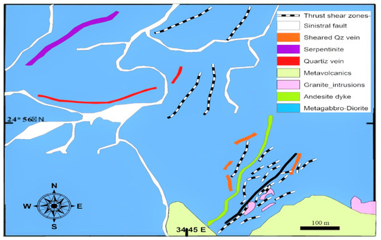
Figure 1.
The geologic map of the Quartz Ridge prospect area, including the studied QR vein in the black rectangle.
The mineralization is contained in quartz veins across NE-trending shear zones and their associated altered wall rocks, according to the geological context of the research region. As for the vast majority of gold deposits in Egypt, in geochemical and geological studies of the area that were recently published, all evidence confirms gold in the region.
4. Results and Discussion
4.1. Data Analysis and Descriptive Statistics
This case study is based on a gold mineralization deposit of the vein. This deposit is entirely virgin because no previous mining in this specific region occurred. There are 124 exploration boreholes done in the vein region, the boreholes not in the regular grid, total 1079 samples, with an average drilling spacing of approximately 20 m. Samples from the boreholes were taken at varying intervals. The samples are collected from a variety of lithological types. Diamond drilling (DD) holes and reverse circulation (RC) drill holes have been used to sample the orebody over the last few years. Sample coordinates (easting, northing, and elevation), sample length, rock type, and gold grade were tested. A variety of software packages, including Microsoft Excel, SPSS, and Geovia Surpac, were utilized to evaluate the data. In this research, Surpac was used to do modeling, statistical and geostatistical analysis, and estimate gold.
Statistical analyses on raw data have been performed, and the results are presented below (Table 1). In accordance with this statistical analysis, the raw samples showed a statistically significant amount of grade variation, with a mean and standard deviation of 0.525 and 3.671, respectively. The coefficient of variation for the gold deposit is 6.997, indicating a significant degree of variance [66]. It demonstrates that there may be a few outliers (up to 93.12 ppm), a significant variance (13.479), and potential estimation errors. According to a visual examination of the histogram graph, as seen in Figure 2, the drilling dataset consists mainly of low-grade values, with just a few extremely high-grade values in the data. The histogram reveals that the dataset contains over one population and that the distribution is significantly positively skewed. When dealing with skewed distributions, a slew of difficulties might occur. This disparity results in an imbalance in the frequencies of sample values, which biases the estimate. Therefore, a lognormal distribution was established for the gold assay results, and the original data values were changed by taking the logarithm of the gold value (Figure 2). This kind of skewness is quite widespread in the distribution of gold deposits, and it may be seen in several locations. It reveals that the gold distribution varies from the normal distribution in several ways [67].

Table 1.
Summarizes the statistical data on gold grade (Raw vs. Composited data).
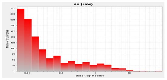
Figure 2.
Logarithmic histogram of gold distribution.
Borehole samples have been examined and have been found to have an uneven length. It is critical to use equal support (volume) samples for all the samples in estimating. For this reason, the data were composited in equivalent size [68]. Samples data were constrained and composited to 1 m in length to improve relevant statistical analysis comparable to the mean depth range in one run—established a minimum distance of 75% of a composite size. The deposit of the Quartz Ridge vein has a few very high values, so to manage the outliers, many techniques for determining a top cut value use concepts, such as histogram, confidence interval, percentile, from this equation (Mean + 2 S.D.), and experience [1,69].
Furthermore, in resource evaluation, the top-cut procedure lacks defined criteria and is susceptible to analyst judgment [70]. As a result, an upper cut-off grade of 10 ppm was applied to the data before estimating all grades greater than 10 ppm; five samples were identified as outliers. Samples were composited at one meter in length and capped at 10 ppm. The summary statistics of gold composites are shown in Table 1. When the raw data are compared to the composites after capping, the ratio of maximum to mean is 20 times lower in the raw data.
4.2. Variographic Study
A variogram and covariance functions are computed in the initial phase of using kriging spatial interpolation techniques. The second stage is to evaluate a location that has not been sampled.
Variograms are one of the most successful strategies for demonstrating spatial coherence in geostatistical estimates [31,32]. Geostatistical estimates are based on the spatial structure of the data. An experimental variogram is ideal for the examination of local data, and it is created based on the fundamental measurement of heterogeneity [33]. Variograms are measurements of spatial correlation, and they can identify anisotropy if the size of such a spatial correlation differs with direction. To determine the anisotropy of a spatial variation, an experimental variogram must be constructed in several directions. As a result, the anisotropic direction is established using variogram modeling in two or three orientations. Anisotropy is divided into geometric anisotropy and also zonal anisotropy, in response to differences in the range or domain of the variograms. Anisotropy can be used to estimate and simulate underground conditions based on their orientation and dimensions.
4.2.1. Grade Variography Analysis for OK
A variography was initially carried out in this study to perform the resource estimates. First, variogram analysis is constructed to confirm grade continuity using the variographic range and find the studied element’s spatial correlation. Its use allows the identification of the mineralization’s main directions and the subsequent creation of variograms in these directions. Deutsch and Journel (1998) proposed that the experimental variograms were based on three orthogonal directions. Each experimental variogram was constructed using the mineralization envelope composite values. Establishing an omnidirectional variogram before constructing a directional variogram was necessary to achieve a suitable sill variance offered by the deposit.
Three different types of variograms were constructed for the Quartz Ridge vein: omnidirectional, downhole, and directional. Table 2 shows the parameters for each of them. The results of the modeling of the omnidirectional variogram (Figure 3) revealed that the exponential model well represented the typical continuity for a grade of gold. With the spherical model, the downhole variogram demonstrates distinct spatial features and moderates variability.
Table 2.
Variogram models for estimation with their characteristics.
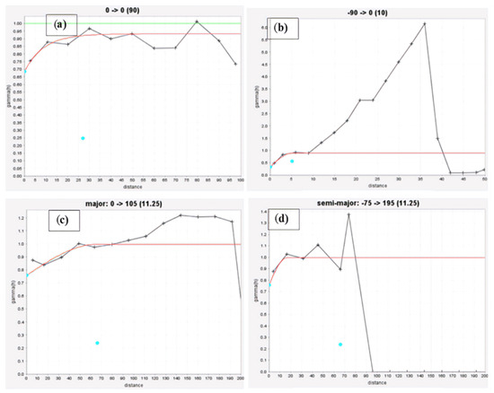
Figure 3.
Au experimental variogram and modeling for (a) omnidirectional, (b) downhole, (c) major, and (d) semi-major directional variograms.
Besides improving knowledge of the deposit, the directional variogram model made it possible to look for anisotropies in the sample. After many trials and errors, the variogram with the best summary statistics was finally selected. After constructing these models, the kriging method was used to estimate grades in an area not sampled. The directional variogram model was fitted using a typical spherical model in Figure 3, and the parameters used to construct the directional variogram are listed in Table 2. All orientations had different mineralization continuity based on variogram models. As a result, the mineralization was considered to be anisotropic.
The fitted spherical model made a somewhat high nugget effect, with such a dependence ratio of C0/(C0 + C1) of approximately 56 percent, indicating relatively average variance and moderate continuity as seen in Table 2 (a percentage of the nugget to total semivariance of between 25% and 75% shows moderate spatial dependence) [71,72].
4.2.2. Indicator Variography Analysis and Modeling
In order to assess the spatial continuity, a set of four cut-offs were utilized for the directional indicator variograms, namely 0.3, 0.6, 0.9, and 1.5 ppm. The mine’s stated mining cut-offs are based on waste, low, and high-grade ores. The lag spacing and angular tolerance are chosen adequately to acquire a sufficient number of samples. Figure 4 shows the experiment-based variograms and the models that fit them, while Table 3 shows the parameters.
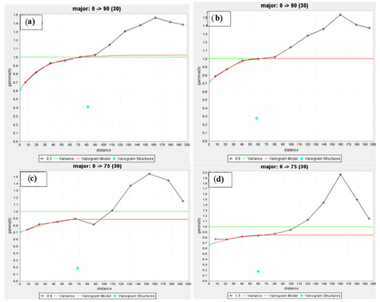
Figure 4.
Indicator variogram modeling of data at four cut-offs in the main direction (a) 0.3, (b) 0.6, (c) 0.9, and (d) 1.5 ppm, respectively.
Table 3.
Indicator variogram parameters for four specified cut-offs.
When modeling the variograms at the three different orientations, it was determined that a spherical structure was appropriate for modeling the variograms at the three different cut-offs (0.6, 0.9, and 1.5 ppm). However, at 0.3 parts per million (ppm), the model was exponential, and it reported the largest range of influence (81.3 m) and the lowest nugget effect (0.612 ppm2) of any of the four cut-offs, as shown in Table 3. Consequently, it directly impacted the result and was associated with the lowest percentage for the relative nugget effect (0.6), showing relatively large variation and moderate continuity.
The significant proportions of spatial variability resulting from the nugget effect show a weak spatial correlation structure in the deposit across the studied region—the value of the range changes in various directions, demonstrating geometric anisotropy. The fitted spherical model (0.9 and 1.5 ppm cut-offs) had a high nugget effect, with a dependence ratio of (sill/nugget) of approximately 79 percent, as seen in Table 3. This percentage was more significant than 75%, which shows high variance and weak spatial dependence [71,72].
4.3. Block Modeling for Resource Estimation
Kriging gives the best estimation because it leads to the lowest standard error, the lowest confidence interval, and the highest confidence (lowest risk) [73]. The deposit was well-suited to ordinary kriging as an estimated approach because the procedure worked well enough on historical models.
Block modelling of the deposit is carried out to make resource estimation more accurate. When a parent block was chosen, it had the following characteristics: 20 m E × 20 m N × 5 m RL. These characteristics were chosen based on the geometry of the geological, the strategy of exploiting the spacing between the boreholes, and the compositing. The parent block covered the interpreted mineralization domain. Sub-blocking was used to guarantee that the volume representation was appropriate [74]. Table 4 depicts the size of the blocks used in modelling and the coordinates boundaries. Based on the geological information available about this deposit, an average specific gravity of 2.67 was applied to all blocks for tonnage calculations. In this study, the grade of every block was estimated by using ordinary kriging from the vein domain.
Table 4.
Shows the parameters and extents of the block model.
Indicator kriging estimates were computed using ordinary kriging with parameters derived from the indicator semi-variogram models and sample search ellipsoid, which were defined based on the variography and data spacing.
4.4. Preparing Data for Machine Learning Approaches and Training Specifications
Several different machine learning models, including GPR, SVR, DT Ensemble, FCNN, and K-NN, have been used to estimate the grade of the ore. These models have all been shown to evaluate the ore grade successfully. Specifically, for grade estimation, spatial coordinates (north (y), east (x), and (z)) and gold concentration may be utilized as the input and output vectors for the prediction of grade, respectively. The machine learning technique was implemented in a commercial software program in the MATLAB environment.
Using an integrated strategy that incorporates data segmentation [14] and the marine predators algorithm (MPA), which serves as an optimization algorithm, the dataset is separated into training and testing subsets [75]. As part of this process, the original dataset is split into three prime segments (Seg 1, Seg 2, and Seg 3), categorized as low, medium, and high-grade gold concentrations. These prime segments are then subdivided into sub-prime segments; this division is carried out based on a visual analysis of the dataset histogram plot. The data segmentation strategy is shown in a representative diagram in Figure 5.
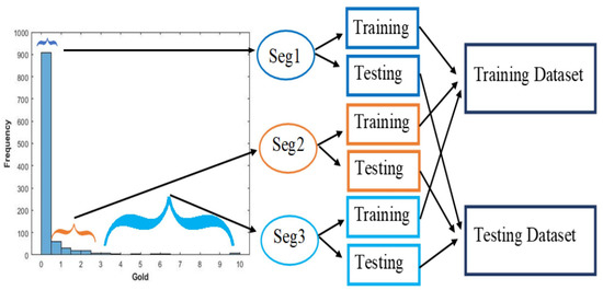
Figure 5.
Data segmentation of gold values for training and testing based on the histogram plot.
The optimization method MPA is used to map these three data segments, namely Seg 1, Seg 2, and Seg 3, into newly created training and testing datasets. Furthermore, the mapping is carried out in such a way that the mean and standard deviation of the results from the training and testing sets are similar, where the training dataset comprises 80 percent of the samples, with 863 samples, and the testing dataset comprises 20 percent of the samples, with 216 samples. In addition, the histogram plots of the original dataset, the training dataset, and the testing dataset are shown in Figure 6, demonstrating the similarity in gold concentrations between the training and testing datasets, respectively.
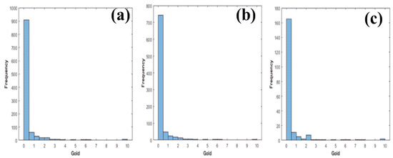
Figure 6.
Histogram plot of gold values for (a) entire dataset (b) training dataset (c) testing dataset.
In order to improve network training performance, it is recommended that data vectors be normalized. This guaranteed that the statistical distribution of data at each input and output remained uniform, allowing for more accurate estimates [8,76]. After trial and error with differing normalizing techniques, two preprocessing techniques can be employed for the variables: z-score normalization and logarithmic normalization were selected because they performed well compared to the other ways. These strategies were used to minimize the impact of wide variations in the dataset’s variable ranges on the predictions.
The normalized observations data were randomly separated into two datasets: a training set (which was used to iteratively construct a mapping function between both the output and the desired output) and a test set (which was used to evaluate the mapping function) (for network validation). Randomly dividing datasets into training and testing sets makes sense when the datasets are significant and have an accepted nugget effect. A network’s performance is assessed based on its generalization, which refers to how it performs on unobserved data.
The hyper-parameters have been optimized to get the optimal parameters for each applied ML algorithm. The optimization algorithm tries to find the suitable parameters for each ML method (Table 5). It generates a set of initial parameters and evolves them to reach the best parameter values according to the prediction problem. There are several hyper-parameters to consider, such as training iterations, learning rate, number of hidden units, and network depth. This is a time-consuming and challenging operation. Moreover, another significant challenge and limitation in using machine learning methods is re-conducting the analysis with the same dataset and changing no parameters. Some differences may be observed in the outcomes because the program randomly determines the training and testing datasets. Bayesian optimization is a helpful method for optimizing models, and it was chosen and used in this study [77]. A heuristic technique is used to determine the optimal network, which is capable of avoiding over-fitting in terms of network performance. For neural network training, a limited-memory Broyden–Fletcher–Goldfarb–Shanno (LBFGS) numerical optimization technique [78] was employed to maximize the network learning rate. However, decision tree ensembles using the bag and LSBoost approaches are used instead. In the Gaussian process regression, the rational quadratic kernel is used. In support vector regression, the Gaussian kernel is used.
Table 5.
Parameter settings for the applied machine learning algorithms.
4.5. Comparative Performance of the All Models
To ensure that the results of data analysis are as accurate as possible, it is vital to choose a normalization method that influences the ranking issue, the range of normalized values, achieving a uniform optimization aspect across criteria, and the validity of outcomes. The results of a normalization procedure directly influence the outcomes of the analyses to be done [30,79,80]. Here is a discussion of the results of the first normalization, z-score normalization, and a comparison of those with the outcomes of the linear and non-linear kriging procedures. Table 6 shows the results of the models run on the test dataset for predicting the gold content of the vein deposits. The results show that all of the machine learning and kriging algorithms performed almost equally well on the dataset.
Table 6.
Results from geostatistical analysis and the effectiveness of machine learning models for predicting gold content (testing dataset, z-score normalization technique).
As shown in Figure 7 and Figure 8, the values of the correlation coefficient (R) for GPR, SVR, DTE, FCNN, K-NN, IK, and OK were 0.21, 0.18, 0.076, 0.064, 0.138, 0.304, and 0.445, respectively. Compared to other models, the OK model has the highest correlation coefficient value; on the other hand, the FCNN model has the lowest correlation coefficient value. Similarly, the R2 values for the GPR, SVR, DTE, FCNN, K-NN, IK, and OK are 0.185, 0.160, 0.065, 0.055, 0.119, 0.09, and 0.20, respectively. This is a strong indication of the OK and GPR’s mediocre performance when compared to other models. The FCCN had the lowest performance of all the different kinds of models tested in this dataset. It was observed that the R2 values for the geostatistical techniques OK and IK had deficient performance when it comes to gold grade in the previous studies. In this study, the gold in the vein deposit has high skewness as well as high coefficients of variation, which may explain why the model performs so poorly, especially when compared to the findings of variogram modeling, which showed that every variogram model had a very high nugget/sill component, making the R2 values reasonable. Notably, the R2 values show that ordinary kriging performs somewhat better than ML models. Nevertheless, every model’s R2 value is suboptimal, coming in at a number lower than 0.5. There are two significant reasons for this. The first, and most importantly, is the weak spatial correlation of the gold dataset inside the research region and the fact that the data are extremely skewed. Another explanation shown in this study is that the normalization approach had a significant influence only when the output variable produced using ML was numeric.

Figure 7.
Scatterplots comparing actual vs. expected values for ordinary kriging (left) and indicator kriging (right).
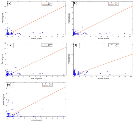
Figure 8.
After z-score normalization, actual vs. projected values for (a) GPR, (b) SVR, (c) DTE, (d) FCNN, and (e) K-NN for testing data.
Similarly, the RMSE value with the GPR technique was the lowest at 0.901 and was followed by the DTE approach with a value of 0.914, whereas the IK model had the highest RMSE value of 1.266, making it the most accurate of all the models (Table 6). Statistical analysis shows that the SVR algorithm performs poorly compared to the other ML algorithms. In addition, the resulting plot in Figure 8 (the training and testing plot for SVR) indicates that the SVR algorithm is unable to fit or understand the relationship between the data after using the z-score normalization strategy. The modeling techniques had modest prediction biases, except for the K-NN model, which had a high positive error bias. The only overestimated model was the K-NN model, which had a mean error of 0.936. The FCNN model had the lowest tendency to overestimate among the models tested, with a mean error of −0.006.
In order to make it easier to compare the outcomes, a summary measure of performance was developed. It enables the approaches to be ranked in terms of their overall performance as well as their performance on the test set. It is important to note that the skill value (Equation (18) described above) should be lower for better techniques and more remarkable for inferior ways [14,25].
As shown in Table 7, the skill values and ranks for the various methods used on the prediction dataset were presented. The accuracy ranking of seven methods from low to high in the following order: OK, GPR, SVR, K-NN, IK, DTE, and FCNN. The large variety in the R2 is responsible mainly for the disparity in skill values. In the end, the OK model is placed first since it has the lowest skill value of all the models tested in this study (in light of the fact that there is little difference between OK and GPR methods). As a result, the ordinary kriging technique of geostatistics was used to estimate the resource estimate of the Quartz-Ridge vein deposit. The OK model outperforms both the IK and the machine learning models. Other models’ generalization capabilities are outperformed by the OK technique, which also delivers superior accuracy in prediction than that of other methods. Similar observations have been made elsewhere [25], and our data are compatible with them.
Table 7.
Model performances rated according to their overall skill value.
Instead of using z-score normalization, the variable preprocessing technique uses logarithmic normalization. Logarithmic preprocessing is often used to minimize the disparities between values; in this case, it applies to all the features’ values to get the desired result. The training, testing datasets, and hyperparameters are the same as in the z-score normalization. The further point is that both the training and test data kept their mean and standard deviation values from the normalization technique, essentially the same as those in the original data. Machine learning models were tested on a dataset with R2 values in Figure 9 to prove their correctness (GPR, SVR, DTE, FCNN, and K-NN).
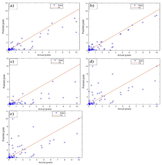
Figure 9.
After logarithmic normalization, actual vs. projected values for (a) GPR, (b) SVR, (c) DTE, (d) FCNN, and (e) K-NN for testing data.
When comparing both methodologies, Table 6 shows significant variances from Table 8. The logarithmic normalization outperforms the z-score normalization in terms of performance, and it has been shown to enhance the model while also producing the most accurate representation of the data. The GPR model is the best in the test dataset only for ML models using the Z-score normalization technique. Moreover, the GPR model has the best performance and efficiency when using the logarithmic strategy and outperforms all other models, including geostatistical methods. Meanwhile, the FCCN model maintained the same poor performance and ranking in both comparison methodologies. As a result, as represented by FCCN, deep learning cannot be used to assess the high skewness of the gold vein’s resources.
Table 8.
Model performance for predicting gold content (logarithmic strategy testing dataset).
It is evident that after using the logarithm technique, the R2 values have quadrupled, with the majority of models having values of more than 55%–75%, indicating exceptional performance [53]. As a result, adopting the logarithmic normalizing approach may increase prediction performance and provide an advantage over other methods. Nevertheless, the value of utilizing multiple normalization methods is not taken into consideration by researchers. When the approach of z-score normalization was used to estimate the gold content in this research, the unstable behavior of the SVR model was observed. On the contrary, the findings indicated the SVR model outperformed the logarithm technique by 70% for R2, and it is deemed the second-best model after GPR. This emphasizes the significance of the chosen normalization strategy.
In Table 7 and Table 9, based on the overall skill values, the rank of the machine learning methods is shown to have changed from OK, GPR, DTE, K-NN, IK, FCNN, and SVR, respectively, for the z-score normalization to GPR, SVR, K-NN, DTE, and FCNN, respectively, for the logarithmic normalization. According to our research, the logarithmic approach has superior performance and efficiency. The algorithmic methodology is used in machine learning methods to outperform traditional geostatistical techniques. The prediction achieved using GPR was superior to those produced by all the other combined approaches. These results are supported by those obtained using the GPR model, which has been discussed before [11].
Table 9.
Model performances rated according to their overall skill value.
There are two reasons to expect that the outcomes will be unsatisfactory because of the use of ordinary kriging: first, because it generates locally linear estimates, and second, because of the smoothing effect. Smoothing happens everywhere in the model that is produced using kriging because each grid point uses a weighted average of the samples that are located nearby. An attempt was made to model the deposit using nonlinear machine learning algorithms. Using the z score normalization resulted in similarly unsatisfactory results; hence, consideration was given to a new tactic, explicitly applying the logarithmic normalization. This investigation into Au prediction showed that ML with logarithmic normalization performed significantly better than kriging the model. The study found the method itself is not the most critical factor in producing the most accurate and desirable results when estimating the grade of highly skewed, complex geology; instead, data processing plays the most crucial role.
Based on the findings detailed in Table 6, Table 7, Table 8 and Table 9 and Figure 7, Figure 8, Figure 9 and Figure 10, it is clear that the regression method that uses a Gaussian process yields the best results overall. Figure 10 provides a visual representation of the quality of the various approaches’ estimates for gold grade values in the western section of the Quartz Ridge vein-type. These predictions were made using a variety of different methodologies. In conclusion, the GPR approach is superior to the kriging method in every way. This is accomplished by supposing a parametrized model of the covariance function and using a Bayesian technique (maximizing the marginal probability) to estimate the optimum values for these parameters. The Bayesian procedure achieves accurate results. Because of this, GPR uses both local and global data. The study found the method itself is not the most critical factor in producing the most accurate and desirable results when estimating the grade of highly skewed, complex geology; instead, data preprocessing plays the most crucial role.
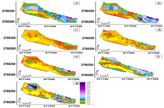
Figure 10.
The spatial distributions of estimated Au values for the western section of the quartz vein, looking north, applying each of the following methodologies: (a) OK, (b) IK, (c) GPR, (d) SVM, (e) DTE, (f) FCNN, and (g) K-NN.
5. Conclusions
Accurate grade prediction is crucial for effective project execution throughout the exploration and exploitation stages of the mining process. One of the most challenging mineralization forms to estimate and utilize economically is mineralization with a significant nugget effect, such as gold-bearing veins. This issue was highly apparent in this study region; hence, the research focused on estimating the vein-type deposit and applying it to similar deposits.
This work applied five machine learning algorithms (GPR, SVR, DTE, FCCN, and K-NN). The machine learning algorithm’s input variables were north, east, and elevation, while the output variable was the gold grade. Choosing the best normalizing method was important because of the data’s sparsity and skewness. In this study, both z-score and logarithmic normalization were used. In order to make a model and test it, two statistically equivalent subsets were created by combining data segmentation and the marine predators algorithm (MPA). This strategy efficiently provides subsets of data that are statistically similar.
At the end of the study, MLA’s accuracy was compared to geostatistical approaches. These models may be ranked by different statistical metrics based on skill levels. This research showed that the R and R2 values improved by more than three times over at least for all models, while an acceptable relative increase in the RMSE and MAE values was observed, and the overall ranking is superior to the models that used the logarithmic method. Consequently, the GPR approach outperformed all geostatistical and other machine learning methods evaluated, and it had the lowest skill value of all the strategies investigated. In addition, the SVR model may predict gold ore sometimes. The deep learning FCCN model cannot be relied on to be accurate. This study was used to make improvements while preprocessing and dividing the data. In particular, this was reflected in selecting a robust technique that can accurately estimate the gold value in a vein deposit, ensuring a high degree of reliability and generalizability of similar deposits.
Author Contributions
Conceptualization, M.M.Z., S.C., M.A.M. and K.M.S.; methodology, M.M.Z.; software, M.M.Z., M.A.M. and K.M.S.; validation, M.M.Z., M.A.M. and S.C.; formal analysis, M.M.Z.; data curation, M.M.Z.; writing—original draft preparation, M.M.Z.; writing—review and editing, M.M.Z., S.C., J.Z., F.F., A.A.K. and M.A.M.; visualization, M.M.Z.; supervision S.C.; funding acquisition, S.C. All authors have read and agreed to the published version of the manuscript.
Funding
This study was supported by National Natural Science Foundation of China (No. 52074169, 52174159).
Acknowledgments
The authors would like to express their gratitude to Centamin PLC for providing the case study dataset. For their enthusiastic support and insightful comments during the manuscript review, the authors are grateful to Mohamed Bedair, Bahaa Gomah, Recky F. Tobing, Bahram Jafrasteh, and Samer Hmoud. The authors are also grateful for the valuable comments from the academic editor and the anonymous reviewers, which helped us improve our manuscript.
Conflicts of Interest
The authors declare no conflict of interest.
References
- Sinclair, A.J.; Blackwell, G.H. Applied Mineral Inventory Estimation; Cambridge University Press: Cambridge, UK, 2006; ISBN 1139433598. [Google Scholar]
- Kaplan, U.E.; Topal, E. A new ore grade estimation using combine machine learning algorithms. Minerals 2020, 10, 847. [Google Scholar] [CrossRef]
- Dominy, S.C.; Noppé, M.A.; Annels, A.E. Errors and uncertainty in mineral resource and ore reserve estimation: The importance of getting it right. Explor. Min. Geol. 2002, 11, 77–98. [Google Scholar] [CrossRef]
- Haldar, S.K. Mineral Exploration: Principles and Applications; Elsevier: Amsterdam, The Netherlands, 2018; ISBN 0128140232. [Google Scholar]
- Allard, D.J.-P.; Chilès, P. Delfiner: Geostatistics: Modeling Spatial Uncertainty; John Wiley & Sons: Hoboken, NJ, USA, 2013. [Google Scholar]
- Samanta, B.; Ganguli, R.; Bandopadhyay, S. Comparing the predictive performance of neural networks with ordinary kriging in a bauxite deposit. Trans. Inst. Min. Metall. Sect. A Min. Technol. 2005, 114, 129–140. [Google Scholar] [CrossRef]
- Chatterjee, S.; Bhattacherjee, A.; Samanta, B.; Pal, S.K. Ore grade estimation of a limestone deposit in India using an artificial neural network. Appl. GIS 2006, 2, 1–2. [Google Scholar] [CrossRef]
- Li, X.L.; Xie, Y.L.; Guo, Q.J.; Li, L.H. Adaptive ore grade estimation method for the mineral deposit evaluation. Math. Comput. Model. 2010, 52, 1947–1956. [Google Scholar] [CrossRef]
- Singh, R.K.; Ray, D.; Sarkar, B.C. Recurrent neural network approach to mineral deposit modelling. In Proceedings of the 2018 4th International Conference on Recent Advances in Information Technology (RAIT), Dhanbad, India, 15–17 March 2018; pp. 1–5. [Google Scholar] [CrossRef]
- Tahmasebi, P.; Hezarkhani, A. Application of Adaptive Neuro-Fuzzy Inference System for Grade Estimation; Case Study, Sarcheshmeh Porphyry Copper Deposit, Kerman, Iran. Aust. J. Basic Appl. Sci. 2010, 4, 408–420. [Google Scholar]
- Jafrasteh, B.; Fathianpour, N.; Suárez, A. Comparison of machine learning methods for copper ore grade estimation. Comput. Geosci. 2018, 22, 1371–1388. [Google Scholar] [CrossRef]
- Das Goswami, A.; Mishra, M.K.; Patra, D. Adapting pattern recognition approach for uncertainty assessment in the geologic resource estimation for Indian iron ore mines. In Proceedings of the 2016 International Conference on Signal Processing, Communication, Power and Embedded System (SCOPES), Paralakhemundi, India, 3–5 October 2016; pp. 1816–1821. [Google Scholar] [CrossRef]
- Patel, A.K.; Chatterjee, S.; Gorai, A.K. Development of a machine vision system using the support vector machine regression (SVR) algorithm for the online prediction of iron ore grades. Earth Sci. Inform. 2019, 12, 197–210. [Google Scholar] [CrossRef]
- Dutta, S.; Bandopadhyay, S.; Ganguli, R.; Misra, D. Machine learning algorithms and their application to ore reserve estimation of sparse and imprecise data. J. Intell. Learn. Syst. Appl. 2010, 2, 86. [Google Scholar] [CrossRef]
- Mlynarczuk, M.; Skiba, M. The application of artificial intelligence for the identification of the maceral groups and mineral components of coal. Comput. Geosci. 2017, 103, 133–141. [Google Scholar] [CrossRef]
- Sun, T.; Li, H.; Wu, K.; Chen, F.; Zhu, Z.; Hu, Z. Data-Driven Predictive Modelling of Mineral Prospectivity Using Machine Learning and Deep Learning Methods: A Case Study from Southern Jiangxi Province, China. Miner 2020, 10, 102. [Google Scholar] [CrossRef]
- Xiong, Y.; Zuo, R.; Carranza, E.J.M. Mapping mineral prospectivity through big data analytics and a deep learning algorithm. Ore Geol. Rev. 2018, 102, 811–817. [Google Scholar] [CrossRef]
- Rodriguez-Galiano, V.; Sanchez-Castillo, M.; Chica-Olmo, M.; Chica-Rivas, M. Machine learning predictive models for mineral prospectivity: An evaluation of neural networks, random forest, regression trees and support vector machines. Ore Geol. Rev. 2015, 71, 804–818. [Google Scholar] [CrossRef]
- Bishop, C.M. Neural Networks for Pattern Recognition; Oxford University Press: Oxford, UK, 1995; ISBN 0198538642. [Google Scholar]
- Chatterjee, S.; Bandopadhyay, S.; Machuca, D. Ore grade prediction using a genetic algorithm and clustering Based ensemble neural network model. Math. Geosci. 2010, 42, 309–326. [Google Scholar] [CrossRef]
- Koike, K.; Matsuda, S.; Suzuki, T.; Ohmi, M. Neural Network-Based Estimation of Principal Metal Contents in the Hokuroku District, Northern Japan, for Exploring Kuroko-Type Deposits. Nat. Resour. Res. 2002, 11, 135–156. [Google Scholar] [CrossRef]
- Samanta, B.; Bandopadhyay, S.; Ganguli, R.; Dutta, S. Sparse data division using data segmentation and kohonen network for neural network and geostatistical ore grade modeling in nome offshore placer deposit. Nat. Resour. Res. 2004, 13, 189–200. [Google Scholar] [CrossRef]
- Zhang, X.; Song, S.; Li, J.; Wu, C. Robust LS-SVM regression for ore grade estimation in a seafloor hydrothermal sulphide deposit. Acta Oceanol. Sin. 2013, 32, 16–25. [Google Scholar] [CrossRef]
- Das Goswami, A.; Mishra, M.K.; Patra, D. Investigation of general regression neural network architecture for grade estimation of an Indian iron ore deposit. Arab. J. Geosci. 2017, 10, 80. [Google Scholar] [CrossRef]
- Afeni, T.B.; Lawal, A.I.; Adeyemi, R.A. Re-examination of Itakpe iron ore deposit for reserve estimation using geostatistics and artificial neural network techniques. Arab. J. Geosci. 2020, 13, 657. [Google Scholar] [CrossRef]
- Arroyo, D.; Emery, X.; Peláez, M. Sequential simulation with iterative methods. In Geostatistics Oslo 2012; Springer: Berlin/Heidelberg, Germany, 2012; pp. 3–14. [Google Scholar]
- Machado, R.S.; Armony, M.; Costa, J.F.C.L. Field Parametric Geostatistics—A Rigorous Theory to Solve Problems of Highly Skewed Distributions. In Geostatistics Oslo 2012; Springer: Berlin/Heidelberg, Germany, 2012; pp. 383–395. [Google Scholar]
- Samanta, B.; Bandopadhyay, S.; Ganguli, R. Data segmentation and genetic algorithms for sparse data division in Nome placer gold grade estimation using neural network and geostatistics. Explor. Min. Geol. 2002, 11, 69–76. [Google Scholar] [CrossRef]
- Faramarzi, A.; Heidarinejad, M.; Mirjalili, S.; Gandomi, A.H. Marine Predators Algorithm: A nature-inspired metaheuristic. Expert Syst. Appl. 2020, 152, 113377. [Google Scholar] [CrossRef]
- Aytekin, A. Comparative analysis of the normalization techniques in the context of MCDM problems. Decis. Mak. Appl. Manag. Eng. 2021, 4, 1–25. [Google Scholar] [CrossRef]
- David, M. Geostatistical Ore Reserve Estimation; Elsevier: Amsterdam, The Netherlands, 2012; ISBN 0444597611. [Google Scholar]
- Rossi, M.E.; Deutsch, C. V Mineral Resource Estimation; Springer Science & Business Media: Berlin/Heidelberg, Germany, 2013; ISBN 1402057172. [Google Scholar]
- Wackernagel, H. Multivariate Geostatistics: An Introduction with Applications; Springer Science & Business Media: Berlin/Heidelberg, Germany, 2003; ISBN 3540441425. [Google Scholar]
- Hawkins, D.M.; Rivoirard, J. Introduction to Disjunctive Kriging and Nonlinear Geostatistics. J. Am. Stat. Assoc. 1996, 38, 337–340. [Google Scholar] [CrossRef]
- MacKay, D.J.C. Gaussian Processes-a Replacement for Supervised Neural Networks, NIPS Tutorial. 1997. Available online: https://citeseerx.ist.psu.edu/viewdoc/summary?doi=10.1.1.47.9170 (accessed on 15 July 2022).
- Firat, M.; Gungor, M. Generalized Regression Neural Networks and Feed Forward Neural Networks for prediction of scour depth around bridge piers. Adv. Eng. Softw. 2009, 40, 731–737. [Google Scholar] [CrossRef]
- Cristianini, N.; Shawe-Taylor, J. An Introduction to Support Vector Machines and Other Kernel-Based Learning Methods; Cambridge University Press: Cambridge, UK, 2000; ISBN 0521780195. [Google Scholar]
- Steinwart, I.; Christmann, A. Support Vector Machines; Springer Science & Business Media: Berlin/Heidelberg, Germany, 2008; ISBN 0387772421. [Google Scholar]
- Tipping, M. Sparse Bayesian Learning and the Relevance Vector Machine. J. Mach. Learn. Res. 2001, 1, 211–244. [Google Scholar]
- Sutton, C.D. Classification and regression trees, bagging, and boosting. Handb. Stat. 2005, 24, 303–329. [Google Scholar]
- Wang, Y.-T.; Zhang, X.; Liu, X.-S. Machine learning approaches to rock fracture mechanics problems: Mode-I fracture toughness determination. Eng. Fract. Mech. 2021, 253, 107890. [Google Scholar] [CrossRef]
- Selmic, R.R.; Lewis, F.L. Neural-network approximation of piecewise continuous functions: Application to friction compensation. IEEE Trans. Neural Netw. 2002, 13, 745–751. [Google Scholar] [CrossRef]
- Sontag, E.D. Feedback Stabilization Using Two-Hidden-Layer Nets. In Proceedings of the 1991 American Control Conference, Boston, MA, USA, 26–28 June 1991; pp. 815–820. [Google Scholar]
- Rokach, L. Pattern Classification Using Ensemble Methods; World Scientific: Singapore, 2009; Volume 75, ISBN 978-981-4271-06-6. [Google Scholar]
- Song, Y.; Liang, J.; Lu, J.; Zhao, X. An efficient instance selection algorithm for k nearest neighbor regression. Neurocomputing 2017, 251, 26–34. [Google Scholar] [CrossRef]
- González-Sanchez, A.; Frausto-Solis, J.; Ojeda, W. Predictive ability of machine learning methods for massive crop yield prediction. SPANISH J. Agric. Res. 2014, 12, 313–328. [Google Scholar] [CrossRef]
- Shrivastava, P.; Shukla, A.; Vepakomma, P.; Bhansali, N.; Verma, K. A survey of nature-inspired algorithms for feature selection to identify Parkinson’s disease. Comput. Methods Programs Biomed. 2017, 139, 171–179. [Google Scholar] [CrossRef] [PubMed]
- Holland, J.H. Genetic algorithms. Sci. Am. 1992, 267, 66–73. [Google Scholar] [CrossRef]
- Kennedy, J.; Eberhart, R.C. A discrete binary version of the particle swarm algorithm. In Proceedings of the 1997 IEEE International Conference on Systems, Man, and Cybernetics, Orlando, FL, USA, 12–15 October 1997; Volume 5, pp. 4104–4108. [Google Scholar]
- Sahlol, A.T.; Yousri, D.; Ewees, A.A.; Al-Qaness, M.A.A.; Damasevicius, R.; Elaziz, M.A. COVID-19 image classification using deep features and fractional-order marine predators algorithm. Sci. Rep. 2020, 10, 15364. [Google Scholar] [CrossRef] [PubMed]
- Elaziz, M.A.; Ewees, A.A.; Ibrahim, R.A.; Lu, S. Opposition-based moth-flame optimization improved by differential evolution for feature selection. Math. Comput. Simul. 2020, 168, 48–75. [Google Scholar] [CrossRef]
- Lu, X.; Zhou, W.; Ding, X.; Shi, X.; Luan, B.; Li, M. Ensemble Learning Regression for Estimating Unconfined Compressive Strength of Cemented Paste Backfill. IEEE Access 2019, 7, 72125–72133. [Google Scholar] [CrossRef]
- Prasad, K.; Gorai, A.K.; Goyal, P. Development of ANFIS models for air quality forecasting and input optimization for reducing the computational cost and time. Atmos. Environ. 2016, 128, 246–262. [Google Scholar] [CrossRef]
- Samanta, B. Radial basis function network for ore grade estimation. Nat. Resour. Res. 2010, 19, 91–102. [Google Scholar] [CrossRef]
- Hume, W.F. Geology of Egypt: The minerals of economic values associated with the intrusive Precambrian igneous rocks. Ann. Geol. Surv. Egypt 1937, 2, 689–990. [Google Scholar]
- Harraz, H.Z. Primary geochemical haloes, El Sid gold mine, Eastern Desert, Egypt. J. Afr. Earth Sci. 1995, 20, 61–71. [Google Scholar] [CrossRef]
- Klemm, R.; Klemm, D. Gold Production Sites and Gold Mining in Ancient Egypt. In Gold and Gold Mining in Ancient Egypt and Nubia; Springer: Berlin/Heidelberg, Germany, 2013; pp. 51–339. [Google Scholar]
- Eisler, R. Health risks of gold miners: A synoptic review. Environ. Geochem. Health 2003, 25, 325–345. [Google Scholar] [CrossRef]
- Helmy, H.M.; Kaindl, R.; Fritz, H.; Loizenbauer, J. The Sukari Gold Mine, Eastern Desert—Egypt: Structural setting, mineralogy and fluid inclusion study. Miner. Depos. 2004, 39, 495–511. [Google Scholar] [CrossRef]
- Khalil, K.I.; Moghazi, A.M.; El Makky, A.M. Nature and Geodynamic Setting of Late Neoproterozoic Vein-Type Gold Mineralization in the Eastern Desert of Egypt: Mineralogical and Geochemical Constraints; Springer: Berlin/Heidelberg, Germany, 2016; pp. 353–370. [Google Scholar] [CrossRef]
- Botros, N.S. A new classification of the gold deposits of Egypt. Ore Geol. Rev. 2004, 25, 1–37. [Google Scholar] [CrossRef]
- Helba, H.A.; Khalil, K.I.; Mamdouh, M.M.; Abdel Khalek, I.A. Zonation in primary geochemical haloes for orogenic vein-type gold mineralization in the Quartz Ridge prospect, Sukari gold mine area, Eastern Desert of Egypt. J. Geochem. Explor. 2020, 209, 106378. [Google Scholar] [CrossRef]
- Kriewaldt, M.; Okasha, H.; Farghally, M. Sukari Gold Mine: Opportunities and Challenges BT—The Geology of the Egyptian Nubian Shield; Hamimi, Z., Arai, S., Fowler, A.-R., El-Bialy, M.Z., Eds.; Springer International Publishing: Cham, Germany, 2021; pp. 577–591. ISBN 978-3-030-49771-2. [Google Scholar]
- Centamin plc Annual Report 2021. Available online: https://www.centamin.com/media/2529/cent-ar21-full-web-secure.pdf. (accessed on 15 July 2022).
- Bedair, M.; Aref, J.; Bedair, M. Automating Estimation Parameters: A Case Study Evaluating Preferred Paths for Optimisation. In Proceedings of the International mining geology Conference, Perth, Australia, 25–26 November 2019. [Google Scholar]
- Vann, J.; Guibal, D.; Harley, M. Multiple Indicator Kriging–Is it suited to my deposit. In Proceedings of the 4th International Mining Geology Conference, Coolum, Australia, 14–17 May 2000. [Google Scholar]
- Davis, J.C.; Sampson, R.J. Statistics and Data Analysis in Geology; Wiley: New York, NY, USA, 1986; Volume 646. [Google Scholar]
- Daya, A.A.; Bejari, H. A comparative study between simple kriging and ordinary kriging for estimating and modeling the Cu concentration in Chehlkureh deposit, SE Iran. Arab. J. Geosci. 2015, 8, 6003–6020. [Google Scholar] [CrossRef]
- Babakhani, M. Geostatistical Modeling in Presence of Extreme Values. Master’s Thesis, University of Alberta, Edmonton, AB, Canada, 2014. [Google Scholar]
- Kim, S.-M.; Choi, Y.; Park, H.-D. New outlier top-cut method for mineral resource estimation via 3D hot spot analysis of Borehole data. Minerals 2018, 8, 348. [Google Scholar] [CrossRef]
- Dunham, S.; Vann, J. Geometallurgy, geostatistics and project value—Does your block model tell you what you need to know. In Proceedings of the Project Evaluation Conference, Melbourne, Australia, 19–20 June 2007; pp. 19–20. [Google Scholar]
- Cambardella, C.A.; Moorman, T.B.; Novak, J.M.; Parkin, T.B.; Karlen, D.L.; Turco, R.F.; Konopka, A.E. Field-scale variability of soil properties in central Iowa soils. Soil Sci. Soc. Am. J. 1994, 58, 1501–1511. [Google Scholar] [CrossRef]
- Vann, J.; Jackson, S.; Bertoli, O. Quantitative kriging neighbourhood analysis for the mining geologist-a description of the method with worked case examples. In Proceedings of the 5th International Mining Geology Conference, Bendigo, Australia, 17–19 November 2003; Australian Inst Mining & Metallurgy: Melbourne, Victoria, 2003; Volume 8, pp. 215–223. [Google Scholar]
- Tercan, A.E.; Sohrabian, B. Multivariate geostatistical simulation of coal quality data by independent components. Int. J. Coal Geol. 2013, 112, 53–66. [Google Scholar] [CrossRef]
- Cuevas, E.; Fausto, F.; González, A. The Locust Swarm Optimization Algorithm BT—New Advancements in Swarm Algorithms: Operators and Applications; Cuevas, E., Fausto, F., González, A., Eds.; Springer International Publishing: Cham, Germany, 2020; pp. 139–159. ISBN 978-3-030-16339-6. [Google Scholar]
- Asadisaghandi, J.; Tahmasebi, P. Comparative evaluation of back-propagation neural network learning algorithms and empirical correlations for prediction of oil PVT properties in Iran oilfields. J. Pet. Sci. Eng. 2011, 78, 464–475. [Google Scholar] [CrossRef]
- Snoek, J.; Larochelle, H.; Adams, R.P. Practical bayesian optimization of machine learning algorithms. Adv. Neural Inf. Process. Syst. 2012, 25. [Google Scholar]
- Byrd, R.H.; Lu, P.; Nocedal, J.; Zhu, C. A Limited Memory Algorithm for Bound Constrained Optimization. SIAM J. Sci. Comput. 1995, 16, 1190–1208. [Google Scholar] [CrossRef]
- Vafaei, N.; Ribeiro, R.A.; Camarinha-Matos, L.M. Normalization techniques for multi-criteria decision making: Analytical hierarchy process case study. In Proceedings of the Doctoral Conference on Computing, Electrical and Industrial Systems, Costa de Caparica, Portugal, 7–9 July 2021; Springer: Berlin/Heidelberg, Germany, 2016; pp. 261–269. [Google Scholar]
- Corazza, A.; Di Martino, S.; Ferrucci, F.; Gravino, C.; Mendes, E. Applying support vector regression for web effort estimation using a cross-company dataset. In Proceedings of the 2009 3rd International Symposium on Empirical Software Engineering and Measurement, Helsinki, Finland, 19–23 September 2009; pp. 191–202. [Google Scholar]
Publisher’s Note: MDPI stays neutral with regard to jurisdictional claims in published maps and institutional affiliations. |
© 2022 by the authors. Licensee MDPI, Basel, Switzerland. This article is an open access article distributed under the terms and conditions of the Creative Commons Attribution (CC BY) license (https://creativecommons.org/licenses/by/4.0/).