Abstract
The contact behavior of a hemisphere pressed by a rigid plane is of great significance to the study of friction, wear, and conduction between two rough surfaces. A flattening contact behavior of an elastic–perfectly plastic hemisphere pressed by a rigid flat is researched by using the finite element method in this paper. This behavior, influenced by different elastic moduli, Poisson’s ratios, and yield strengths, is compared and analyzed in a large range of interference values, which have not been considered by previous models. The boundaries of purely elastic, elastic–plastic, and fully plastic deformation regions are given according to the interference, maximum mean contact pressure, Poisson’s ratio, and elastic modulus to yield strength ratio. Then, a new elastic–plastic constitutive model is proposed to predict the contact area and load in the elastic–plastic range. Compared with previous models and experiments, the rationality of the present model is verified. The study can be applied directly to the contact between a single sphere and a plane. In addition, the sphere contact can also be used to simulate the contact of single asperity on rough surfaces, so the present proposed model can be used to further study the contact characteristics of rough surfaces.
1. Introduction
The elastic–plastic contact behavior between hemisphere and rigid plane is one of the fundamental problems in particle mechanics [1,2], contact mechanics [3,4,5,6,7,8,9], and biomechanics [10]. Mechanical surfaces are microscopically rough. Contact between two rough surfaces can be equivalent to contact between a hemisphere and a rigid flat [11,12,13]. The study of elastic–plastic contact behavior between hemisphere and a rigid flat is of great significance to the analysis of electrical contact [14,15,16,17], friction [18,19], and wear [20,21] between two rough surfaces.
The early contact model only predicted the elastic contact behavior between the hemisphere and the rigid flat. Greenwood and Williamson (GW model) [22] analyzed the pure elastic contact behavior between hemisphere and rigid flat. With the increase of interference, the hemispheres yield, and the contact state changes from pure elastic to elastic–plastic. Based on the Hertz solution [23], the GW model presented the critical normal interference (ωc), critical contact load (Fc), and critical contact area (Ac) formulas for the initial yield of the hemisphere. However, the Poisson’s ratio (ν) effect is ignored in their predicted formulas for these critical contact parameters. Later, Lin and Lin (LL model) [24] and Chang et al. (CEB model) [25,26] improved the GW model and further considered the effect of different ν on these critical contact parameters. In the elastic–plastic contact stage, the contact behavior is highly nonlinear due to the existence of plasticity. Some scholars have predicted the elastic–plastic contact behavior between hemispheres and rigid planes through experiments [27,28]. However, the experimental results only apply to specific materials. Because the finite element method (FEM) can accurately simulate the contact process between hemisphere and rigid flat of different materials, some researchers have analyzed on the elastic–plastic contact behavior between hemisphere and rigid flat based on the FEM [29,30,31,32,33].
Kogut and Etsion (KE Model) [31] analyzed the effect of the ratio of the elastic modulus to yield strength (E/Y) on the elastic–plastic contact behavior in the range of 100 to 1000 based on FEM. They demonstrated that when the dimensionless mean contact pressure (p/Y) reaches its maximum, the contact state changes from elastic–plastic to fully plastic, with the corresponding dimensionless interference (ω/ωc) as a constant value equal to 110. Based on the analysis results, they presented the empirical relationship between the p/Y ratio, dimensionless contact load (F/Fc), dimensionless contact area (A/Ac), and ω/ωc within ω/ωc = 110. By analyzing the hemisphere and rigid plane contact under different Y based on the FEM, Jackson and Green (JG model) [32,33] proposed that the maximum value of p/Y was not the constant value equal to 2.8, which had been predicted by Tabor [34] for different Y. Based on the results, they presented a new model for predicting the elastic–plastic contact parameters. They defined the initial range of elastic–plastic; however, the termination range of elastic–plastic is not clear in their research. Quicksall et al. [35] used FEM to study the elastic–plastic contact behavior of malleable cast iron, aluminum, titanium, copper, and bronze hemispheres with rigid planes. The results were compared with the predicted by the KE and JG models. They showed that the prediction accuracy of the JG model is higher than that of the KE model, but the formula of the JG model is more complex than that of the KE model.
Elastic–plastic is a complex nonlinear behavior. For the large ω/ωc values and different materials, the previous results of fitting may not be accurate enough for small interference or specific materials. Based on the KE and JG models, many scholars analyzed the effect of material properties and contact properties on hemispheric elastic–plastic contact behavior [36,37,38,39]. Brizmer et al. (BK model) [37] analyzed the effect of material properties and contact conditions at the end of elastic deformation in spherical contact. They found that the initial yield of plastic materials always occurred at a point on the axis of symmetry of the hemisphere, while the brittle failure always occurred at the hemisphere contact surface. Shankar and Mayuram (SM model) [38] analyzed the contact behavior between hemisphere and rigid flat under different Y and compared the results with those predicted by KE and JG models. They found that when E/Y is 79.4, the prediction accuracy of previous KE and JG models is poor. Therefore, they improved the JG and KE models and proposed a new hemispheric contact model. Then, they further considered the effect of the tangential modulus (Et) on hemispheric contact behavior [39]. Malayalamurti and Marappan (MM model) [40] analyzed the influence of different hemispherical radii (R) and Y on hemispherical elastic–plastic contact behavior. Based on the analysis results, they proposed an empirical relationship between F/Fc, A/Ac, and ω/ωc. Sahoo and Chatterjee (SC Model) [41,42] used FEM to analyze the elastic–plastic contact behavior between a sphere and a rigid flat under different E, Et, and R. They observed that the hemispheric elastic–plastic contact behavior is similar at different R. They demonstrated that when Et is small, the result is similar to these predicted of the KE model. With the increase of Et, the prediction accuracy of the KE model becomes worse. However, they do not provide a prediction formula. Under different Y and ν, Megalingam and Mayuram (MM model [43]) analyzed the elastic–plastic contact behavior between hemisphere and rigid flat. Then, the effect of Et on the elastic–plastic contact behavior was further considered [44]. They showed that Y and Et have a greater effect on hemispheric elastic–plastic contact behavior than ν. They also presented a formula for calculating F/Fc and A/Ac in the elastic–plastic range. Recently, Gheadnia et al. [45,46,47] analyzed elastic–plastic contact behavior between the deformable hemisphere and the flat using FEM by controlling the yield strength ratio between hemisphere and flat (Y1/Y2). They demonstrated that the elastic–plastic contact behavior is related to the Y1/Y2 ratio.
Due to the complexity of elastic–plastic problems, there is still no closed solution. Although some hemispheric contact models exist, there is still a lack of a model to compare and analyze hemispheric elastic–plastic contact behavior over different E, ν, Y, and large ω/ωc values. In this paper, the elastic–plastic contact behavior of the hemisphere pressed by the rigid flat by E, ν, and Y was analyzed based on FEM. According to ω/ωc, maximum p/Y, ν, and E/Y, the boundaries of elastic, elastic–plastic, and fully plastic deformation regimes were given. A new elastic–plastic constitutive model was proposed to predict the A/Ac and F/Fc in the elastic–plastic range. Compared with the results predicted by previous models and experiments, the rationality of the present model is verified. In Section 2, the critical contact parameters for the initial yield of hemispheres are analyzed. The FE model is presented in Section 3. In Section 4, the empirical formula of hemispheric elastic–plastic contact is demonstrated by curve fitting, and the results are compared with previous models. The conclusions are presented in the last section.
2. Critical Formula
A flattening model of a deformable hemisphere pressed by a rigid flat before and after loading is shown in Figure 1. A uniform downward load (F) is applied to the top of the hemispheres to simulate loading. At a small interference (ω), the contact state is purely elastic. With an increase of interference, the initial yield occurs at the contact subsurface depth z of the hemisphere, marking the end of purely elastic deformation or the inception of elastic–plastic deformation.
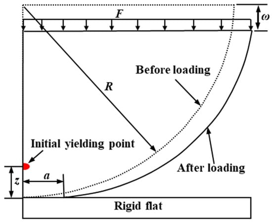
Figure 1.
A flattening model before (dashed line) and after (solid line) loading.
The interference (ω) at the initial yield is called the critical interference, ωc, which is calculated according to the formula provided by Johnson [3] and given by
where E is the equivalent elastic modulus and R is the equivalent radius. ν1, ν2, and E1, E2 are the Poisson’s ratios and elastic moduli of the two materials in contact, respectively. R1 and R2 are the radii of the contact pairs. p0 is maximum Hertzian pressure, which is listed in Table 1.

Table 1.
Summary of maximum contact pressure (p0).
As shown in Table 1, p0 is related to material hardness (H), where H is equal to 2.8 Y predicted by Tabor [34] in the GW model [22], CEB model [26], and LL model [24]. However, this relationship between H and Y, recently pointed out by the JG model [33] and SM model [38], was not the constant value equal to 2.8. In the Green model [32], BK model [37], and JG model, p0 is predicted by using the von Mises yield criterion and the stress field of Johnson, which seems more reasonable than the GW model, CEB model, and LL model. The yield strength coefficient (C) is a function of Poisson’s ratio (ν). It is shown in Figure 2. The critical results of all models are the same at ν = 0.35. For the common materials (0.2 ≤ ν ≤ 0.45), except for the GW model, the critical interference of the JG model, CEB model, Green model, LL model, and BK model are similar.
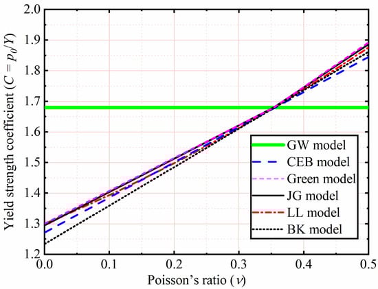
Figure 2.
Yield strength coefficient as a function of Poisson’s ratio.
Considering the above discussion and the meaning of p0, the critical interference is chosen in this study by the JG model and given by
The contact state is purely elastic before the initial yielding of the hemispherical contact (ω < ωc). The contact load (Fe) and the contact area (Ae) can be expressed as
when the interference equals the critical interference (ω = ωc), their critical values can be expressed as
These critical values predict the particular contact parameters at the inception of elastic–plastic deformation. Therefore, they are selected to nondimensionalize the results in all models.
3. Finite Element Model
The finite element model presently used in this paper is similar to the finite element model described by the JG model [33], SM model [38,39], and SC model [41]. The commercial program ANSYS18.2-Workbench was used for modeling and analyzing the contact behavior of a deformable hemisphere pressed by a rigid flat. Due to its axial symmetry, a 2-D model was selected. The hemisphere was modeled by a quarter of a circle (R = 1 mm), while a half-space represented the rigid flat surface. The boundary load was applied, as shown in Figure 3. The nodes of a half-space were fixed in all directions to model the rigid flat. The nodes on the symmetry axis of the hemisphere were fixed in the radial direction to model a half-sphere. The tangent modulus and the friction coefficient were assumed as zero within ANSYS. The von Mises yield criterion was used to define material yield. The present analysis covers a wide range of material properties [48]. As shown in Table 2 and Table 3, the analyzed material properties were divided into two groups. Specifically, the property ranges of the 79.4 ≤ E/Y ≤ 800 and 0.2 ≤ ν ≤ 0.45 were considered. The half-sphere and half-space by PLANE 183 triangle elements were discretized in such a way that there were many elements near the contact edge, as shown in Figure 3. The mesh far from the contact edge became coarser to improve computing speed. The half-sphere and half-space total number of elements was 37,391 and 15,028, respectively. Additionally, their total number of nodes were 75,662, and 33,164, respectively. For the half-sphere, the JG model used a constant mesh of 11,101 elements, the KE model used a maximum of 2944 nodes in total, and the SM model used 9933 elements in total for their analysis. By comparison, the present model mesh was better. There are 2696 two-dimensional three-node surface contact elements, designated as CONTA172 and TARGE169 in ANSYS, to detect the contact behavior of a deformable hemisphere pressed by a rigid flat. The uniform displacement was applied to the bottom section of the hemisphere, and then the contact force was obtained by extracting the reaction force of the node at its bottom. The contact area was calculated by the contact radius, which was obtained by finding the contacting edge. The results compare well with the Hertz elastic solution at ω ≤ ωc. The error between them is less than 2%. In addition, to ensure mesh convergence, the mesh density was iterated twice until the result of each iteration changed by no more than 1%. Due to the material and geometric nonlinearity, the Augmented Lagrange algorithm was adopted, and a large deflection was activated. Additionally, multi-step loading was used to guarantee the solution convergence. The maximum number of substeps in the calculation for very large interference was 15,000. In order to obtain a generalized model, all contact parameters were in dimensionless form, i.e., F/Fc, ω/ωc, p/Y, and A/Ac.
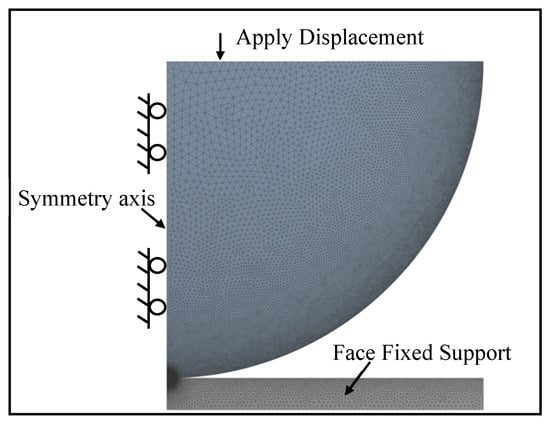
Figure 3.
Finite element mesh and boundary conditions.
Table 2.
Material properties in the first group.
Table 3.
Material properties in the second group.
4. Results and Discussion
4.1. Contact Load
The effects of E and ν shown in Table 2 on F/Fc as a function of ω/ωc were analyzed. Here Y was a constant value equal to 0.25 GPa, while ν were 0.2, 0.3, 0.4, and 0.45. With E ranging from 45 to 200 GPa, corresponding the E/Y ratios ranging from 180 to 800, respectively. Here only the results of ν = 0.2 and 0.45 for E/Y = 180, 280, 400, 600, and 800 were selected and plotted in Figure 4. F/Fc increases with an increasing ω/ωc. For 1< ω/ωc ≤ 110, the results indicate the similarity with the KE model, F/Fc is independent of E and ν of the material. For 110 < ω/ωc ≤ 500, F/Fc decreased with a decreasing E. Moreover, it is clear from Figure 4 that the SM model underestimates F/Fc. The reason of this discrepancy is that it is valid only for the E/Y ratio of 79.4. It is clear from Figure 5 that with the increase of ω/ωc, the present result is lower than F/Fc predicted by the SC model. This may be the SC model analyzed the effect of strain hardening of materials on the elastic–plastic contact behavior, while the strain hardening effect is ignored in the present work. As ω/ωc increases, as shown in Figure 4, F/Fc is also affected by ν. Additionally, for the fixed E/Y, the lower the ν, the higher F/Fc is.
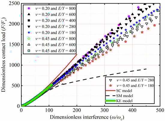
Figure 4.
F/Fc as a function of ω/ωc for different E and ν.
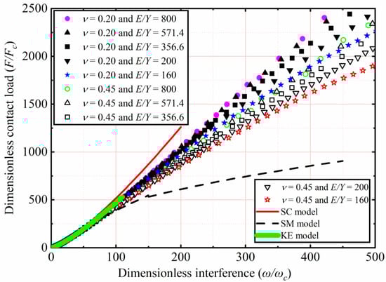
Figure 5.
F/Fc as a function of ω/ωc for different Y, ν, and E/Y > 133.3.
The effects of Y and ν shown in Table 3 on F/Fc as a function of ω/ωc are analyzed. Here E is a constant value equal to 200 GPa, while ν ranges from 0.2 to 0.45. With Y ranging from 1.25 to 0.25 GPa, corresponding to the E/Y ratios ranging from 160 to 800, which are all greater than 133.3, respectively. Here only the results of ν = 0.2 and 0.45 for E/Y = 160, 200, 356.6, 571.4, and 800 are selected and plotted in Figure 5. In the present interference domain, the SM model distinctly underestimates F/Fc. For 1< ω/ωc ≤ 110, the results indicate that the similarity with the KE model, F/Fc is independent of the Y and ν of the material. For 110 < ω/ωc ≤ 500, the present results show that the value of F/Fc decreases with an increasing Y. In addition, as ω/ωc increases for the material with a lower ν, the higher the F/Fc is for the fixed E/Y. In this work, the curve fitting of simulation data is carried out. For 133.3 < E/Y ≤ 800, 0.2 ≤ ν ≤ 0.45, and 1 < ω/ωc ≤ 500, the empirical expressions of F/Fc as a function of ω/ωc is presented in this paper as follows:
where m, n, and q are shown in Table 4.
Table 4.
Parameters in Equations (9) and (10).
When E/Y is less than 133.3, F/Fc as a function of ω/ωc for different Y and ν values is plotted in Figure 6. As shown in Table 3, E is 200 GPa, with ν = 0.2, 0.3, 0.4, and 0.45. With Y ranging from 2.52 to 1.5 GPa, corresponding to the E/Y ratio ranging from 79.4 to and 133.3, respectively.
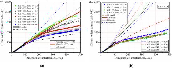
Figure 6.
F/Fc as a function of ω/ωc for different Y, ν, and E/Y ≤ 133.3: (a) E/Y = 133.3 and E/Y = 100; (b) E/Y = 79.4.
The results of ν = 0.2, 0.3, 0.4, and 0.45 for E/Y = 100 and 133.3 are selected and plotted in Figure 6a. F/Fc increases with an increasing ω/ωc. For 1 < ω/ωc ≤ 110, the present trend is like the KE model for all models. However, F/Fc is overestimated by the KE model for higher Y values and the interference near 110ωc. For 110 < ω/ωc ≤ 500, the present prediction results differ significantly from those of the JG model and MM model. Additionally, as ω/ωc increases, the lower the E/Y, the higher the deviation. At the value of ω/ωc equals 500, F/Fc deviation between present work and JG model is 15.82% when the E/Y ratio is 133.3 and 46.4% when the E/Y ratio is 100. In the present interference domain, MM model underestimates F/Fc.
The results of ν = 0.2, 0.3, 0.4, and 0.45 for E/Y = 79.4 are selected and plotted in Figure 6b. For 1 < ω/ωc ≤ 110, the present trend is similar to the KE model. For 110 < ω/ωc ≤ 500, the JG model overestimates F/Fc in the present interference domain. At the value of ω/ωc equals 500, F/Fc deviation between the present work and the JG model is 49.8% at the E/Y of 79.4. The obtained result is only similar to the SM model, which is valid only when the E/Y ratio is 79.4 and ν is 0.3. However, in present work, ν = 0.2, 0.3, 0.4, and 0.45 are further considered when the E/Y ratio is 79.4. It can be seen that F/Fc is affected by ν and that the lower the ν, the higher the F/Fc is with the increased ω/ωc. In this work, the curve fitting of simulation data is carried out. For 79.4 ≤ E/Y ≤ 133.3, 0.2 ≤ ν ≤ 0.45, and 1 < ω/ωc ≤ 500, the empirical expressions of F/Fc as a function of ω/ωc are presented in this paper as follows:
where m and n are shown in Table 5.
Table 5.
Parameters in Equation (11).
4.2. Contact Area
The effects of E and ν shown in Table 2 on A/Ac as a function of ω/ωc are analyzed. Here Y is a constant value equal to 0.25 GPa, with ν ranging from 0.2 to 0.45. With E ranging from 45 to 200 GPa, corresponding the E/Y ratios ranging from 180 to 800, respectively. Here only the results of ν = 0.2, 0.3, 0.4, and 0.45 for E/Y = 180 and 800 are selected and plotted in Figure 7. For 1 < ω/ωc ≤ 110, the results indicate the similarity with the KE model, and A/Ac is independent of E and ν. For 110 < ω/ωc ≤ 500, A/Ac increases with an increasing ω/ωc. In addition, the results show that E and ν have little effect on A/Ac. It is clear from Figure 7 that the SM model underestimates A/Ac as ω/ωc increases, especially for large interference. The reason of this discrepancy is that the SM model is valid only for an E/Y ratio of 79.4. The present result is slightly higher than the A/Ac predicted by the SC model with an increasing ω/ωc. The SC model analyzed the effect of tangential modulus on the elastic–plastic contact behavior, while the strain hardening effect is ignored in the present study. Compared with the predicted results of the SC model, it can be observed that tangential modulus has a great effect on the elastic–plastic contact behavior. In view of the shortcomings of present study, we will consider the effect of tangential modulus on hemispheric elastic–plastic contact behavior under large interference in future work.
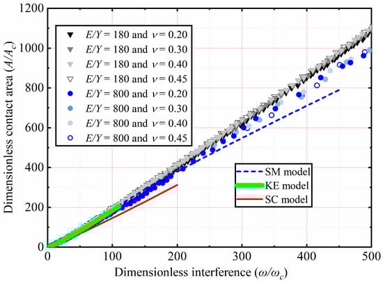
Figure 7.
A/Ac as a function of ω/ωc for different E and ν.
The effects of Y and ν, as shown in Table 3, on A/Ac as a function of ω/ωc are analyzed. Here E is 200 GPa, with ν ranging from 0.2 to 0.45. With Y ranging from 1.25 to 0.25 GPa, corresponding the E/Y ratios ranging from 160 to 800, respectively. Here only the results of ν = 0.2, 0.3, 0.4, and 0.45 for E/Y = 160 and 800 are selected and plotted in Figure 8. A/Ac increases with an increasing ω/ωc. For 1 < ω/ωc ≤ 110, the results indicate the similarity with the KE model, A/Ac is independent of Y and ν. For 110 < ω/ωc ≤ 500, Y and ν have little effect on A/Ac. Since the SM model is only suitable for E/Y = 79.4, A/Ac is underestimated in the present interference domain.
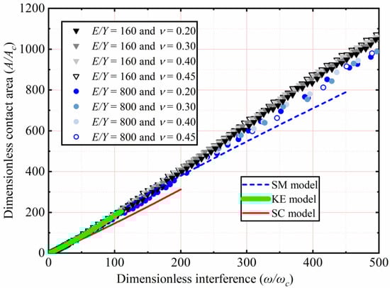
Figure 8.
A/Ac as a function of ω/ωc for different Y, ν, and E/Y > 133.3.
In Figure 7 and Figure 8, the effects of E, ν, and Y on A/Ac are comprehensively considered under an E/Y greater than 133.3. The results show that the E/Y ratio affects A/Ac. As the ω/ωc increases, the lower the E/Y, the higher the A/Ac is. ν has little effect on A/Ac. In this work, the curve fitting of simulation data is carried out. For 133.3 < E/Y ≤ 800, 0.2 ≤ ν ≤ 0.45, and 1 < ω/ωc ≤ 500, the empirical expressions of A/Ac as a function of ω/ωc is presented in this paper as follows:
where m and n are shown in Table 6.
Table 6.
Parameters in Equation (12).
When the ratio of E/Y is less than 133.3, A/Ac as a function of ω/ωc for different Y and ν values is plotted in Figure 9. Here E is a constant value equal to 200 GPa, with ν ranging from 0.2 to 0.45. With Y being 2.52, 2, and 1.5 GPa, corresponding the E/Y ratio is 79.4, 100, and 133.3, respectively. ω/ωc ranges from 1 to 500. At small interferences, the dependence of A/Ac on Y and ν is weak, which is similar to the prediction of KE model. However, with an increasing ω/ωc, the influence of Y on A/Ac is strong. It is clear from Figure 9 that the present A/Ac is consistent with that predicted by the SM model for E/Y = 79.4. However, A/Ac is underestimated by the SM model when the E/Y is greater than 79.4. It can also be seen that in the present ω/ωc domain, the JG model overestimates A/Ac. At a ω/ωc value of 500, A/Ac deviation between the present work and JG model is 70.73% when E/Y is 133.3 and 25.1% when E/Y is 79.4. When E/Y is greater than 133.3, the error of the JG model is slightly less than that of other models compared with the present predicted results. To overcome the drawbacks of previous models, the curve fitting of the simulation data is carried out in this work. For 79.4 ≤ E/Y ≤ 133.3, 0.2 ≤ ν ≤ 0.45, and 1 < ω/ωc ≤ 500, the empirical formulas for predicting the contact area are presented in this paper as follows:
where m and n are shown in Table 7.
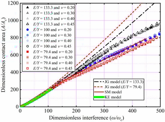
Figure 9.
A/Ac as a function of ω/ωc for different Y, ν and E/Y ≤ 133.3.
Table 7.
Parameters in Equation (13).
4.3. Contact Pressure
The effects of E and ν shown in Table 2 on p/Y as a function of ω/ωc are analyzed. Here, Y is a constant value equal to 0.25 GPa, with ν ranging from 0.2 to 0.45. With E ranging from 45 to 200 GPa, corresponding the E/Y ratios ranging from 180 to 800, respectively. Here, only the results of ν = 0.2 and 0.45 for E/Y = 180, 400, and 800 are selected and plotted in Figure 10. The KE model considered that p/Y reaching the peak could be marked the contact state transition from the elastic–plastic to the fully plastic and that the corresponding ω/ωc is a constant value equal to 110. Through this, the elastic–plastic range (1 ≤ ω/ωc ≤ 110) is proposed by the KE model. However, this tendency is not observed in the present work. It is obvious that ω/ωc corresponding to the peak value of p/Y is not fixed but is dependent on E and ν in all cases. It is clear from Figure 10 that the peak value of p/Y also increases with an increasing E. Additionally, the value of ν increases, the peak value of p/Y also increases under constant E/Y. By comparison, the effects of ν are less than that of E on the peak value of p/Y.
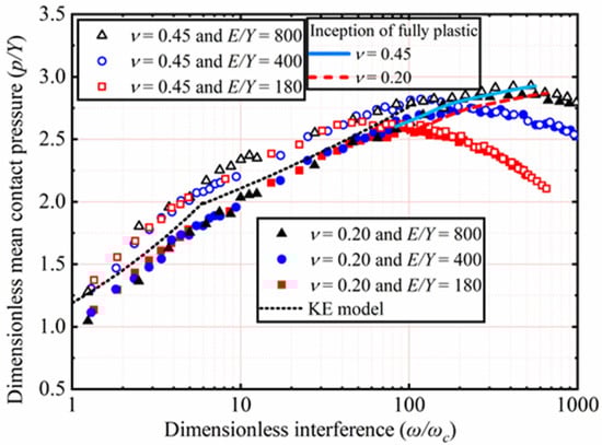
Figure 10.
p/Y as a function of ω/ωc for different E and ν.
After p/Y reaches its peak value, namely the fully plastic range, it is no longer affected by ν, as shown in Figure 10. In the fully plastic range, p/Y decreases with an increasing ω/ωc. Moreover, the results also show that this trend is more evident with the lower E value, which is the same as the observational results of the SC model. Interestingly, the results obtained show that before p/Y reaches its peak in all cases, namely the elastic–plastic range, the higher ν, the higher p/Y is.
The effects of Y and ν, as shown in Table 3, on p/Y as a function of ω/ωc are analyzed. Here E is a constant value equal to 200 GPa, with ν ranging from 0.2 to 0.45. With Y ranging from 2.52 to 0.25 GPa, corresponding the E/Y ratios ranging from 79.4 to 800, respectively. Here only the results of ν = 0.2 and 0.45 for E/Y = 79.4, 133.3, 200, 356.6, and 800 are selected and plotted in Figure 11. In the elastic–plastic range, p/Y increases with an increasing ω/ωc. Additionally, the higher ν, the higher p/Y is. p/Y decreases with an increasing ω/ωc in the plastic range. The results show that this trend is more evident with the higher Y value. Moreover, ν has no longer has an effect on p/Y in the fully plastic range.
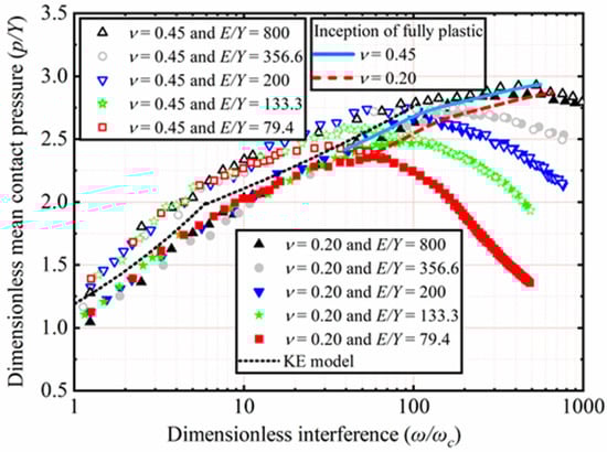
Figure 11.
p/Y as a function of ω/ωc for different Y and ν.
The present work has observed that in all cases, ω/ωc corresponding to the peak value of p/Y is not limited to a specific value of 110 predicted by the KE model but depends on Y and ν. It is clear from Figure 11 that the peak value of p/Y also increases when Y decreases. Moreover, as ν increases, the peak value of p/Y also increases under constant E/Y. By comparison, the effects of ν are less than Y for the peak value of p/Y.
4.4. Elastic–Plastic Range
Figure 12 shows the end of the elastic–plastic deformation () as a function of E/Y. In addition, comparisons with the KE model are also depicted. The KE model suggested that p/Y reaches the peak and marks the transition from the elastic–plastic to the fully plastic deformation regime, and the corresponding is the constant value equal to 110. The method of using the maximum value of p/Y to find the end of the elastic–plastic deformation regime can also be found in Kogut et al. [31,36]. The present results show that the value of increases with an increasing of E/Y and is not the constant value equal to 110 predicted by the KE model. For all of E/Y, the higher the value of ν, the lower value of . The present results also show that the value of . is about 110 at E/Y = 200, which is consistent with the predicted result of the KE model. Moreover, when the E/Y is less than 200, the KE model overestimates the value of . Therefore, to estimate the value of and predict the end of the elastic–plastic range, the empirical formula is proposed in this work as follows:
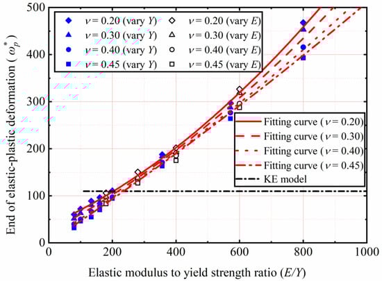
Figure 12.
as a function of E/Y.
As mentioned above, the corresponding ωc at the inception of the elastic–plastic deformation regime can be determined by using Equation (4). Additionally, the corresponding at the end of elastic–plastic deformation regime can be determined by using Equation (14). Furthermore, to estimate the contact parameters of the elastic–plastic range, the empirical formula is proposed in this work as follows:
where m, n, q, and t are shown in Table 8.
Table 8.
Parameters in Equations (15) and (16).
In order to more conveniently use the elastic–plastic constitutive relation presented in this paper, a flowchart for predicting the contact parameters in the purely elastic, elastic–plastic, and fully plastic ranges is shown in Figure 13. First, for the purely elastic contact stage, the contact parameters are calculated according to Equations (5) and (6). Secondly, for the elastic–plastic range, the contact parameters are calculated according to Equations (15) and (16). Additionally, and lastly, for large deformations, it includes the elastic–plastic and fully plastic range. If 0.2 ≤ ν ≤ 0.45 and 79.4 ≤ E/Y ≤ 133.3, the contact parameters are calculated according to Equations (11) and (13), otherwise according to the Equations (9)–(12).
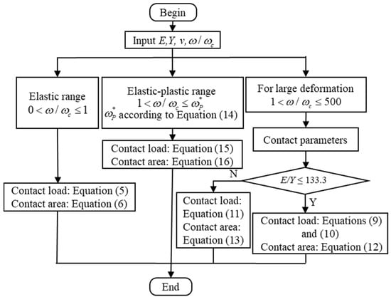
Figure 13.
Flowchart for predicting the contact parameters.
4.5. Comparison with Experimental Results
To verify the rationality of the present model, the present predicted contact load and area are compared with Ovcharenko et al. [28] and Jamari and Schipper [27] experimental data.
Jamari and Schipper [27] experimentally measured the relationship between the contact parameters of the copper sphere and the SiC ceramic flat. In their experiment, the material parameters of the copper sphere are E = 120 GPa, R = 1.5 mm, ν = 0.35, H = 1.2 GPa, and E/Y = 280, respectively. As their material parameter is E/Y = 280, Jamari and Schipper’s experimental results were compared with the present prediction formula of the Equation (12) and the results are shown in Figure 14. The present prediction results are in good agreement with the experimental ones, which verifies the accuracy of the present work.
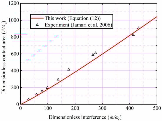
Figure 14.
Comparison with experimental result for the copper [27].
Ovcharenko et al. [28] experimentally measured the relationship between the contact load and the area of the stainless-steel and copper spheres in contact with the Sapphire flat. As shown in the Figure 15. the present predicted results are compared with the Ovcharenko et al. experimental results for the copper and stainless-steel. Compared with the Jamari and Schipper experimental study, Ovcharenko et al. only analyzed the contact area under small loads through their experiments. It is clear from Figure 15 that the present model is in good agreement with the experimental results and the error is less than 10%, indicating that the proposed model has a high accuracy. This discrepancy may be due to the fact that the SiC ceramic flat in the experiment is not as rigid as assumed in the theoretical model, leading to some error between the experimental and theoretical results.
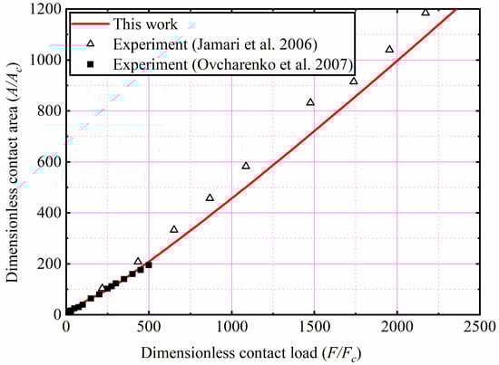
Figure 15.
Comparison with experimental results for the stainless-steel and copper [27,28].
5. Conclusions
A flattening contact behavior of an elastic–perfectly plastic hemisphere against a rigid flat was researched by using FEM. The present analysis addresses the effects of Poisson’s ratio, elastic modulus, and yield strength on the contact behavior. The main conclusions can be drawn as follows:
- (1)
- The present study considers a large range of dimensionless interference from 1 to 500. A new elastic–plastic constitutive model is proposed to predict the contact area and load based on the curve fitting the finite analyses results. Compared with previous models and experiments, the rationality of the present model is verified.
- (2)
- p/Y is mainly affected by the ν in the elastic–plastic range, and the higher the ν, the higher p/Y. However, this influence disappears in the fully plastic range. The maximum of p/Y is not a constant value for the different E, Y, and ν. The higher E/Y, the higher the maximum of p/Y is. Moreover, the higher ν, the higher the maximum value of p/Y is when E/Y is constant. However, the effects of ν are less than that of E and Y for the maximum value of p/Y. In the plastic range, p/Y decreases with increasing interference. Additionally, the lower E/Y, the more noticeable this trend is.
- (3)
- The boundaries between the elastic, elastic–plastic, and fully plastic deformation regimes are determined according to the interference, maximum mean contact pressure, Poisson’s ratio, and the elastic modulus to yield strength ratio. When the interference is small, the contact state is purely elastic, and the contact parameters can be calculated according to the Hertz formula. When the interference increases, the contact state changes from the purely elastic to the elastic–plastic. The present work shows that the JG model can more reasonably determine the inception of elastic–plastic deformation regime. The end of the elastic–plastic deformation regime is defined according to the interference corresponding to the maximum contact pressure. New dimensionless constitutive relationships are proposed to predict the contact parameters in the elastic–plastic range.
Author Contributions
Conceptualization, J.C. and L.Z.; methodology, J.C.; validation, J.C. and W.Z.; formal analysis, J.C. and W.Z.; investigation, J.C. and W.Z.; resources, J.C., W.Z. and D.L.; data curation, J.C., L.Z. and W.Z.; writing original draft preparation, J.C. and W.Z.; writing review and editing, L.Z. supervision, L.Z., W.Z. and C.W.; project administration, C.W.; funding acquisition, D.L. All authors have read and agreed to the published version of the manuscript.
Funding
This research was funded by the National Natural Science Foundation of China, grant number 52005381.
Institutional Review Board Statement
Not applicable.
Informed Consent Statement
Not applicable.
Data Availability Statement
Not applicable.
Acknowledgments
The authors are grateful for the comments and help of reviewers and editors.
Conflicts of Interest
The authors declare no conflict of interest.
Nomenclature
| a | Contact radius |
| p | Mean contact pressure |
| p0 | Maximum Hertzian pressure |
| A | Contact area |
| C | Critical yield stress coefficient |
| E | Equivalent elastic modulus |
| F | Contact load |
| Critical interference value at the inception fully plastic | |
| R | The radius of asperity |
| Y | Yield strength |
| ν | Poisson’s ratio |
| ω | Normal interference of asperity |
| Scripts | |
| 1 | The value of asperity |
| 2 | The value of rigid flat |
| c | Critical values at yielding inception |
| p | Critical values at the end of the elastic–plastic range |
| * | Dimensionless |
| e | Elastic range |
| ep | Elastic–plastic range |
References
- Wang, H.; Yin, X.; Hao, H.; Chen, W.; Yu, B. The correlation of theoretical contact models for normal elastic-plastic impacts. Int. J. Solids Struct. 2020, 182, 15–33. [Google Scholar] [CrossRef]
- Edmans, B.D.; Sinka, I.C. Unloading of elastoplastic spheres from large deformations. Powder Technol. 2020, 374, 618–631. [Google Scholar] [CrossRef]
- Johnson, K.L. Contact Mechanics; Cambridge University: Cambridge, UK, 1985. [Google Scholar]
- Ghaednia, H.; Wang, X.; Saha, S.; Xu, Y.; Sharma, A.; Jackson, R.L. A review of elastic-plastic contact mechanics. Appl. Mech. Rev. 2017, 69, 30. [Google Scholar] [CrossRef]
- Weng, P.; Yin, X.; Hu, W.; Yuan, H.; Chen, C.; Ding, H.; Yu, B.; Xie, W.; Jiang, L.; Wang, H. Piecewise linear deformation characteristics and a contact model for elastic-plastic indentation considering indenter elasticity. Tribol. Int. 2021, 162, 107–114. [Google Scholar] [CrossRef]
- Li, B.; Li, P.; Zhou, R.; Feng, X.; Zhou, K. Contact mechanics in tribological and contact damage-related problems: A review. Tribol. Int. 2022, 171, 107534. [Google Scholar] [CrossRef]
- Heath, C.E.; Feng, S.; Day, J.P.; Graham, A.L.; Ingber, M.S. Near-contact interactions between a sphere and a plane. Phys. Rev. E 2008, 77, 1110–1114. [Google Scholar] [CrossRef]
- Li, L.; Etsion, I.; Talke, F.E. Elastic–plastic spherical contact modeling including roughness effects. Tribol. Lett. 2010, 40, 357–363. [Google Scholar] [CrossRef]
- Updike, D.P.; Kalnins, A. Contact pressure between an elastic spherical shell and a rigid plate. J. Appl. Mech. 1972, 39, 1110–1114. [Google Scholar] [CrossRef]
- Kutzner, I.; Trepczynski, A.; Heller, M.O.; Bergmann, G. Knee adduction moment and medial contact force—facts about the correlation during gait. J. Biomech. 2012, 45, S381. [Google Scholar] [CrossRef]
- Chu, N.R.; Jackson, R.L.; Wang, X.; Gangopadhyay, A.; Ghaednia, H. Evaluating elastic-plastic wavy and spherical asperity based statistical and multi-scale rough surface contact models with deterministic results. Materials 2021, 14, 3864. [Google Scholar] [CrossRef]
- Gao, Z.; Fu, W.; Wang, W.; Kang, W.; Liu, Y. The study of anisotropic rough surfaces contact considering lateral contact and interaction between asperities. Tribol. Int. 2018, 126, 270–282. [Google Scholar] [CrossRef]
- Yuan, Y.; Cheng, Y.; Liu, K.; Gan, L. A revised Majumdar and Bushan model of elastoplastic contact between rough surfaces. Appl. Surf. Sci. 2017, 425, 1138–1157. [Google Scholar] [CrossRef]
- Ren, W.; Zhang, C.; Sun, X. Electrical contact resistance of contact bodies with cambered surface. IEEE Access 2020, 8, 93857–93867. [Google Scholar] [CrossRef]
- Angadi, S.V.; Jackson, R.L.; Pujar, V.; Tushar, M.R. A comprehensive review of the finite element modeling of electrical connectors including their contacts. IEEE T Comp. Pack. Man. 2020, 10, 836–844. [Google Scholar] [CrossRef]
- Jackson, R.L.; Ghaednia, H.; Elkady, Y.A.; Bhavnani, S.H.; Knight, R.W. A closed-form multiscale thermal contact resistance model. ieee transactions on components. IEEE T Comp. Pack. Man. 2012, 2, 1158–1171. [Google Scholar]
- Ghaednia, H.; Jackson, R.L.; Gao, J. A Third Body Contact Model for Particle Contaminated Electrical Contacts; IEEE: Piscataway, NJ, USA, 2014. [Google Scholar]
- Lontin, K.; Khan, M. Interdependence of friction, wear, and noise: A review. Friction 2021, 9, 1319–1345. [Google Scholar] [CrossRef]
- Wang, H.; Zhou, C.; Hu, B.; Li, Y. An adhesive wear model of rough gear surface considering modified load distribution factor. Proc. Inst. Mech. Eng. Part J. Eng. Tribol. 2022, 1, 135065012210748. [Google Scholar] [CrossRef]
- Ghaednia, H.; Jackson, R.L. The Effect of nanoparticles on the real area of contact, friction, and wear. J. Tribol. 2013, 135, 041603. [Google Scholar] [CrossRef]
- Gholami, R.; Ghaemi, K.H.; Silani, M.; Akbarzadeh, S. Experimental and numerical investigation of friction coefficient and wear volume in the mixed-film lubrication regime with ZNO nano-particle. J. Appl. Fluid Mech. 2020, 13, 993–1001. [Google Scholar] [CrossRef]
- Greenwood, J.A.; Williamson, J.B.P. Contact of nominally fat surfaces. Proc. R. Soc. Lond. A 1966, 295, 300–319. [Google Scholar]
- Hertz, H. Ueber die Berührung Fester Elastischer Körper. J. Reine. Angew. Math. 1881, 92, 156–171. [Google Scholar]
- Lin, L.P.; Lin, J.F. An elastoplastic microasperity contact model for metallic materials. J. Tribol. 2005, 127, 666–672. [Google Scholar]
- Chang, W.R.; Etsion, I.; Bogy, D.B. An elastic-plastic model for the contact of rough surfaces. J. Tribol. 1987, 109, 257–263. [Google Scholar] [CrossRef]
- Chang, W.R.; Etsion, I.; Bogy, D.B. Adhesion model for metallic rough surfaces. J. Tribol. 1988, 110, 50–56. [Google Scholar] [CrossRef]
- Jamari, J.; Schipper, D.J. Experimental investigation of fully plastic contact of a sphere against a hard flat. J. Tribol. 2006, 128, 230–235. [Google Scholar] [CrossRef][Green Version]
- Ovcharenko, A.; Halperin, G.; Verberne, G.; Etsion, I. In situ investigation of the contact area in elastic–plastic spherical contact during loading-unloading. Tribol. Lett. 2007, 25, 153–1607. [Google Scholar] [CrossRef]
- Sahoo, P.; Chatterjee, B. Effect of strain hardening on elastic-plastic contact of a deformable sphere against a rigid flat under full stick contact condition. Adv. Tribol. 2012, 2012, 1–8. [Google Scholar]
- Sahoo, P.; Chatterjee, B. Finite element based unloading of an elastic plastic spherical stick contact for varying tangent modulus and hardening rule. Int. J. Surf. Eng. Interdiscip. Mater. Sci. 2013, 1, 13–32. [Google Scholar]
- Kogut, L.; Etsion, I. Elastic-plastic contact analysis of a sphere and a rigid flat. J. Appl. Mech 2002, 69, 657–662. [Google Scholar] [CrossRef]
- Green, I. Poisson ratio effects and critical values in spherical and cylindrical hertzian contacts. Int. J. Appl. Mech. Eng. 2004, 10, 451–462. [Google Scholar]
- Jackson, R.L.; Green, I. A finite element study of elasto-plastic hemispherical contact against a rigid flat. J. Tribol. 2005, 127, 343–354. [Google Scholar] [CrossRef]
- Tabor, D. The Hardness of Metals; Clarendon Press: Oxford, UK, 1951. [Google Scholar]
- Quicksall, J.J.; Jackson, R.L.; Green, I. Elasto-plastic hemispherical contact models for various mechanical properties. Proc. Inst. Mech. Eng. Part J J. Eng. Tribol. 2004, 218, 313–322. [Google Scholar] [CrossRef]
- Kogut, L.; Komvopoulos, K. Analysis of the spherical indentation cycle for elastic-perfectly plastic solids. J. Mater. Res. 2004, 19, 3641–3653. [Google Scholar] [CrossRef]
- Brizmer, V.; Kligerman, Y.; Etsion, I. The effect of contact conditions and material properties on the elasticity terminus of a spherical contact. Int. J. Solids Struct. 2006, 43, 5736–5749. [Google Scholar] [CrossRef]
- Shankar, S.; Mayuram, M.M. A finite element based study on the elastic-plastic transition behavior in a hemisphere in contact with a rigid flat. J. Tribol. 2008, 130, 6. [Google Scholar] [CrossRef]
- Shankar, S.; Mayuram, M.M. Effect of strain hardening in elastic-plastic transition behavior in a hemisphere in contact with a rigid flat. Int. J. Solids Struct. 2008, 45, 3009–3020. [Google Scholar] [CrossRef]
- Malayalamurthi, R.; Marappan, R. Elastic-plastic contact behavior of a sphere loaded against a rigid flat, mech. Adv. Mater. Struc. 2008, 15, 364–370. [Google Scholar] [CrossRef]
- Sahoo, P.; Chatterjee, B. A finite element study of elastic-plastic hemispherical contact behavior against a rigid flat under varying modulus of elasticity and sphere radius. Engineering 2010, 2, 205–211. [Google Scholar] [CrossRef]
- Sahoo, P.; Chatterjee, B.; Adhikary, D. Finite element based elastic-plastic contact behavior of a sphere against a rigid flat—Effect of strain hardening. Int. J. Eng. Technol. 2010, 2, 1–6. [Google Scholar]
- Megalingam, A.; Mayuram, M.M. A comprehensive elastic-plastic single-asperity contact model. Tribol. T. 2014, 57, 324–335. [Google Scholar] [CrossRef]
- Megalingam, A.; Hanumanth Ramji, K.S. A complete elastic-plastic spherical asperity contact model with the effect of isotropic strain hardening. Proc. Inst. Mech. Eng. Part J J. Eng. Tribol. 2021, 235, 820–829. [Google Scholar] [CrossRef]
- Ghaednia, H.; Mifflin, G.; Lunia, P.; O’Neill, E.O.; Brake, M.R.W. Strain hardening from elastic-perfectly plastic to perfectly elastic indentation single asperity contact. Front. Mech. Eng. 2020, 6, 60. [Google Scholar] [CrossRef]
- Ghaednia, H.; Brake, M.R.W.; Berryhill, M.; Jackson, R.L. Strain hardening from elastic-perfectly plastic to perfectly elastic flattening single asperity contact. J. Tribol. 2019, 141, 11. [Google Scholar] [CrossRef]
- Ghaednia, H.; Pope, S.A.; Jackson, R.L.; Marghitu, D.B. A comprehensive study of the elasto-plastic contact of a sphere and a flat. Tribol. Int. 2016, 93, 78–90. [Google Scholar] [CrossRef]
- Ashby, M.F.; Jones, D.R.H. Engineering Materials 1: An Introduction to Properties, Applications, and Design, 4th ed.; Butter-worth-Heinemann: Amsterdam, The Netherlands, 2012; p. 472. [Google Scholar]
Publisher’s Note: MDPI stays neutral with regard to jurisdictional claims in published maps and institutional affiliations. |
© 2022 by the authors. Licensee MDPI, Basel, Switzerland. This article is an open access article distributed under the terms and conditions of the Creative Commons Attribution (CC BY) license (https://creativecommons.org/licenses/by/4.0/).