
Effects of Multiple Financial News Shocks on Tourism Demand Volatility Modelling and Forecasting

 ,
,  and
and
Abstract
:1. Introduction
2. Literature Review
2.1. News Shocks in Tourism Demand Volatility
2.2. Symmetric and Asymmetric Effects on Tourism Demand Volatility
2.3. Studies of Symmetric and Asymmetric Effects across on the News Shocks for Tourism Forecasting
2.4. The Economics Index in This Research
2.5. News Shocks for Malaysia
3. Model Description
3.1. Volatility Models with Financial News Shocks
3.2. Evaluation Criterion
4. Data Description
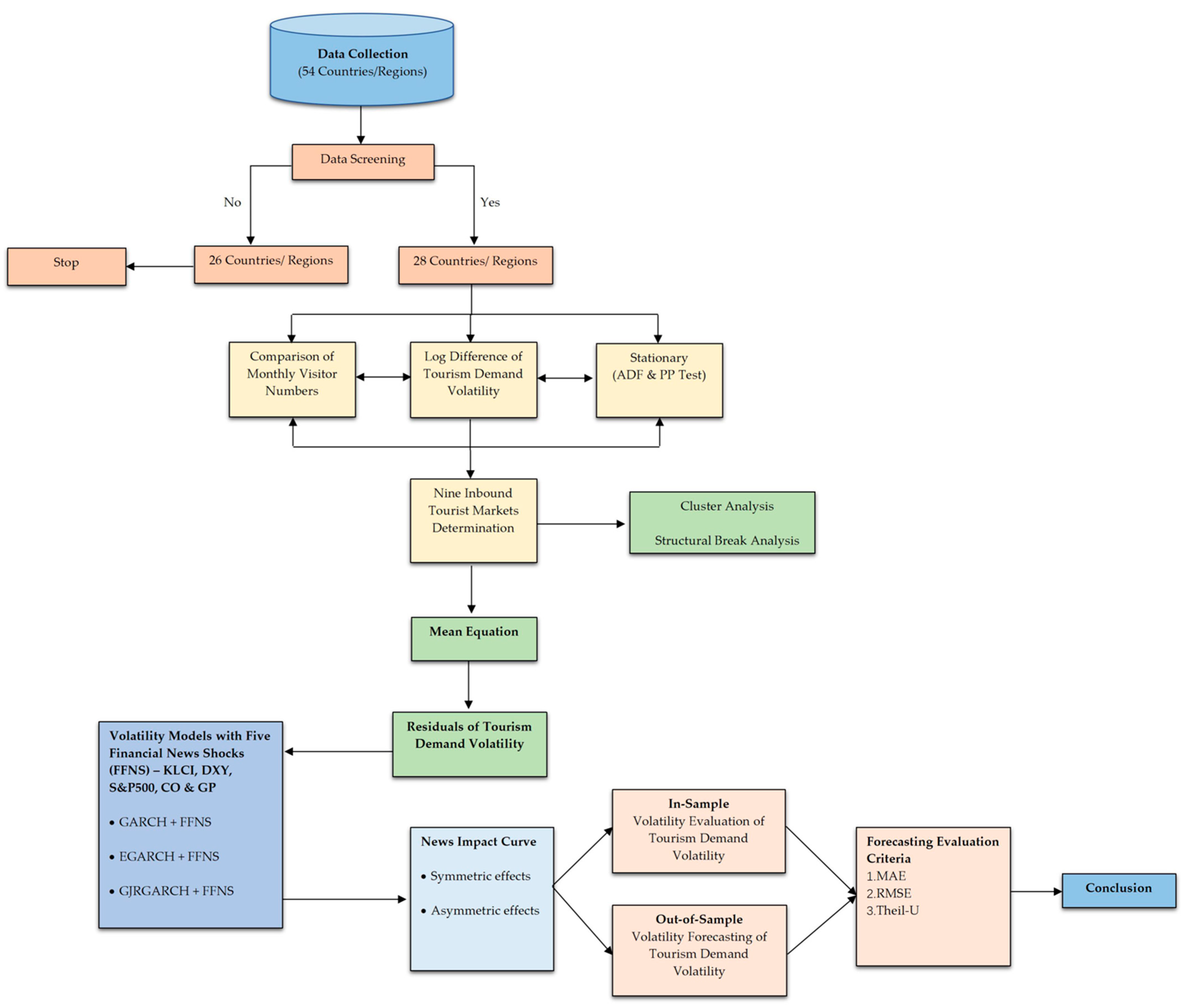
5. Research Process
6. Empirical Results
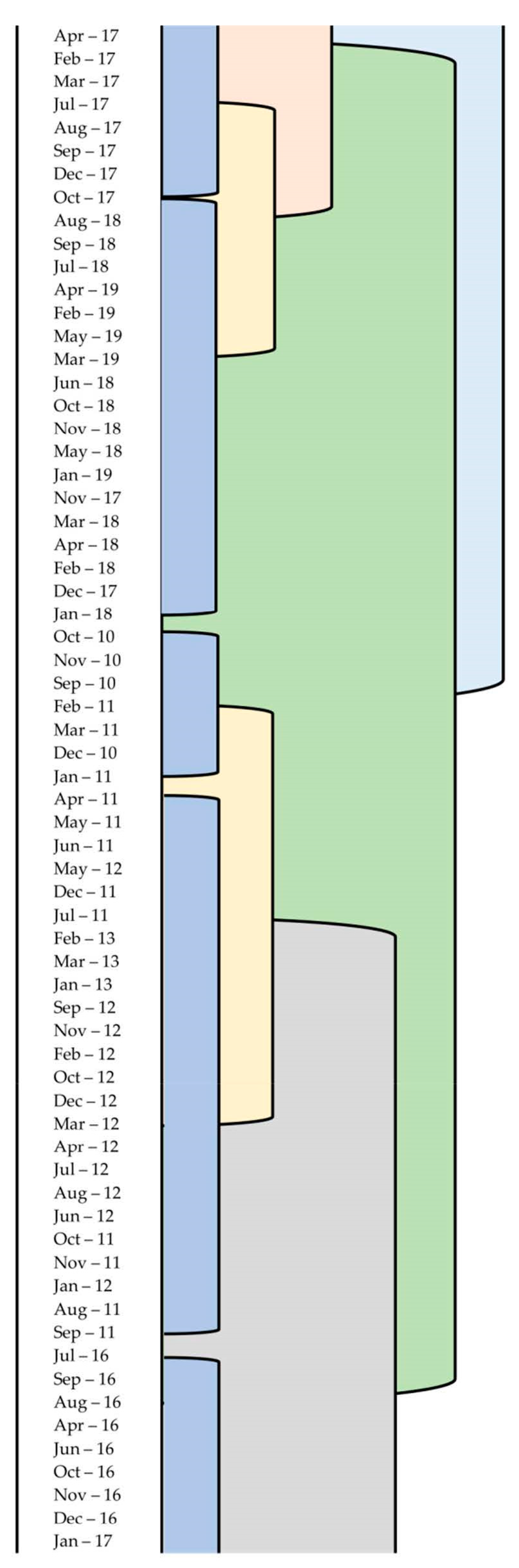
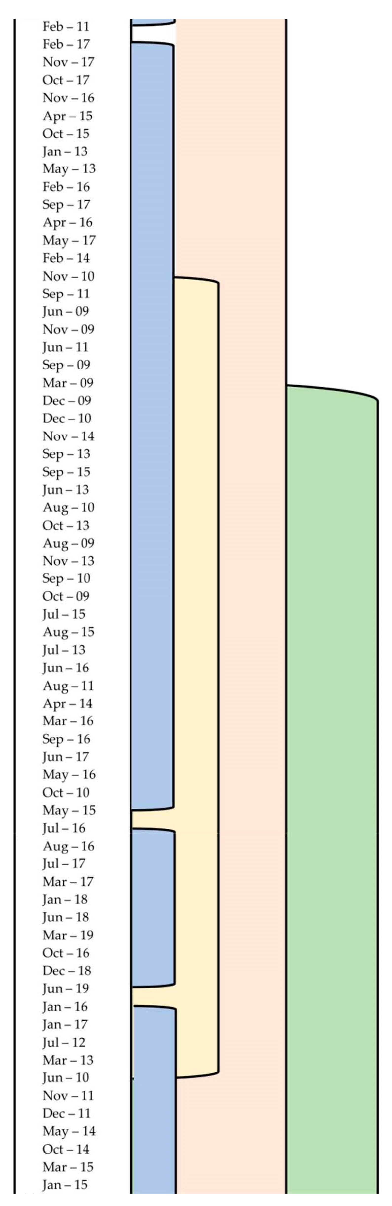
6.1. Cluster Analysis
6.2. Structural Break Analysis
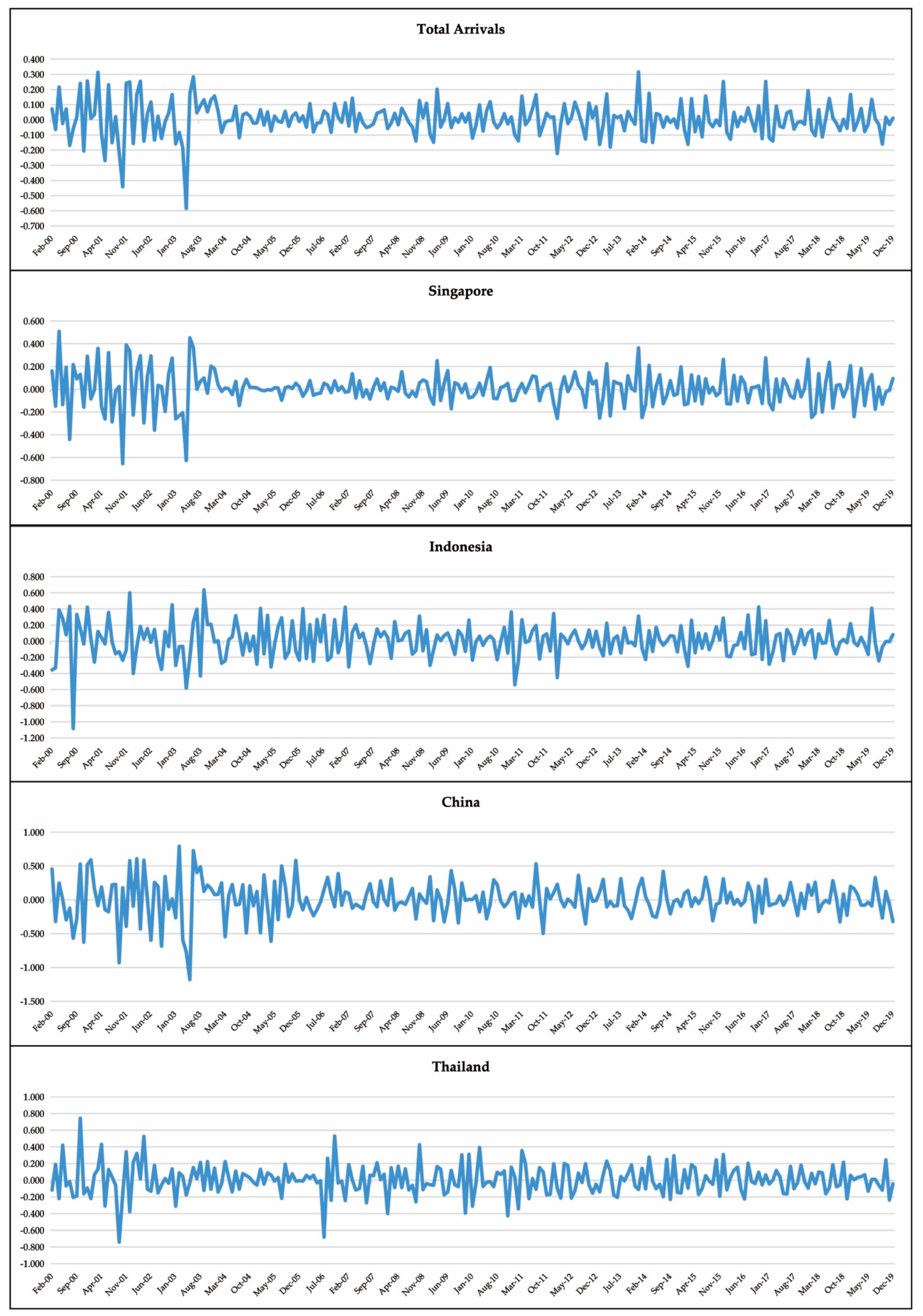
6.3. Unit Root Test
6.4. Estimation and Diagnostic Tests of Methods for Modelling
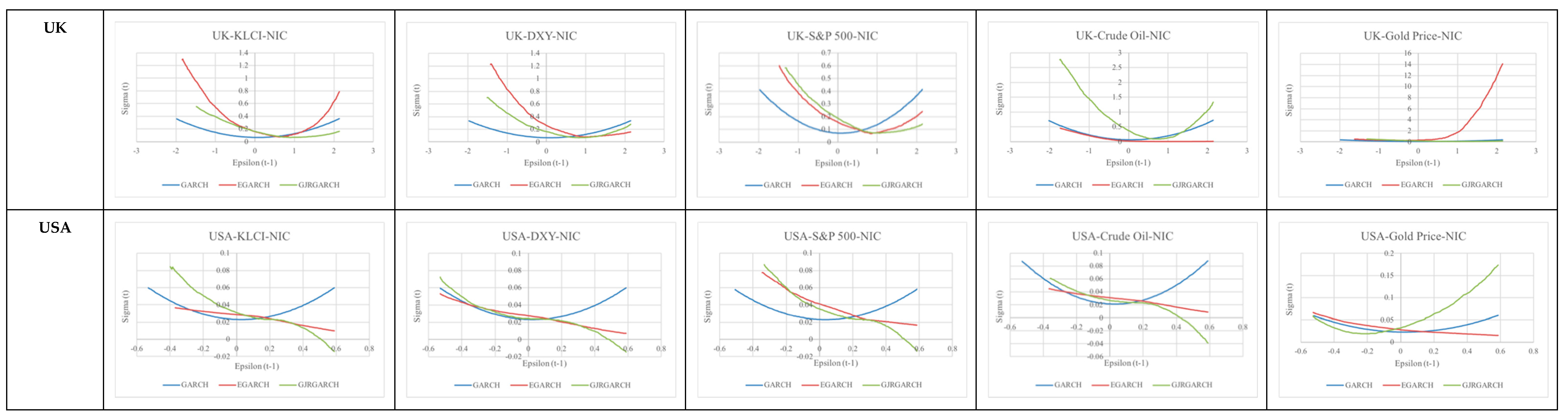
6.5. Estimation of News Impact Curve
6.6. In-Sample Prediction Performance
6.7. Post-Sample Forecasting Performance
7. Conclusions
Author Contributions
Funding
Institutional Review Board Statement
Informed Consent Statement
Data Availability Statement
Acknowledgments
Conflicts of Interest
References
- Agiomirgianakis, George, Dimitrios Serenis, and Nicholas Tsounis. 2015. Effects of exchange rate volatility on tourist flows into Iceland. Procedia Economics and Finance 24: 25–34. [Google Scholar] [CrossRef] [Green Version]
- Akar, Cüneyt. 2012. Modeling Turkish tourism demand and the exchange rate: The bivariate GARCH approach. European Journal of Economics, Finance and Administrative Science 50. Available online: https://ssrn.com/abstract=2914133 (accessed on 18 June 2022).
- Alleyne, Laron Delano, Onoh-Obasi Okey, and Winston Moore. 2020. The volatility of tourism demand and real effective exchange rates: A disaggregated analysis. Tourism Review 76: 489–502. [Google Scholar] [CrossRef]
- Bai, Jushan, and Pierre Perron. 1998. Estimating and testing linear models with multiple structural changes. Econometrica 66: 47–78. [Google Scholar] [CrossRef]
- Balli, Hatice Ozer, Wai Hong Kan Tsui, and Faruk Balli. 2019. Modelling the volatility of international visitor arrivals to New Zealand. Journal of Air Transport Management 75: 204–14. [Google Scholar] [CrossRef]
- Bartolomé, Ana, Michael McAleer, Vicente Ramos, and Javier Rey-Maquieira. 2009. Modelling air passenger arrivals in the Balearic and Canary Islands, Spain. Tourism Economics 15: 481–500. [Google Scholar] [CrossRef]
- Becken, Susanne, and James Lennox. 2012. Implications of a long-term increase in oil prices for tourism. Tourism Management 33: 133–42. [Google Scholar] [CrossRef] [Green Version]
- Berndt, Ernst R., Bronwyn H. Hall, Robert E. Hall, and Jerry A. Hausman. 1974. Estimation and inference in nonlinear structural models. Annals of Economic and Social Measurement 3: 653–65. [Google Scholar]
- Bhattarai, Keshav, Dennis Conway, and Nanda Shrestha. 2005. Tourism, terrorism and turmoil in Nepal. Annals of Tourism Research 32: 669–88. [Google Scholar] [CrossRef]
- Bollerslev, Tim. 1986. Generalized autoregressive conditional heteroskedasticity. Journal of econometrics 31: 307–27. [Google Scholar] [CrossRef] [Green Version]
- Bronner, Fred, and Robert de Hoog. 2017. Tourist demand reactions: Symmetric or asymmetric across the business cycle? Journal of Travel Research 56: 839–53. [Google Scholar] [CrossRef] [PubMed]
- Byrne, Joseph P., and E. Philip Davis. 2005. The impact of short-and long-run exchange rate uncertainty on investment: A panel study of industrial countries. Oxford Bulletin of Economics and Statistics 67: 307–29. [Google Scholar] [CrossRef]
- Çelik, Gülşah Gençer. 2020. Volatility Modelling for Tourism Sector Stocks in Borsa Istanbul. International Journal of Economics and Financial Issues 10: 158. [Google Scholar] [CrossRef]
- Chan, Felix, Christine Lim, and Michael McAleer. 2005. Modelling multivariate international tourism demand and volatility. Tourism Management 26: 459–71. [Google Scholar] [CrossRef]
- Chang, Chia-Lin, and Michael McAleer. 2009. Daily Tourist Arrivals, Exchange Rates and Voatility for Korea and Taiwan. Korean Economic Review 25: 241–67. [Google Scholar]
- Chang, Chia-Lin, and Michael McAleer. 2012. Aggregation, heterogeneous autoregression and volatility of daily international tourist arrivals and exchange rates. The Japanese Economic Review 63: 397–419. [Google Scholar] [CrossRef] [Green Version]
- Chatziantoniou, Ioannis, George Filis, Bruno Eeckels, and Alexandros Apostolakis. 2013. Oil prices, tourism income and economic growth: A structural VAR approach for European Mediterranean countries. Tourism Management 36: 331–41. [Google Scholar] [CrossRef] [Green Version]
- Chen, Ching-Fu, and Song Zan Chiou-Wei. 2009. Tourism expansion, tourism uncertainty and economic growth: New evidence from Taiwan and Korea. Tourism Management 30: 812–18. [Google Scholar] [CrossRef]
- Chi, Junwook. 2015. Dynamic impacts of income and the exchange rate on US tourism, 1960–2011. Tourism Economics 21: 1047–60. [Google Scholar] [CrossRef]
- Chikobvu, Delson, and Tendai Makoni. 2019. Statistical modelling of Zimbabwe’s international tourist arrivals using both symmetric and asymmetric volatility models. Journal of Economic and Financial Sciences 12: a426. [Google Scholar] [CrossRef]
- Chong, Choo Wei, Muhammad Idrees Ahmad, and Mat Yusoff Abdullah. 1999. Performance of GARCH models in forecasting stock market volatility. Journal of Forecasting 18: 333–43. [Google Scholar] [CrossRef]
- Coshall, John T. 2009. Combining volatility and smoothing forecasts of UK demand for international tourism. Tourism Management 30: 495–511. [Google Scholar] [CrossRef]
- Coshall, John T., and Richard Charlesworth. 2011. A management orientated approach to combination forecasting of tourism demand. Tourism Management 32: 759–69. [Google Scholar] [CrossRef]
- Croes, Robertico R., and Manuel Vanegas Sr. 2005. An econometric study of tourist arrivals in Aruba and its implications. Tourism Management 26: 879–90. [Google Scholar] [CrossRef]
- Cró, Susana, and António Miguel Martins. 2017. Structural breaks in international tourism demand: Are they caused by crises or disasters? Tourism Management 63: 3–9. [Google Scholar] [CrossRef]
- Demir, Cengiz. 2004. How do monetary operations impact tourism demand? The case of Turkey. International Journal of Tourism Research 6: 113–17. [Google Scholar] [CrossRef]
- Demirel, Baki, Barış Alparslan, Emre Güneşer Bozdağ, and Alp Gökhun İncİ. 2013. The Impact Of Exchange Rate Volatılıty On Tourısm Sector: A Case Study, Turkey. Niğde Üniversitesi İktisadi ve İdari Bilimler Fakültesi Dergisi 6: 117–26. [Google Scholar]
- Dutta, Anupam, Tapas Mishra, Gazi Salah Uddin, and Yang Yang. 2021. Brexit uncertainty and volatility persistence in tourism demand. Current Issues in Tourism 24: 2225–32. [Google Scholar] [CrossRef]
- Emili, Silvia, Paolo Figini, and Andrea Guizzardi. 2020. Modelling international monthly tourism demand at the micro destination level with climate indicators and web-traffic data. Tourism Economics 26: 1129–51. [Google Scholar] [CrossRef]
- Engle, Robert F. 1982. Autoregressive conditional heteroscedasticity with estimates of the variance of United Kingdom inflation. Econometrica: Journal of the Econometric Society 50: 987–1007. [Google Scholar] [CrossRef]
- Engle, Robert F., and Clive W. J. Granger. 1987. Co-integration and error correction: Representation, estimation, and testing. Econometrica: Journal of the Econometric Society 55: 251–76. [Google Scholar] [CrossRef]
- Engle, Robert F., and Victor K. Ng. 1993. Measuring and testing the impact of news on volatility. The Journal of Finance 48: 1749–78. [Google Scholar] [CrossRef]
- Ertuna, Cevat, and Zeliha Ilhan Ertuna. 2009. The sensitivity of German and British tourists to news shocks. Tourism Review 64: 19–27. [Google Scholar] [CrossRef] [Green Version]
- Falk, Martin. 2015. The sensitivity of tourism demand to exchange rate changes: An application to Swiss overnight stays in Austrian mountain villages during the winter season. Current Issues in Tourism 18: 465–76. [Google Scholar] [CrossRef]
- Fletcher, John, and Yeganeh Morakabati. 2008. Tourism activity, terrorism and political instability within the Commonwealth: The cases of Fiji and Kenya. International Journal of Tourism Research 10: 537–56. [Google Scholar] [CrossRef]
- Franses, Philip Hans, and Dick Van Dijk. 1996. Forecasting stock market volatility using (non-linear) Garch models. Journal of Forecasting 15: 229–35. [Google Scholar] [CrossRef]
- French, Kenneth R., G. William Schwert, and Robert F. Stambaugh. 1987. Expected stock returns and volatility. Journal of Financial Economics 19: 3–29. [Google Scholar] [CrossRef] [Green Version]
- Gately, Dermot, and Hiliard G. Huntington. 2002. The asymmetric effects of changes in price and income on energy and oil demand. The Energy Journal 23: 19–55. [Google Scholar] [CrossRef] [Green Version]
- Glosten, Lawrence R., Ravi Jagannathan, and David E. Runkle. 1993. On the relation between the expected value and the volatility of the nominal excess return on stocks. The Journal of Finance 48: 1779–801. [Google Scholar] [CrossRef]
- Godil, Danish Iqbal, Salman Sarwat, Arshian Sharifm, and Kittisak Jermsittiparsert. 2020. How oil prices, gold prices, uncertainty and risk impact Islamic and conventional stocks? Empirical evidence from QARDL technique. Resources Policy 66: 101638. [Google Scholar] [CrossRef]
- Gunter, Ulrich, and Irem Önder. 2016. Forecasting city arrivals with Google Analytics. Annals of Tourism Research 61: 199–212. [Google Scholar] [CrossRef]
- Hailemariam, Abebe, and Kris Ivanovski. 2021. The impact of geopolitical risk on tourism. Current Issues in Tourism 24: 3134–40. [Google Scholar] [CrossRef]
- Hammoudeh, Shawkat, Ramaprasad Bhar, and Mark A. Thompson. 2010. Thompson. Re-examining the dynamic causal oil–macroeconomy relationship. International Review of Financial Analysis 19: 298–305. [Google Scholar] [CrossRef]
- Hiemstra, Stephen, and Kevin K. F. Wong. 2002. Factors affecting demand for tourism in Hong Kong. Journal of Travel & Tourism Marketing 13: 41–60. [Google Scholar] [CrossRef]
- Huan, Tzung-Cheng, Jay Beaman, and Lori Shelby. 2004. No-escape natural disaster: Mitigating impacts on tourism. Annals of Tourism Research 31: 255–73. [Google Scholar] [CrossRef]
- Hyndman, Rob J., and Anne B. Koehler. 2006. Another look at measures of forecast accuracy. International Journal of Forecasting 22: 679–88. [Google Scholar] [CrossRef] [Green Version]
- Irandoust, Manuchehr. 2018. Government spending and revenues in Sweden 1722–2011: Evidence from hidden cointegration. Empirica 45: 543–57. [Google Scholar] [CrossRef] [Green Version]
- Irandoust, Manuchehr. 2019. On the relation between exchange rates and tourism demand: A nonlinear and asymmetric analysis. The Journal of Economic Asymmetries 20: e00123. [Google Scholar] [CrossRef]
- Iyke, Bernard Njindan, and Sin-Yu Ho. 2020. Consumption and exchange rate uncertainty: Evidence from selected Asian countries. The World Economy 43: 2437–62. [Google Scholar] [CrossRef]
- Jain, Anshul, and Sajal Ghosh. 2013. Dynamics of global oil prices, exchange rate and precious metal prices in India. Resources Policy 38: 88–93. [Google Scholar] [CrossRef]
- Jayasree, M., and Pavana Jyothi. 2019. Gold Prices & Regime Shifts with Markov model: A Study in the Indian Context. International Journal on Recent Trends in Business and Tourism 3: 92–95. Available online: https://ejournal.lucp.net/index.php/ijrtbt/article/view/30 (accessed on 17 June 2022).
- Jiang, Ping, Hufang Yang, Ranran Li, and Chen Li. 2020. Inbound tourism demand forecasting framework based on fuzzy time series and advanced optimization algorithm. Applied Soft Computing 92: 106320. [Google Scholar] [CrossRef]
- Khalid, Usman, Luke Emeka Okafor, and Muhammad Shafiullah. 2020. The effects of economic and financial crises on international tourist flows: A cross-country analysis. Journal of Travel Research 59: 315–34. [Google Scholar] [CrossRef]
- Kim, Samuel Seongseop, and Kevin K. F. Wong. 2006. Effects of news shock on inbound tourist demand volatility in Korea. Journal of Travel Research 44: 457–66. [Google Scholar] [CrossRef]
- Kulendran, Nada, and Kevin K. F. Wong. 2005. Modeling seasonality in tourism forecasting. Journal of Travel Research 44: 163–70. [Google Scholar] [CrossRef]
- Lemenkova, Polina. 2020. R Libraries {dendextend} and {magrittr} and clustering package scipy. cluster of Python for modelling diagrams of dendrogram trees. Carpathian Journal of Electronic and Computer Engineering 13: 5–12. [Google Scholar] [CrossRef]
- Liao, T. Warren. 2005. Clustering of time series data—A survey. Pattern Recognition 38: 1857–74. [Google Scholar] [CrossRef]
- Lim, Christine, and Liang Zhu. 2017. Dynamic heterogeneous panel data analysis of tourism demand for Singapore. Journal of Travel & Tourism Marketing 34: 1224–34. [Google Scholar] [CrossRef]
- Lim, Christine, and Michael McAleer. 2000. A seasonal analysis of Asian tourist arrivals to Australia. Applied Economics 32: 499–509. [Google Scholar] [CrossRef]
- Lim, Christine, and Michael McAleer. 2001. Monthly seasonal variations: Asian tourism to Australia. Annals of Tourism Research 28: 68–82. [Google Scholar] [CrossRef]
- Lim, Christine, Jennifer C. H. Min, and Michael McAleer. 2008. Modelling income effects on long and short haul international travel from Japan. Tourism Management 29: 1099–109. [Google Scholar] [CrossRef]
- Liu, Lijuan. 2012. Demand forecast of regional tourism based on variable weight combination model. International Conference on Information Computing and Applications 308: 665–70. [Google Scholar] [CrossRef]
- Martins, Luís Filipe, Yi Gan, and Alexandra Ferreira-Lopes. 2017. An empirical analysis of the influence of macroeconomic determinants on World tourism demand. Tourism Management 61: 248–60. [Google Scholar] [CrossRef] [Green Version]
- Meilă, Marina. 2007. Comparing clusterings—An information based distance. Journal of Multivariate Analysis 98: 873–95. [Google Scholar] [CrossRef] [Green Version]
- Meo, Muhammad Saeed, Mohammad Ashraful Ferdous Chowdhury, Ghulam Mustafa Shaikh, Mubbshar Ali, and Salman Masood Sheikh. 2018. Asymmetric impact of oil prices, exchange rate, and inflation on tourism demand in Pakistan: New evidence from nonlinear ARDL. Asia Pacific Journal of Tourism Research 23: 408–22. [Google Scholar] [CrossRef]
- Muangasame, Kaewta, and Nate-tra Dhevabanchachai. 2003. Volatility of Tourism Movement in the Hong kong Inbound Market. Business & Applied Sciences 1: 79–87. [Google Scholar]
- Nelson, Daniel B. 1990. ARCH models as diffusion approximations. Journal of Econometrics 45: 7–38. [Google Scholar] [CrossRef]
- Nelson, Daniel B. 1991. Conditional heteroskedasticity in asset returns: A new approach. Econometrica: Journal of the Econometric Society 59: 347–70. [Google Scholar] [CrossRef]
- Nor, Safwan Mohd, and Nur Haiza Muhammad Zawawi. 2016. Is there an optimal board structure? An analysis using evolutionary-algorithm on the FTSE Bursa Malaysia KLCI. Procedia Economics and Finance 35: 304–8. [Google Scholar] [CrossRef] [Green Version]
- Phillips, Peter C. B., and Pierre Perron. 1988. Testing for a Unit Root in Time Series Regression. Biometrika 75: 335–46. [Google Scholar] [CrossRef]
- Poon, Ser-Huang, and Clive W. J. Granger. 2003. Forecasting volatility in financial markets: A review. Journal of Economic Literature 41: 478–539. [Google Scholar] [CrossRef]
- Pukthuanthong, Kuntara, and Richard Roll. 2011. Gold and the Dollar (and the Euro, Pound, and Yen). Journal of Banking & Finance 35: 2070–83. [Google Scholar] [CrossRef]
- Qiu, Richard T. R., Anyu Liu, Jason L. Stienmetz, and Yang Yu. 2021. Timing matters: Crisis severity and occupancy rate forecasts in social unrest periods. International Journal of Contemporary Hospitality Management 33: 2044–64. [Google Scholar] [CrossRef]
- Quadri, Donna L., and Tianshu Zheng. 2010. A revisit to the impact of exchange rates on tourism demand: The case of Italy. The Journal of Hospitality Financial Management 18: 47–60. [Google Scholar] [CrossRef] [Green Version]
- Rosselló, Jaume, and Andreu Sansó. 2017. Yearly, monthly and weekly seasonality of tourism demand: A decomposition analysis. Tourism Management 60: 379–89. [Google Scholar] [CrossRef]
- Rosselló, Jaume, Susanne Becken, and Maria Santana-Gallego. 2020. The effects of natural disasters on international tourism: A global analysis. Tourism Management 79: 104080. [Google Scholar] [CrossRef]
- Saglam, Yagmur, and Apostolos Ampountolas. 2021. The effects of shocks on Turkish tourism demand: Evidence using panel unit root test. Tourism Economics 27: 859–66. [Google Scholar] [CrossRef]
- Samanta, Subarna K., and Ali H. M. Zadeh. 2012. Co-movements of oil, gold, the US dollar, and stocks. Modern Economy 3: 16837. [Google Scholar] [CrossRef] [Green Version]
- Santos, Anabela, and Michele Cincera. 2018. Tourism demand, low cost carriers and European institutions: The case of Brussels. Journal of Transport Geography 73: 163–71. [Google Scholar] [CrossRef]
- Schiff, Aaron, and Susanne Becken. 2011. Demand elasticity estimates for New Zealand tourism. Tourism Management 32: 564–75. [Google Scholar] [CrossRef]
- Schwert, G. William. 1990. Stock volatility and the crash of’87. The Review of Financial Studies 3: 77–102. [Google Scholar] [CrossRef] [Green Version]
- Shahzad, Syed Jawad Hussain, Muhammad Shahbaz, Román Ferrer, and Ronald Ravinesh Kumar. 2017. Tourism-led growth hypothesis in the top ten tourist destinations: New evidence using the quantile-on-quantile approach. Tourism Management 60: 223–32. [Google Scholar] [CrossRef] [Green Version]
- Sharma, Chandan, and Debdatta Pal. 2020. Exchange rate volatility and tourism demand in India: Unraveling the asymmetric relationship. Journal of Travel Research 59: 1282–97. [Google Scholar] [CrossRef]
- Smeral, Egon. 2012. International tourism demand and the business cycle. Annals of Tourism Research 39: 379–400. [Google Scholar] [CrossRef]
- Smeral, Egon. 2019. Seasonal forecasting performance considering varying income elasticities in tourism demand. Tourism Economics 25: 355–74. [Google Scholar] [CrossRef]
- Song, Haiyan, and Gang Li. 2008. Tourism demand modelling and forecasting—A review of recent research. Tourism Management 29: 203–20. [Google Scholar] [CrossRef] [Green Version]
- Song, Haiyan, Richard T. R. Qiu, and Jinah Park. 2019. A review of research on tourism demand forecasting: Launching the Annals of Tourism Research Curated Collection on tourism demand forecasting. Annals of Tourism Research 75: 338–62. [Google Scholar] [CrossRef]
- Stavárek, Daniel. 2007. On asymmetry of exchange rate volatility in new EU member and candidate countries. International Journal of Economic Perspectives 1: 74–82. Available online: https://mpra.ub.uni-muenchen.de/id/eprint/7298 (accessed on 18 June 2022).
- Stekler, Herman. 2003. Improving our ability to predict the unusual event. International Journal of Forecasting 19: 161–63. [Google Scholar] [CrossRef]
- Sun, Xinxin, Xinsheng Lu, Gongzheng Yue, and Jianfeng Li. 2017. Cross-correlations between the US monetary policy, US dollar index and crude oil market. Physica A: Statistical Mechanics and Its Applications 467: 326–44. [Google Scholar] [CrossRef]
- Tang, Chor Foon, and Eu Chye Tan. 2016. The determinants of inbound tourism demand in Malaysia: Another visit with non-stationary panel data approach. Anatolia 27: 189–200. [Google Scholar] [CrossRef]
- Tang, Jiechen, Vicente Ramos, Shuang Cang, and Songsak Sriboonchitta. 2017. An empirical study of inbound tourism demand in China: A copula-garch approach. Journal of Travel & Tourism Marketing 34: 1235–46. [Google Scholar] [CrossRef]
- Taylor, James W. 2004. Volatility forecasting with smooth transition exponential smoothing. International Journal of Forecasting 20: 273–86. [Google Scholar] [CrossRef]
- Tokic, Damir. 2019. The US Dollar index cycle: Depreciation coming? Journal of Corporate Accounting & Finance 30: 7–10. [Google Scholar] [CrossRef]
- Tsai, Chung-Hung, and Cheng-Wu Chen. 2011. The establishment of a rapid natural disaster risk assessment model for the tourism industry. Tourism Management 32: 158–71. [Google Scholar] [CrossRef]
- Turner, Lindsay W., and Stephen F. Witt. 2001. Forecasting tourism using univariate and multivariate structural time series models. Tourism Economics 7: 135–47. [Google Scholar] [CrossRef]
- Vatsa, Puneet. 2020. Comovement amongst the demand for New Zealand tourism. Annals of Tourism Research 83: 102965. [Google Scholar] [CrossRef]
- Verma, Parag, Ankur Dumka, Anuj Bhardwaj, Alaknanda Ashok, Mukesh Chandra Kestwal, and Praveen Kumar. 2021. A statistical analysis of impact of COVID19 on the global economy and stock index returns. SN Computer Science 2: 1–13. [Google Scholar] [CrossRef]
- Vita, G. De, and Khine S. Kyaw. 2013. Role of the exchange rate in tourism demand. Annals of Tourism Research 43: 624–27. [Google Scholar] [CrossRef]
- Wadud, Zia. 2015. Imperfect reversibility of air transport demand: Effects of air fare, fuel prices and price transmission. Transportation Research Part A: Policy and Practice 72: 16–26. [Google Scholar] [CrossRef]
- Wan, Shui Ki, and Haiyan Song. 2018. Forecasting turning points in tourism growth. Annals of Tourism Research 72: 156–67. [Google Scholar] [CrossRef]
- Wang, Yu-Shan. 2009. The impact of crisis events and macroeconomic activity on Taiwan’s international inbound tourism demand. Tourism Management 30: 75–82. [Google Scholar] [CrossRef] [PubMed]
- Wang, Yu-shan. 2012. Research note: Threshold effects on development of tourism and economic growth. Tourism Economics 18: 1135–41. [Google Scholar] [CrossRef]
- Willmott, Cort J., and Kenji Matsuura. 2005. Advantages of the mean absolute error (MAE) over the root mean square error (RMSE) in assessing average model performance. Climate Research 30: 79–82. [Google Scholar] [CrossRef]
- Yalcin, Yeliz, Cengiz Arikan, and Nezir Kose. 2021. The asymmetric impact of real exchange rate on tourism demand. The European Journal of Comparative Economics 18: 251–66. [Google Scholar] [CrossRef]
- Yao, Jingtao, Chew Lim Tan, and Hean-Lee Poh. 1999. Neural networks for technical analysis: A study on KLCI. International Journal of Theoretical and Applied Finance 2: 221–41. [Google Scholar] [CrossRef] [Green Version]
- Yap, Ghialy. 2012. An examination of the effects of exchange rates on Australia’s inbound tourism growth: A multivariate conditional volatility approach. International Journal of Business Studies 20: 111–32. [Google Scholar] [CrossRef]


| Cluster Number of Case | N | Minimum | Maximum | Mean | Std. Deviation | |
|---|---|---|---|---|---|---|
| 1 | Total Arrivals | 51 | 2081,354 | 2,415,097 | 2,227,009 | 85,578 |
| Singapore | 51 | 846,951 | 1,278,027 | 1,108,604 | 92,942 | |
| Indonesia | 51 | 173,753 | 381,239 | 243,610 | 46,594 | |
| China | 51 | 58,351 | 310,380 | 156,990 | 60,048 | |
| Thailand | 51 | 86,592 | 172,459 | 127,637 | 24,465 | |
| South Korea | 51 | 14,943 | 69,225 | 34,720 | 14,392 | |
| Japan | 51 | 24,533 | 58,754 | 37,435 | 7356 | |
| Australia | 51 | 21,285 | 58,971 | 40,260 | 10,035 | |
| UK | 51 | 25,325 | 46,780 | 34,139 | 4435 | |
| USA | 51 | 13,985 | 27,462 | 20,286 | 2849 | |
| 2 | Total Arrivals | 11 | 2,342,187 | 2,806,565 | 2,495,849 | 136,252 |
| Singapore | 11 | 1,203,449 | 1543,174 | 1,301,514 | 89,685 | |
| Indonesia | 11 | 216,701 | 334,630 | 261,168 | 40,591 | |
| China | 11 | 96,181 | 213,822 | 154,591 | 39,143 | |
| Thailand | 11 | 91,049 | 160,410 | 117,279 | 23,671 | |
| South Korea | 11 | 21,920 | 51,036 | 33,304 | 9732 | |
| Japan | 11 | 32,304 | 56,369 | 44,189 | 7789 | |
| Australia | 11 | 32,773 | 70,801 | 49,871 | 10,903 | |
| UK | 11 | 27,275 | 46,269 | 36,553 | 6358 | |
| USA | 11 | 16,950 | 26,218 | 21,871 | 3046 | |
| 3 | Total Arrivals | 38 | 456,374 | 1,149,987 | 900,403 | 169,680 |
| Singapore | 38 | 205,065 | 626,435 | 487,537 | 104,575 | |
| Indonesia | 38 | 23,998 | 84,162 | 52,137 | 16,327 | |
| China | 38 | 6016 | 82,315 | 42,946 | 19,240 | |
| Thailand | 38 | 43,038 | 126,866 | 84,331 | 22,183 | |
| South Korea | 38 | 1816 | 8249 | 5018 | 1772 | |
| Japan | 38 | 7242 | 50,594 | 28,938 | 12,396 | |
| Australia | 38 | 6801 | 32,256 | 16,469 | 6175 | |
| UK | 38 | 5051 | 33,888 | 17,083 | 7127 | |
| USA | 38 | 4554 | 21,094 | 11,882 | 4297 | |
| 4 | Total Arrivals | 46 | 1,135,493 | 1,564,286 | 1,357,535 | 99,044 |
| Singapore | 46 | 611,051 | 859,688 | 785,359 | 54,618 | |
| Indonesia | 46 | 50,203 | 138,191 | 80,478 | 18,547 | |
| China | 46 | 20,818 | 82,893 | 47,011 | 13,646 | |
| Thailand | 46 | 74,985 | 193,851 | 138,808 | 29,639 | |
| South Korea | 46 | 3278 | 19,820 | 10,817 | 4588 | |
| Japan | 46 | 16,212 | 45,482 | 28,646 | 6753 | |
| Australia | 46 | 11,485 | 29,981 | 19,959 | 4461 | |
| UK | 46 | 12,879 | 36,678 | 19,834 | 4817 | |
| USA | 46 | 8746 | 19,727 | 13,221 | 2711 | |
| 5 | Total Arrivals | 58 | 1,924,129 | 2,253,534 | 2,047,351 | 69,711 |
| Singapore | 58 | 738,951 | 1,157,094 | 971,908 | 108,520 | |
| Indonesia | 58 | 157,957 | 314,855 | 224,929 | 35,710 | |
| China | 58 | 71,566 | 303,867 | 164,800 | 64,350 | |
| Thailand | 58 | 80,666 | 184,168 | 132,760 | 27,533 | |
| South Korea | 58 | 13,743 | 74,964 | 33,184 | 14,828 | |
| Japan | 58 | 26,139 | 46,797 | 36,175 | 5430 | |
| Australia | 58 | 20,245 | 56,601 | 36,157 | 9165 | |
| UK | 58 | 3522 | 49,421 | 31,684 | 6590 | |
| USA | 58 | 13,771 | 23,886 | 19,387 | 2262 | |
| 6 | Total Arrivals | 36 | 1,599,418 | 1,928,082 | 1,798,071 | 99,228 |
| Singapore | 36 | 801,442 | 1,038,004 | 915,810 | 64,895 | |
| Indonesia | 36 | 115,446 | 245,604 | 173,419 | 30,862 | |
| China | 36 | 49,852 | 142,997 | 83,475 | 22,037 | |
| Thailand | 36 | 85,824 | 162,208 | 123,570 | 19,442 | |
| South Korea | 36 | 12,814 | 29,740 | 21,381 | 4964 | |
| Japan | 36 | 23,293 | 43,555 | 31,993 | 5082 | |
| Australia | 36 | 19,924 | 63,796 | 35,062 | 9804 | |
| UK | 36 | 15,794 | 39,505 | 28,686 | 5667 | |
| USA | 36 | 12,553 | 23,080 | 17,564 | 1889 | |
| Average Linkage (Between Groups) | N | Minimum | Maximum | Mean | Std. Deviation | |
|---|---|---|---|---|---|---|
| 1 | KLCI | 82 | 573 | 988 | 794.9634 | 117.2299 |
| DXY | 82 | 80.85 | 120.24 | 99.2131 | 12.3764 | |
| S&P500 | 82 | 815.28 | 1517.68 | 1169.2202 | 165.90727 | |
| CO | 82 | 19.44 | 74.4 | 39.1883 | 15.70206 | |
| GP | 82 | 257.7 | 653 | 379.7537 | 108.17025 | |
| 2 | KLCI | 23 | 1019 | 1445 | 1265.0435 | 118.62526 |
| DXY | 23 | 71.8 | 84.61 | 78.2876 | 4.26286 | |
| S&P500 | 23 | 1166.36 | 1549.38 | 1407.2822 | 96.47426 | |
| CO | 23 | 58.14 | 140 | 88.6813 | 24.04428 | |
| GP | 23 | 632 | 971.5 | 777.3913 | 118.78382 | |
| 3 | KLCI | 23 | 864 | 1422 | 1142.1739 | 189.45488 |
| DXY | 23 | 74.79 | 88.17 | 81.7068 | 3.83486 | |
| S&P500 | 23 | 735.09 | 1186.69 | 998.0861 | 120.74886 | |
| CO | 23 | 41.68 | 86.15 | 67.6891 | 13.25587 | |
| GP | 23 | 730.8 | 1246 | 1023.3957 | 142.45215 | |
| 4 | KLCI | 31 | 1387 | 1689 | 1559.4839 | 73.44062 |
| DXY | 31 | 72.93 | 83.04 | 78.6834 | 2.80353 | |
| S&P500 | 31 | 1131.42 | 1569.19 | 1333.9268 | 105.86534 | |
| CO | 31 | 79.2 | 113.93 | 94.0742 | 8.38918 | |
| GP | 31 | 1307 | 1813.5 | 1588.4903 | 141.54319 | |
| 5 | KLCI | 46 | 1613 | 1883 | 1748.5217 | 85.54576 |
| DXY | 46 | 79.47 | 102.21 | 90.351 | 7.87088 | |
| S&P500 | 46 | 1597.57 | 2278.87 | 1972.8365 | 174.89798 | |
| CO | 46 | 33.62 | 107.65 | 68.6385 | 25.81199 | |
| GP | 46 | 1060 | 1469 | 1237.7696 | 88.77079 | |
| 6 | KLCI | 35 | 1562 | 1870 | 1720.9429 | 84.26846 |
| DXY | 35 | 89.13 | 101.12 | 95.6054 | 2.91249 | |
| S&P500 | 35 | 2362.72 | 3227.57 | 2726.2643 | 225.18085 | |
| CO | 35 | 45.41 | 74.15 | 58.0206 | 7.82199 | |
| GP | 35 | 1187.3 | 1528.4 | 1314.5686 | 91.83536 | |
| Series | Structural Break | ||||
|---|---|---|---|---|---|
| Total Arrivals | 2003M12 | 2007M01 | 2010M05 | 2013M12 | 2017M01 |
| Singapore | 2003M12 | 2007M03 | 2010M05 | 2013M12 | 2017M01 |
| Indonesia | 2003M11 | 2007M04 | 2010M04 | 2013M08 | 2016M10 |
| China | 2003M03 | 2005M07 | 2009M07 | 2012M07 | 2016M12 |
| Thailand | 2003M12 | 2006M12 | 2009M12 | 2012M12 | 2015M12 |
| South Korea | 2004M09 | 2007M11 | 2011M01 | 2014M01 | 2017M01 |
| Japan | 2003M01 | 2006M08 | 2009M08 | 2012M08 | 2016M02 |
| Australia | 2003M07 | 2006M07 | 2009M07 | 2012M08 | 2016M02 |
| UK | 2004M11 | 2007M12 | 2010M12 | 2013M12 | 2016M12 |
| USA | 2003M10 | 2006M11 | 2009M11 | 2012M12 | 2016M02 |
| KLCI | 2003M10 | 2006M11 | 2010M04 | 2013M04 | 2016M04 |
| DXY | 2003M01 | 2006M01 | 2009M01 | 2012M01 | 2015M01 |
| S&P500 | 2005M01 | 2008M01 | 2011M01 | 2014M01 | 2017M01 |
| CO | 2003M01 | 2006M01 | 2009M01 | 2012M01 | 2015M01 |
| GP | 2004M09 | 2007M09 | 2010M09 | 2013M09 | 2017M01 |
| Series | ADF | PP | ||
|---|---|---|---|---|
| Intercept without Trend | Intercept with Trend | Intercept without Trend | Intercept with Trend | |
| Total Arrivals | −6.33 *** | −6.45 *** | −26.07 *** | −28.09 *** |
| Singapore | −5.93 *** | −6.17 *** | −33.46 *** | −45.24 *** |
| Indonesia | −5.15 *** | −5.19 *** | −47.58 *** | −65.12 *** |
| China | −10.23 *** | −10.22 *** | −28.00 *** | −28.12 *** |
| Thailand | −6.33 *** | −6.30 *** | −38.08 *** | −38.59 *** |
| South Korea | −3.92 *** | −3.91 *** | −35.24 *** | −35.02 *** |
| Japan | −5.64 *** | −5.66 *** | −35.29 *** | −35.30 *** |
| Australia | −5.77 *** | −5.80 *** | −32.31 *** | −32.23 *** |
| UK | −5.64 *** | −5.66 *** | −35.29 *** | −35.30 *** |
| USA | −5.81 *** | −5.81 *** | −29.07 *** | −29.12 *** |
| KLCI | −13.72 *** | −13.69 *** | −13.79 *** | −13.76 *** |
| DXY | −14.89 *** | −14.94 *** | −14.91 *** | −14.96 *** |
| S&P500 | −14.68 *** | −14.85 *** | −14.75 *** | −14.89 *** |
| CO | −13.20 *** | −13.19 *** | −13.16 *** | −13.14 *** |
| GP | −17.42 *** | −17.44 *** | −17.50 *** | −17.58 *** |
| Mean Equation | |||||||||||||
|---|---|---|---|---|---|---|---|---|---|---|---|---|---|
| Total Arrivals | Yt = 0.123 | −0.114Yt−1 | −0.179January | −0.193February | −0.030March | −0.199April | −0.125May | −0.050June | −0.120July | −0.136August | −0.173September | −0.103October | −0.123November + εt |
| (5.664) | (−1.723) | (−5.543) | (−6.151) | (−0.971) | (−6.319) | (−4.000) | (−1.622) | (−3.866) | (−4.430) | (−5.622) | (−3.326) | (−3.990) | |
| Singapore | Yt = 0.145 | −0.277Yt−1 | −0.242January | −0.244February | −0.055March | −0.215April | −0.119May | −0.017June | −0.211July | −0.179August | −0.127September | −0.167October | −0.118November + εt |
| (5.074) | (−4.357) | (−5.865) | (−5.793) | (−1.353) | (−5.309) | (−2.896) | (−0.431) | (−5.219) | (−4.349) | (−3.139) | (−4.161) | (−2.915) | |
| Indonesia | Yt = 0.167 | −0.356Yt−1 | −0.178January | −0.361February | −0.140March | −0.185April | −0.150May | −0.029June | −0.015July | −0.343August | −0.241September | −0.046October | −0.185November + εt |
| (4.352) | (−5.715) | (−3.137) | (−6.622) | (−2.582) | (−3.388) | (−2.781) | (−0.531) | (−0.269) | (−6.248) | (−4.399) | (−0.845) | (−3.355) | |
| China | Yt = 0.102 | −0.212Yt−1 | −0.020January | +0.065February | −0.225March | −0.182April | −0.227May | −0.204June | +0.145July | +0.055August | −0.370September | −0.069October | −0.112November + εt |
| (1.985) | (−3.246) | (−0.275) | (0.888) | (−3.050) | (−2.488) | (−3.125) | (−2.804) | (2.001) | (0.735) | (−5.066) | (−0.930) | (−1.540) | |
| Thailand | Yt = −0.018 | −0.349Yt−1 | −0.044January | −0.005February | +0.157March | +0.157April | −0.053May | −0.046June | −0.027July | +0.029August | −0.058September | +0.175October | −0.028November + εt |
| (−0.493) | (−5.597) | (−0.876) | (−0.104) | (3.157) | (3.035) | (−1.038) | (−0.936) | (−0.534) | (0.591) | (−1.153) | (3.535) | (−0.534) | |
| South Korea | Yt = 0.113 | −0.398Yt−1 | +0.180January | −0.114February | −0.342March | −0.281April | −0.121May | −0.107June | +0.179July | +0.074August | −0.434September | −0.221October | +0.005November + εt |
| (2.476) | (−6.513) | (2.785) | (−1.748) | (−5.230) | (−4.248) | (−1.864) | (−1.667) | (2.782) | (1.139) | (−6.788) | (−3.173) | (0.077) | |
| Japan | Yt = 0.016 | −0.196Yt−1 | +0.031January | −0.012February | +0.118March | −0.320April | −0.077May | −0.046June | +0.137July | +0.217August | −0.044September | −0.112October | −0.085November + εt |
| (0.387) | (−3.007) | (0.544) | (−0.206) | (2.072) | (−5.508) | (−1.289) | (−0.803) | (2.410) | (3.720) | (−0.739) | (−1.975) | (−1.504) | |
| Australia | Yt = 0.137 | −0.346Yt−1 | +0.108January | −0.539February | −0.133March | −0.020April | −0.341May | −0.131June | +0.109July | −0.297August | −0.040September | −0.006October | −0.331November + εt |
| (3.327) | (−5.532) | (1.759) | (−8.897) | (−2.350) | (−0.339) | (−5.942) | (−2.399) | (1.879) | (−4.860) | (−0.734) | (−0.097) | (−5.743) | |
| UK | Yt = 0.062 | −0.409Yt−1 | +0.097January | −0.042February | +0.051March | −0.064April | −0.356May | −0.189June | +0.123July | +0.102August | −0.207September | −0.082October | −0.176November + εt |
| (1.107) | (−6.738) | (1.196) | (−0.523) | (0.643) | (−0.802) | (−4.527) | (−2.401) | (1.557) | (1.259) | (−2.603) | (−1.048) | (−2.218) | |
| USA | Yt = 0.065 | −0.137Yt−1 | +0.006January | −0.160February | +0.056March | −0.191April | −0.131May | +0.062June | +0.061July | −0.227August | −0.242September | +0.071October | −0.068November + εt |
| (1.895) | (−2.070) | (0.124) | (−3.239) | (1.150) | (−3.846) | (−2.668) | (1.273) | (1.239) | (−4.595) | (−4.875) | (1.441) | (−1.356) | |
| KLCI | Yt = 0.017 | + 0.139Yt−1 | −0.009January | −0.014February | −0.017March | −0.015April | −0.025May | −0.017June | +0.000July | −0.028August | −0.033September | −0.002October | −0.023November + εt |
| (1.948) | (2.110) | (−0.692) | (−1.149) | (−1.367) | (−1.195) | (−2.006) | (−1.405) | (0.033) | (−2.245) | (−2.720) | (−0.148) | (−1.883) | |
| DXY | Yt = −0.010 | + 0.052Yt−1 | +0.014January | +0.012February | +0.009March | +0.003April | +0.016May | +0.005June | +0.009July | +0.012August | +0.007September | +0.014October | +0.013November + εt |
| (−1.925) | (0.784) | (1.919) | (1.569) | (1.285) | (0.414) | (2.205) | (0.712) | (1.224) | (1.702) | (0.965) | (1.904) | (1.799) | |
| S&P500 | Yt = 0.000 | + 0.047Yt−1 | +0.004January | −0.001February | +0.011March | +0.016April | −0.001May | −0.007June | +0.008July | −0.003August | −0.010September | +0.010October | +0.011November + εt |
| (0.047) | (0.703) | (0.291) | (−0.101) | (0.803) | (1.142) | (−0.105) | (−0.511) | (0.550) | (−0.244) | (−0.741) | (0.740) | (0.791) | |
| CO | Yt = −0.011 | + 0.129Yt−1 | +0.027January | +0.048February | +0.028March | +0.038April | +0.010May | +0.040June | −0.005July | +0.022August | −0.005September | −0.016October | −0.017November + εt |
| (−0.549) | (1.951) | (0.914) | (1.633) | (0.943) | (1.283) | (0.346) | (1.355) | (−0.168) | (0.743) | (−0.181) | (−0.538) | (−0.595) | |
| GP | Yt = 0.005 | −0.127Yt−1 | +0.026January | +0.015February | −0.013March | −0.004April | −0.003May | −0.004June | −0.005July | +0.016August | +0.009September | −0.011October | +0.008November + εt |
| (0.453) | (−1.917) | (1.711) | (0.971) | (−0.847) | (−0.235) | (−0.171) | (−0.276) | (−0.302) | (1.061) | (0.607) | (−0.696) | (0.548) | |
| Median | Skewness | Kurtosis | Jarque-Bera | |
|---|---|---|---|---|
| Total Arrivals | 0.007597 | −1.159040 | 9.772958 | 508.1939 *** |
| Singapore | 0.005923 | −0.775143 | 9.022760 | 383.5472 *** |
| Indonesia | 0.000812 | −0.549180 | 5.823914 | 91.04375 *** |
| China | 0.014704 | −0.913643 | 7.843233 | 265.7258 *** |
| Thailand | 0.006159 | −0.588754 | 6.577585 | 140.6743 *** |
| South Korea | 0.002417 | 0.227203 | 5.187442 | 49.4979 *** |
| Japan | 0.015244 | −0.300143 | 6.993822 | 161.7504 *** |
| Australia | 0.006117 | −0.124243 | 5.088687 | 43.87487 *** |
| UK | 0.002978 | −0.543505 | 4.707822 | 40.64094 *** |
| USA | −0.011949 | −2.432976 | 36.027870 | 11,052.3 *** |
| KLCI | 0.002575 | −0.436359 | 4.955315 | 45.46684 *** |
| DXY | 0.000160 | 0.043616 | 3.558876 | 3.172851 |
| S&P500 | 0.006242 | −0.297695 | 3.606771 | 7.166383 ** |
| CO | 0.000764 | −0.393150 | 3.942510 | 14.9404 *** |
| GP | 0.007539 | −0.855155 | 4.855112 | 63.13548 *** |
| Model | Total Arrivals | Singapore | Indonesia | China | Thailand | South Korea | Japan | Australia | UK | USA | |
|---|---|---|---|---|---|---|---|---|---|---|---|
| GARCH (1,1)-KLCI | ω1 | 0.002 *** | 0.005 *** | 0.000 *** | 0.000 | 0.000 | 0.000 | 0.001 | 0.019 *** | 0.017 *** | 0.000 |
| α1 | 0.257 *** | 0.178 *** | −0.050 *** | 0.059 *** | −0.012 *** | 0.064 ** | 0.085 ** | −0.060 *** | 0.062 ** | 0.109 ** | |
| β1 | 0.566 *** | 0.463 *** | 1.010 *** | 0.921 *** | 1.006 *** | 0.917 *** | 0.891 *** | 0.464 *** | 0.670 *** | 0.868 | |
| KLCI1 | −0.037 *** | −0.096 *** | 0.018*** | −0.028 | 0.023 *** | 0.048 ** | −0.030 | −0.032 | 0.213 *** | 0.014 | |
| Adj. R2 | 0.005 | 0.005 | 0.005 | 0.005 | 0.005 | 0.005 | 0.005 | 0.005 | 0.005 | 0.005 | |
| LL | 194.026 | 139.812 | 86.224 | 30.992 | 88.081 | 46.146 | 81.419 | 6.034 | 3.073 | 108.188 | |
| GARCH (1,1)-DXY | ω1 | 0.000 | 0.000 *** | 0.008 *** | 0.020 ** | 0.000 | 0.008 *** | 0.000 | 0.000 *** | 0.015 ** | 0.000 |
| α1 | −0.033 *** | −0.040 *** | 0.037 | 0.206 *** | −0.023 *** | 0.252 *** | 0.095 ** | −0.041 *** | 0.056 ** | 0.168 *** | |
| β1 | 1.024 *** | 1.005 *** | 0.584 *** | 0.498 *** | 1.015 *** | 0.585 *** | 0.890 *** | 1.013 *** | 0.687 *** | 0.836 *** | |
| DXY1 | 0.015 ** | 0.010 | −0.186 *** | −0.442 *** | −0.009 | −0.209 *** | 0.022 | 0.046 * | −0.446 *** | 0.046 * | |
| Adj. R2 | 0.005 | 0.005 | 0.005 | 0.005 | 0.005 | 0.005 | 0.005 | 0.005 | 0.005 | 0.005 | |
| LL | 204.244 | 148.582 | 61.211 | 21.740 | 89.947 | 42.308 | 80.614 | 90.098 | 9.826 | 108.618 | |
| GARCH (1,1)-S&P500 | ω1 | 0.003 *** | 0.000 *** | 0.000 *** | 0.000 | 0.000 | 0.000 | 0.000 | 0.000 *** | 0.023 * | 0.000 |
| α1 | 0.080 *** | −0.057 *** | −0.043 *** | 0.070 *** | −0.024 *** | 0.028 * | 0.091 ** | −0.038 *** | 0.073 | 0.105 *** | |
| β1 | 0.551 *** | 1.021 *** | 1.004 *** | 0.911 *** | 1.013 *** | 0.957 *** | 0.892 *** | 1.011 *** | 0.565 *** | 0.868 *** | |
| S&P5001 | −0.030 *** | −0.001 | 0.004 | −0.004 | 0.009 * | −0.001 | −0.002 | −0.020 *** | 0.123 *** | 0.006 | |
| Adj. R2 | 0.005 | 0.005 | 0.005 | 0.005 | 0.005 | 0.005 | 0.005 | 0.005 | 0.005 | 0.005 | |
| LL | 187.114 | 152.522 | 84.592 | 30.595 | 90.645 | 45.217 | 80.438 | 91.764 | 4.992 | 108.333 | |
| GARCH (1,1)-CO | ω1 | 0.002 *** | 0.007 *** | 0.001 *** | 0.022 * | 0.000 | 0.001 * | 0.011 *** | 0.000 *** | 0.039 *** | 0.001 * |
| α1 | 0.256 *** | 0.185 *** | −0.052 *** | 0.147 *** | −0.023 *** | 0.106 * | 0.165 *** | −0.044 *** | 0.142 | 0.199 *** | |
| β1 | 0.560 *** | 0.381 *** | 1.010 *** | 0.560 *** | 1.012 *** | 0.855 *** | 0.531 *** | 1.014 *** | 0.151 | 0.776 *** | |
| CO1 | −0.028 *** | −0.085 *** | −0.005 | 0.221 *** | 0.018 ** | 0.010 | 0.109 *** | −0.010 * | 0.263 *** | −0.026 * | |
| Adj. R2 | 0.005 | 0.005 | 0.005 | 0.005 | 0.005 | 0.005 | 0.005 | 0.005 | 0.005 | 0.005 | |
| LL | 191.927 | 131.299 | 85.775 | 17.832 | 92.371 | 44.509 | 57.918 | 90.641 | 18.094 | 108.760 | |
| GARCH (1,1)-GP | ω1 | 0.000 *** | 0.000 *** | 0.000 *** | 0.001 | 0.000 *** | 0.000 | 0.000 | 0.000 *** | 0.025 * | 0.000 * |
| α1 | −0.019 *** | −0.031 *** | −0.046 *** | 0.067 *** | −0.017 *** | 0.036 *** | 0.091 ** | −0.015 *** | 0.067 * | 0.110 ** | |
| β1 | 1.006 *** | 0.998 *** | 1.009 *** | 0.911 *** | 0.995 *** | 0.957 *** | 0.891 *** | 0.984 *** | 0.543 *** | 0.864 *** | |
| GP1 | 0.005 *** | 0.010 *** | 0.022 *** | −0.012 | −0.013 | 0.037 ** | −0.004 | 0.017 ** | 0.227 *** | 0.008 | |
| Adj. R2 | 0.005 | 0.005 | 0.005 | 0.005 | 0.005 | 0.005 | 0.005 | 0.005 | 0.005 | 0.005 | |
| LL | 196.514 | 145.973 | 86.921 | 30.820 | 85.226 | 46.519 | 80.458 | 84.870 | 4.561 | 108.364 |
| Model | Total Arrivals | Singapore | Indonesia | China | Thailand | South Korea | Japan | Australia | UK | USA | |
|---|---|---|---|---|---|---|---|---|---|---|---|
| EGARCH (1,1)-KLCI | ω2 | −0.016 | −0.044 | 0.011 | 0.020 | −0.017 | 0.063 *** | −4.559 *** | −0.026 | −0.751 *** | 0.050 |
| α2 | −0.114 * | −0.101 *** | −0.066 | −0.067 | −0.101 *** | −0.050 *** | −0.028 | −0.080 | 0.356 *** | −0.097 ** | |
| β2 | 0.980 *** | 0.974 *** | 0.994 *** | 0.992 *** | 0.976 *** | 1.011 *** | −0.351 | 0.979 *** | 0.828 *** | 0.996 *** | |
| ϕ | −0.141 *** | −0.093 *** | −0.119 *** | −0.106 | −0.015 | −0.146 *** | −0.281 *** | −0.119 *** | −0.031 | −0.185 ** | |
| KLCI2 | −1.946 *** | −1.425 *** | 0.949 *** | −2.216 *** | −1.010 *** | −0.080 | −0.250 | −0.114 | 10.816 *** | −1.499 ** | |
| Adj. R2 | 0.005 | 0.005 | 0.005 | 0.005 | 0.005 | 0.005 | 0.005 | 0.005 | 0.005 | 0.005 | |
| LL | 211.727 | 153.820 | 88.613 | 42.181 | 90.919 | 53.317 | 51.960 | 88.936 | 10.627 | 113.895 | |
| EGARCH (1,1)-DXY | ω2 | 0.058 | −0.019 | 0.025 *** | −0.100 ** | 0.000 | 0.065 *** | −0.185 ** | −0.020 | −0.656 *** | 0.063 *** |
| α2 | −0.104 ** | −0.082 ** | −0.138 *** | 0.045 | −0.075 * | −0.047 *** | 0.163 *** | −0.089 * | 0.242 *** | −0.084 *** | |
| β2 | 0.997 *** | 0.983 *** | 0.984 *** | 0.985 *** | 0.986 *** | 1.012 *** | 0.988 *** | 0.979 *** | 0.840 *** | 1.005 *** | |
| ϕ | −0.166 *** | −0.109 *** | −0.116 *** | −0.175 *** | 0.027 | −0.144 *** | −0.095 * | −0.119 *** | −0.132 ** | −0.287 *** | |
| DXY2 | 1.831 | 0.169 | −3.020 ** | −1.293 | 1.824 * | 1.122 | −0.301 | −0.587 | −18.068 *** | 2.993 *** | |
| Adj. R2 | 0.005 | 0.005 | 0.005 | 0.005 | 0.005 | 0.005 | 0.005 | 0.005 | 0.005 | 0.005 | |
| LL | 209.983 | 152.198 | 91.528 | 34.322 | 90.381 | 53.693 | 80.213 | 89.392 | 18.790 | 112.652 | |
| EGARCH (1,1)-S&P500 | ω2 | 0.032 | −0.004 | 0.000 | 0.037 | −4.478 *** | 0.061 *** | −6.524 *** | −0.010 | −0.730 *** | −0.191 * |
| α2 | −0.095 * | −0.104 *** | −0.080 * | −0.045 | 0.016 | −0.046 *** | 0.066 | −0.079 | 0.229 *** | 0.124 * | |
| β2 | 0.993 *** | 0.982 *** | 0.988 *** | 1.003 *** | −0.224 ** | 1.011 *** | −0.885 *** | 0.983 *** | 0.805 *** | 0.982 *** | |
| ϕ | −0.137 *** | −0.091 *** | −0.122 *** | −0.134 *** | −0.240 | −0.132 *** | −0.181 *** | −0.065 * | −0.056 | −0.219 *** | |
| S&P5002 | −0.895 *** | −0.237 | 0.516 | −1.122 *** | 0.915 | −0.345 | 0.727 * | −0.768 * | 4.772 *** | 0.484 | |
| Adj. R2 | 0.005 | 0.005 | 0.005 | 0.005 | 0.005 | 0.005 | 0.005 | 0.005 | 0.005 | 0.005 | |
| LL | 209.867 | 154.027 | 88.345 | 39.221 | 76.176 | 53.660 | 55.473 | 90.670 | 13.968 | 110.546 | |
| ERGARCH (1,1)-CO | ω2 | 0.000 | −0.010 *** | 0.000 | 0.035 | −4.134 *** | 0.062 | −6.516 *** | −0.018 | −1.439 *** | 0.035 |
| α2 | −0.071 *** | −0.081 *** | −0.079 * | −0.047 | 0.081 | −0.055 | 0.069 | −0.087 * | 0.546 *** | −0.071 * | |
| β2 | 0.990 *** | 0.986 *** | 0.989 *** | 1.002 *** | −0.108 | 1.009 *** | −0.879 *** | 0.979 *** | 0.683 *** | 0.998 *** | |
| ϕ | −0.164 *** | −0.165 *** | −0.130 *** | −0.132 *** | −0.263 *** | −0.136 *** | −0.196 *** | −0.122 *** | −0.261 ** | −0.224 *** | |
| CO2 | −0.610 * | 0.395 | 0.510 | −1.057 ** | 4.559 ** | −0.847 * | 2.353 * | 0.199 | 13.711 *** | −1.071 * | |
| Adj. R2 | 0.005 | 0.005 | 0.005 | 0.005 | 0.005 | 0.005 | 0.005 | 0.005 | 0.005 | 0.005 | |
| LL | 205.934 | 152.291 | 87.962 | 37.588 | 78.389 | 54.855 | 56.281 | 89.387 | 41.411 | 112.730 | |
| EGARCH (1,1)-GP | ω2 | −0.012 | −0.039 * | 0.015 *** | 0.016 | −0.034 *** | 0.059 | −6.646 *** | −0.028 | −3.642 *** | −0.146 * |
| α2 | −0.079 *** | −0.096 *** | −0.083 *** | −0.081 * | −0.049 *** | −0.034 | 0.070 | −0.101 ** | 0.474 *** | 0.094 | |
| β2 | 0.988 *** | 0.977 *** | 0.991 *** | 0.991 *** | −0.072 *** | 1.015 *** | −0.913 *** | 0.974 *** | 0.236 | 0.987 *** | |
| ϕ | −0.184 *** | −0.116 *** | −0.097 * | −0.195 *** | 0.984 *** | −0.181 *** | −0.155 *** | −0.130 *** | −0.143 *** | −0.227 ** | |
| GP2 | −1.231 *** | −1.409 *** | 0.670 * | −2.135 *** | −1.095 *** | 1.002 * | −0.902 | −1.012** | 12.450 *** | 0.237 | |
| Adj. R2 | 0.005 | 0.005 | 0.005 | 0.005 | 0.005 | 0.005 | 0.005 | 0.005 | 0.005 | 0.005 | |
| LL | 206.867 | 154.037 | 88.371 | 41.627 | 85.712 | 54.344 | 55.053 | 90.325 | 8.750 | 110.320 |
| Model | Total Arrivals | Singapore | Indonesia | China | Thailand | South Korea | Japan | Australia | UK | USA | |
|---|---|---|---|---|---|---|---|---|---|---|---|
| GJRGARCH (1,1)-KLCI | ω3 | 0.001 *** | 0.008 *** | 0.000 *** | 0.001 | 0.000 *** | 0.000 ** | 0.000 * | 0.000 *** | 0.024 ** | 0.000 |
| α3 | −0.021 | 0.079 | −0.071 *** | 0.011 | −0.061 *** | −0.073 *** | −0.039 | −0.081 *** | 0.020 | −0.111 ** | |
| β3 | 0.803 *** | 0.451 *** | 1.010 *** | 0.924 *** | 0.062 *** | 1.013 *** | 0.930 *** | 0.085 *** | 0.556 *** | 0.926 *** | |
| λ | 0.225 *** | 0.076 | 0.036 | 0.077 | 1.027 *** | 0.128 *** | 0.156 *** | 1.004 *** | 0.082 | 0.293 *** | |
| KLCI3 | −0.025 *** | −0.132 *** | 0.012 | −0.029 | −0.008 | 0.027 ** | −0.027 | 0.002 | 0.247 *** | 0.012 | |
| Adj. R2 | 0.005 | 0.005 | 0.005 | 0.005 | 0.005 | 0.005 | 0.005 | 0.005 | 0.005 | 0.005 | |
| LL | 1.969 | 136.197 | 86.956 | 31.601 | 92.235 | 53.816 | 83.878 | 90.482 | 3.088 | 111.863 | |
| GJRGARCH (1,1)-DXY | ω3 | 0.002 *** | 0.000 *** | 0.000 *** | 0.009 *** | 0.000 | 0.007 *** | 0.000 | 0.000 *** | 0.029 *** | 0.000 |
| α3 | 0.070 | −0.095 *** | −0.072 *** | 0.123 * | −0.022 *** | 0.103 | −0.040 | −0.088 *** | 0.045 | −0.113 ** | |
| β3 | 0.540 *** | 1.012 *** | 1.001 *** | 0.581 * | 1.015 | 0.614 *** | 0.925 ** | 1.013 *** | 0.418 ** | 0.946 *** | |
| λ | 0.363 *** | 0.089 ** | 0.060 *** | 0.243 *** | 0.000 | 0.306 * | 0.179 ** | 0.080 * | 0.090 | 0.268 *** | |
| DXY3 | 0.077 *** | 0.002 | −0.008 | −0.269 *** | −0.006 | −0.206 *** | 0.051 *** | 0.019 | −0.567 *** | 0.036 | |
| Adj. R2 | 0.005 | 0.005 | 0.005 | 0.005 | 0.005 | 0.005 | 0.005 | 0.005 | 0.005 | 0.005 | |
| LL | 194.073 | 155.197 | 85.093 | 29.089 | 89.831 | 43.752 | 83.548 | 92.353 | 9.205 | 111.684 | |
| GJRGARCH (1,1)-S&P500 | ω3 | 0.000 *** | 0.000 *** | 0.001 *** | 0.001 | 0.000 | 0.000 ** | 0.000 | 0.000 *** | 0.023 * | 0.000 * |
| α3 | −0.056 *** | −0.091 *** | −0.075 *** | 0.024 | −0.040 *** | −0.059 *** | −0.036 | −0.076 *** | 0.015 | −0.109 * | |
| β3 | 1.023 *** | 1.012 *** | 1.009 *** | 0.909 *** | 1.013 *** | 1.013 *** | 0.926 *** | 1.011 *** | 0.569 *** | 0.919 *** | |
| λ | 0.038 | 0.080 * | 0.042 * | 0.081 | 0.032 ** | 0.098 *** | 0.159 *** | 0.065 * | 0.094 | 0.296 *** | |
| S&P5003 | −0.003 * | 0.000 | 0.002 | −0.005 | 0.010 ** | −0.006 | −0.002 | −0.013 * | 0.123 *** | 0.006 | |
| Adj. R2 | 0.005 | 0.005 | 0.005 | 0.005 | 0.005 | 0.005 | 0.005 | 0.005 | 0.005 | 0.005 | |
| LL | 205.193 | 154.981 | 86.650 | 31.154 | 91.442 | 52.774 | 82.735 | 93.242 | 5.585 | 112.189 | |
| GJRGARCH (1,1)-CO | ω3 | 0.001 *** | 0.007 *** | 0.001 *** | 0.016 *** | 0.000 | 0.003 *** | 0.013 * | 0.000 *** | 0.008 ** | 0.000 *** |
| α3 | 0.085 | 0.052 | −0.075 *** | 0.075 | −0.036 *** | 0.072 | −0.024 | −0.087 *** | 0.262 | −0.184 *** | |
| β3 | 0.645 *** | 0.411 *** | 1.010 *** | 0.460 *** | 0.026 *** | 0.681 *** | 0.497 * | 1.014 *** | 0.530 *** | 1.002 *** | |
| λ | 0.224 *** | 0.196 * | 0.043 * | 0.383 *** | 1.012 * | 0.228 *** | 0.293 * | 0.075 * | 0.305 | 0.297 *** | |
| CO3 | −0.026 *** | −0.087 *** | −0.004 | 0.139 *** | 0.019 ** | 0.053 *** | 0.114 * | −0.004 | 0.121 *** | −0.013 *** | |
| Adj. R2 | 0.005 | 0.005 | 0.005 | 0.005 | 0.005 | 0.005 | 0.005 | 0.005 | 0.005 | 0.005 | |
| LL | 193.911 | 132.122 | 86.778 | 28.481 | 92.978 | 41.485 | 60.881 | 91.250 | 59.059 | 113.936 | |
| GJRGARCH (1,1)-GP | ω3 | 0.000 ** | 0.000 *** | 0.000 *** | 0.001 * | 0.001 *** | 0.000 ** | 0.000 | 0.000 *** | 0.027 ** | 0.004 *** |
| α3 | −0.019 | −0.128 *** | −0.063 *** | 0.001 | −0.117 *** | −0.064 *** | −0.034 | −0.089 *** | 0.020 | 0.460 *** | |
| β3 | 0.908 *** | 0.194 *** | 1.011 *** | 0.919 *** | 0.148 *** | 1.014 *** | 0.923 *** | 1.013 *** | 0.510 | 0.490 *** | |
| λ | 0.125 *** | 0.973 *** | 0.023 | 0.097 * | 0.963 *** | 0.111 *** | 0.160 *** | 0.079 * | 0.077 ** | −0.183 *** | |
| GP3 | 0.000 | 0.004 | 0.016 * | −0.018 | −0.102 *** | 0.022 * | −0.004 | 0.002 | 0.234 *** | 0.050 *** | |
| Adj. R2 | 0.005 | 0.005 | 0.005 | 0.005 | 0.005 | 0.005 | 0.005 | 0.005 | 0.005 | 0.005 | |
| LL | 194.477 | 147.928 | 87.389 | 31.677 | 87.090 | 53.781 | 82.767 | 92.189 | 4.882 | 104.980 |
| News Shocks | Model | Total Arrivals | Singapore | Indonesia | China | Thailand | South Korea | Japan | Australia | UK | USA | Mean Theil-U | Rank |
|---|---|---|---|---|---|---|---|---|---|---|---|---|---|
| KLCI | GARCH (1,1) | 0.997 | 0.888 | 0.982 | 1.014 | 1.024 | 1.042 | 1.018 | 1.159 | 0.970 | 1.045 | 1.014 | 7 |
| EGARCH(1,1) | 1.143 | 0.982 | 0.848 | 1.036 | 1.119 | 1.002 | 1.236 | 0.933 | 1.055 | 1.076 | 1.043 | 14 | |
| GJRGARCH(1,1) | 1.000 | 1.000 | 1.000 | 1.000 | 1.000 | 1.000 | 1.000 | 1.000 | 1.000 | 1.000 | 1.000 | 3 | |
| DXY | GARCH(1,1) | 1.119 | 1.020 | 0.818 | 1.076 | 1.126 | 0.986 | 1.022 | 0.976 | 0.946 | 1.052 | 1.014 | 8 |
| EGARCH(1,1) | 1.072 | 0.909 | 0.847 | 0.976 | 1.106 | 1.007 | 1.000 | 0.916 | 1.023 | 1.074 | 0.993 | 1 | |
| GJRGARCH(1,1) | 1.092 | 0.943 | 1.018 | 0.919 | 1.130 | 0.973 | 1.004 | 0.997 | 0.975 | 1.012 | 1.006 | 4 | |
| S&P500 | GARCH(1,1) | 1.141 | 1.029 | 0.998 | 1.009 | 1.114 | 1.063 | 1.019 | 0.971 | 0.964 | 1.049 | 1.036 | 13 |
| EGARCH(1,1) | 1.057 | 0.921 | 0.880 | 0.971 | 1.188 | 1.021 | 1.263 | 0.954 | 0.995 | 0.998 | 1.025 | 11 | |
| GJRGARCH(1,1) | 1.075 | 0.949 | 1.013 | 0.989 | 1.013 | 1.016 | 0.993 | 0.991 | 0.985 | 1.076 | 1.010 | 6 | |
| CO | GARCH(1,1) | 1.009 | 0.946 | 1.006 | 1.177 | 1.279 | 1.010 | 1.110 | 0.961 | 0.972 | 1.012 | 1.048 | 15 |
| EGARCH(1,1) | 1.030 | 0.890 | 0.889 | 0.984 | 1.204 | 1.012 | 1.271 | 0.923 | 1.081 | 1.012 | 1.030 | 12 | |
| GJRGARCH(1,1) | 1.021 | 0.951 | 1.018 | 1.008 | 1.148 | 0.933 | 1.087 | 0.996 | 0.828 | 0.959 | 0.995 | 2 | |
| GP | GARCH(1,1) | 1.103 | 1.004 | 0.979 | 1.008 | 1.081 | 1.074 | 1.020 | 0.924 | 0.979 | 1.043 | 1.021 | 10 |
| EGARCH(1,1) | 1.036 | 0.928 | 0.909 | 0.975 | 1.061 | 0.991 | 1.256 | 0.952 | 1.084 | 0.998 | 1.019 | 9 | |
| GJRGARCH(1,1) | 1.035 | 0.852 | 0.994 | 0.991 | 1.153 | 1.012 | 0.994 | 0.988 | 1.003 | 1.056 | 1.008 | 5 |
| News Shocks | Model | Total Arrivals | Singapore | Indonesia | China | Thailand | South Korea | Japan | Australia | UK | USA | Mean Theil-U | Rank |
|---|---|---|---|---|---|---|---|---|---|---|---|---|---|
| KLCI | GARCH (1,1) | 1.012 | 0.967 | 0.996 | 1.024 | 1.019 | 0.947 | 0.996 | 1.110 | 0.993 | 1.034 | 1.010 | 5 |
| EGARCH(1,1) | 1.142 | 1.021 | 0.914 | 1.074 | 1.110 | 0.981 | 1.115 | 0.984 | 0.971 | 1.046 | 1.036 | 14 | |
| GJRGARCH(1,1) | 1.000 | 1.000 | 1.000 | 1.000 | 1.000 | 1.000 | 1.000 | 1.000 | 1.000 | 1.000 | 1.000 | 3 | |
| DXY | GARCH(1,1) | 1.180 | 1.038 | 0.970 | 0.958 | 1.113 | 0.881 | 0.989 | 1.005 | 1.001 | 1.001 | 1.014 | 6 |
| EGARCH(1,1) | 1.121 | 1.002 | 0.922 | 0.994 | 1.108 | 0.979 | 0.991 | 0.983 | 1.029 | 1.034 | 1.016 | 7 | |
| GJRGARCH(1,1) | 0.995 | 1.008 | 0.999 | 0.856 | 1.112 | 0.889 | 0.992 | 1.008 | 1.000 | 0.996 | 0.985 | 2 | |
| S&P500 | GARCH(1,1) | 1.147 | 1.044 | 0.999 | 1.010 | 1.117 | 0.981 | 0.991 | 0.997 | 0.992 | 1.037 | 1.032 | 11 |
| EGARCH(1,1) | 1.122 | 1.005 | 0.923 | 1.049 | 1.151 | 0.979 | 1.129 | 0.991 | 1.015 | 0.972 | 1.034 | 13 | |
| GJRGARCH(1,1) | 1.170 | 1.011 | 1.007 | 0.980 | 1.008 | 0.995 | 0.996 | 1.002 | 0.997 | 1.072 | 1.024 | 9 | |
| CO | GARCH(1,1) | 1.006 | 0.979 | 1.009 | 0.994 | 1.180 | 0.916 | 1.019 | 0.999 | 1.007 | 0.984 | 1.009 | 4 |
| EGARCH(1,1) | 1.128 | 0.987 | 0.928 | 1.061 | 1.157 | 0.974 | 1.133 | 0.985 | 1.089 | 1.024 | 1.046 | 15 | |
| GJRGARCH(1,1) | 0.973 | 0.983 | 1.011 | 0.904 | 1.088 | 0.910 | 1.035 | 1.004 | 0.860 | 0.953 | 0.972 | 1 | |
| GP | GARCH(1,1) | 1.182 | 1.033 | 0.994 | 1.014 | 1.114 | 0.974 | 0.991 | 0.995 | 1.000 | 1.033 | 1.033 | 12 |
| EGARCH(1,1) | 1.123 | 1.000 | 0.935 | 1.041 | 1.095 | 0.974 | 1.128 | 0.988 | 1.053 | 0.976 | 1.031 | 10 | |
| GJRGARCH(1,1) | 1.060 | 0.980 | 0.999 | 0.990 | 1.125 | 0.997 | 0.995 | 1.003 | 1.009 | 1.050 | 1.021 | 8 |
| News Shocks | Model | Total Arrivals | Singapore | Indonesia | China | Thailand | South Korea | Japan | Australia | UK | USA | Mean Thiel-U | Rank |
|---|---|---|---|---|---|---|---|---|---|---|---|---|---|
| KLCI | GARCH (1,1) | 0.961 | 0.734 | 1.000 | 0.930 | 0.948 | 1.035 | 0.941 | 1.674 | 0.929 | 0.924 | 1.008 | 6 |
| EGARCH(1,1) | 2.910 | 1.570 | 1.003 | 1.568 | 2.802 | 1.041 | 2.288 | 1.474 | 0.464 | 1.120 | 1.624 | 15 | |
| GJRGARCH(1,1) | 1.000 | 1.000 | 1.000 | 1.000 | 1.000 | 1.000 | 1.000 | 1.000 | 1.000 | 1.000 | 1.000 | 5 | |
| DXY | GARCH(1,1) | 1.245 | 0.750 | 1.446 | 2.464 | 0.636 | 1.704 | 0.869 | 0.950 | 0.878 | 0.930 | 1.187 | 10 |
| EGARCH(1,1) | 2.974 | 1.180 | 1.001 | 0.818 | 2.548 | 1.034 | 0.898 | 1.389 | 0.560 | 1.472 | 1.387 | 11 | |
| GJRGARCH(1,1) | 1.057 | 0.623 | 1.062 | 1.463 | 0.641 | 1.691 | 0.945 | 1.003 | 0.939 | 1.015 | 1.044 | 7 | |
| S&P500 | GARCH(1,1) | 1.267 | 0.634 | 1.041 | 0.833 | 0.612 | 1.118 | 0.867 | 1.153 | 0.982 | 0.951 | 0.946 | 1 |
| EGARCH(1,1) | 3.311 | 1.600 | 0.993 | 1.497 | 2.072 | 1.026 | 2.420 | 1.564 | 0.720 | 0.963 | 1.617 | 14 | |
| GJRGARCH(1,1) | 1.181 | 0.605 | 1.018 | 0.897 | 0.989 | 1.020 | 0.923 | 1.158 | 1.001 | 1.163 | 0.996 | 3 | |
| CO | GARCH(1,1) | 0.985 | 0.833 | 1.166 | 3.015 | 2.489 | 1.254 | 1.712 | 0.986 | 0.843 | 0.954 | 1.424 | 12 |
| EGARCH(1,1) | 2.383 | 1.164 | 1.002 | 1.166 | 1.970 | 1.079 | 2.682 | 1.376 | 0.529 | 1.958 | 1.531 | 13 | |
| GJRGARCH(1,1) | 0.997 | 0.874 | 1.104 | 1.816 | 1.822 | 1.194 | 1.730 | 1.011 | 0.371 | 0.807 | 1.173 | 9 | |
| GP | GARCH(1,1) | 0.840 | 0.671 | 1.223 | 0.836 | 0.981 | 1.108 | 0.863 | 0.982 | 1.051 | 0.964 | 0.952 | 2 |
| EGARCH(1,1) | 1.222 | 0.858 | 1.110 | 0.733 | 0.856 | 1.010 | 2.400 | 1.315 | 1.001 | 1.009 | 1.151 | 8 | |
| GJRGARCH(1,1) | 0.803 | 0.586 | 1.114 | 0.905 | 1.401 | 1.099 | 0.913 | 0.979 | 1.079 | 1.087 | 0.996 | 4 |
| News Shocks | Model | Total Arrivals | Singapore | Indonesia | China | Thailand | South Korea | Japan | Australia | UK | USA | Mean Theil-U | Rank |
|---|---|---|---|---|---|---|---|---|---|---|---|---|---|
| KLCI | GARCH (1,1) | 0.757 | 0.938 | 0.948 | 0.633 | 1.004 | 0.840 | 1.025 | 1.258 | 1.029 | 1.056 | 0.949 | 2 |
| EGARCH(1,1) | 2.393 | 2.114 | 0.912 | 0.779 | 2.827 | 0.943 | 1.965 | 1.159 | 0.570 | 1.219 | 1.488 | 15 | |
| GJRGARCH(1,1) | 0.804 | 1.251 | 0.927 | 0.642 | 1.049 | 0.897 | 1.065 | 0.974 | 1.107 | 0.957 | 0.967 | 7 | |
| DXY | GARCH(1,1) | 1.000 | 1.000 | 1.000 | 1.000 | 1.000 | 1.000 | 1.000 | 1.000 | 1.000 | 1.000 | 1.000 | 8 |
| EGARCH(1,1) | 2.502 | 1.562 | 0.996 | 0.622 | 2.461 | 0.934 | 1.019 | 1.116 | 0.754 | 1.259 | 1.322 | 12 | |
| GJRGARCH(1,1) | 0.892 | 0.898 | 0.872 | 0.736 | 1.000 | 1.008 | 1.038 | 0.981 | 1.067 | 1.114 | 0.961 | 6 | |
| S&P500 | GARCH(1,1) | 1.012 | 0.916 | 0.872 | 0.623 | 1.051 | 0.856 | 1.008 | 0.989 | 1.119 | 1.064 | 0.951 | 3 |
| EGARCH(1,1) | 2.640 | 2.178 | 0.923 | 0.741 | 1.863 | 0.910 | 2.207 | 1.193 | 0.906 | 1.076 | 1.464 | 14 | |
| GJRGARCH(1,1) | 0.962 | 0.885 | 0.892 | 0.629 | 1.082 | 0.895 | 1.047 | 0.991 | 1.142 | 1.070 | 0.959 | 5 | |
| CO | GARCH(1,1) | 0.800 | 1.091 | 0.881 | 1.170 | 2.233 | 0.847 | 1.479 | 0.992 | 0.972 | 0.986 | 1.145 | 11 |
| EGARCH(1,1) | 1.784 | 1.562 | 0.901 | 0.669 | 1.799 | 0.891 | 2.557 | 1.107 | 0.795 | 1.464 | 1.353 | 13 | |
| GJRGARCH(1,1) | 0.824 | 1.145 | 0.875 | 0.826 | 1.662 | 0.840 | 1.497 | 0.982 | 0.501 | 0.896 | 1.005 | 9 | |
| GP | GARCH(1,1) | 0.829 | 0.925 | 0.898 | 0.623 | 1.054 | 0.849 | 1.008 | 0.987 | 1.168 | 1.054 | 0.940 | 1 |
| EGARCH(1,1) | 0.993 | 1.161 | 0.872 | 0.618 | 1.014 | 0.912 | 2.216 | 1.077 | 1.230 | 1.084 | 1.118 | 10 | |
| GJRGARCH(1,1) | 0.774 | 0.841 | 0.877 | 0.630 | 1.315 | 0.885 | 1.044 | 0.991 | 1.201 | 0.993 | 0.955 | 4 |
Publisher’s Note: MDPI stays neutral with regard to jurisdictional claims in published maps and institutional affiliations. |
© 2022 by the authors. Licensee MDPI, Basel, Switzerland. This article is an open access article distributed under the terms and conditions of the Creative Commons Attribution (CC BY) license (https://creativecommons.org/licenses/by/4.0/).
Share and Cite
Zhang, Y.; Choo, W.C.; Abdul Aziz, Y.; Yee, C.L.; Wan, C.K.; Ho, J.S. Effects of Multiple Financial News Shocks on Tourism Demand Volatility Modelling and Forecasting. J. Risk Financial Manag. 2022, 15, 279. https://doi.org/10.3390/jrfm15070279
Zhang Y, Choo WC, Abdul Aziz Y, Yee CL, Wan CK, Ho JS. Effects of Multiple Financial News Shocks on Tourism Demand Volatility Modelling and Forecasting. Journal of Risk and Financial Management. 2022; 15(7):279. https://doi.org/10.3390/jrfm15070279
Chicago/Turabian StyleZhang, Yuruixian, Wei Chong Choo, Yuhanis Abdul Aziz, Choy Leong Yee, Cheong Kin Wan, and Jen Sim Ho. 2022. "Effects of Multiple Financial News Shocks on Tourism Demand Volatility Modelling and Forecasting" Journal of Risk and Financial Management 15, no. 7: 279. https://doi.org/10.3390/jrfm15070279
APA StyleZhang, Y., Choo, W. C., Abdul Aziz, Y., Yee, C. L., Wan, C. K., & Ho, J. S. (2022). Effects of Multiple Financial News Shocks on Tourism Demand Volatility Modelling and Forecasting. Journal of Risk and Financial Management, 15(7), 279. https://doi.org/10.3390/jrfm15070279