
High-Resolution Hyperspectral Imaging Using Low-Cost Components: Application within Environmental Monitoring Scenarios

 , , , ,
  and
and
Abstract
:1. Introduction
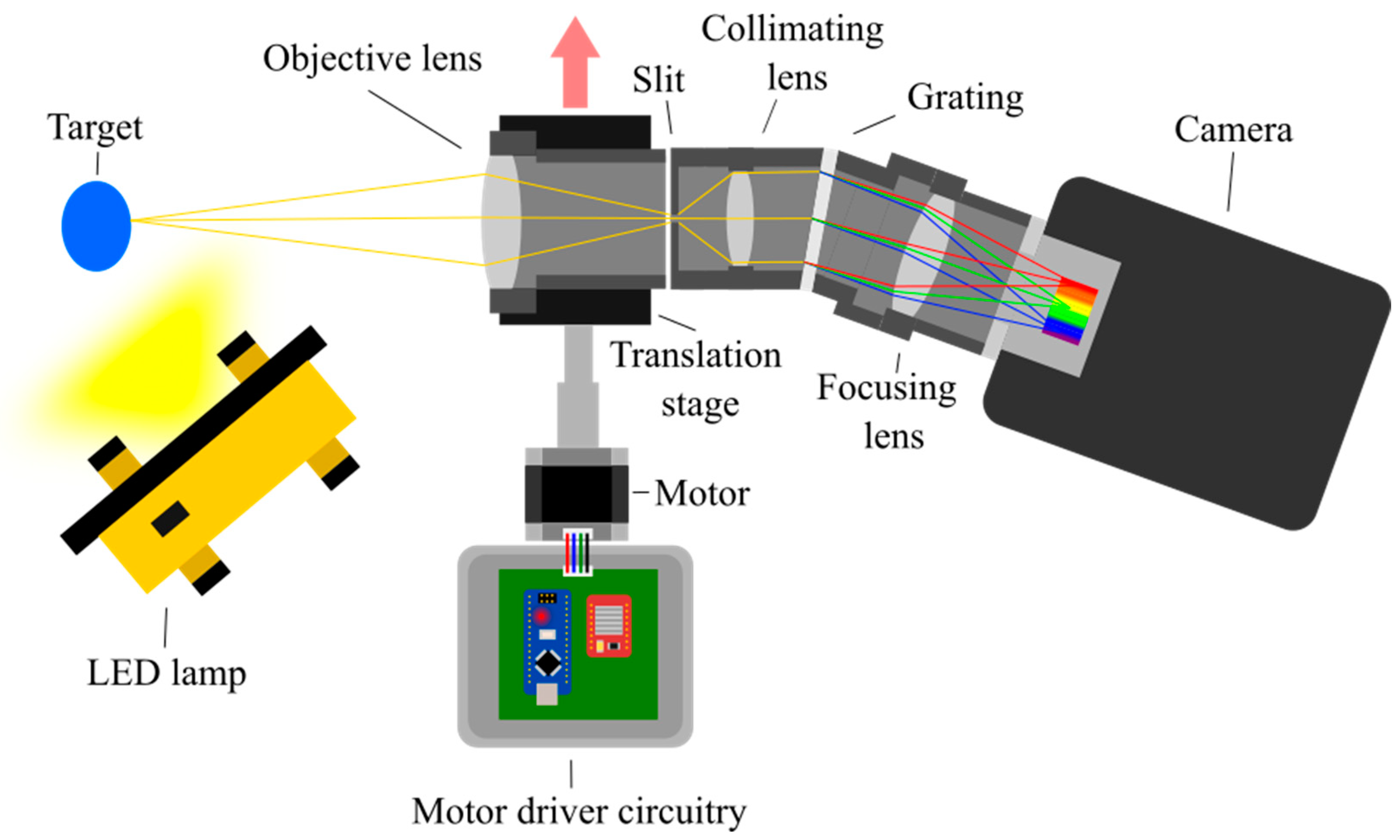
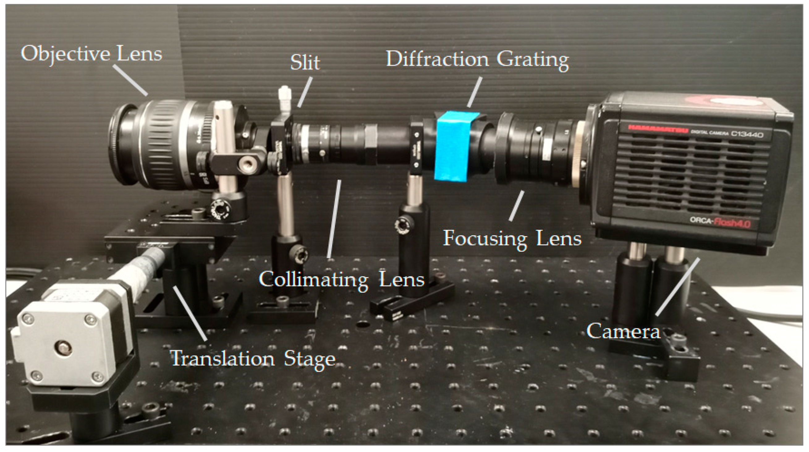
2. Materials and Methods
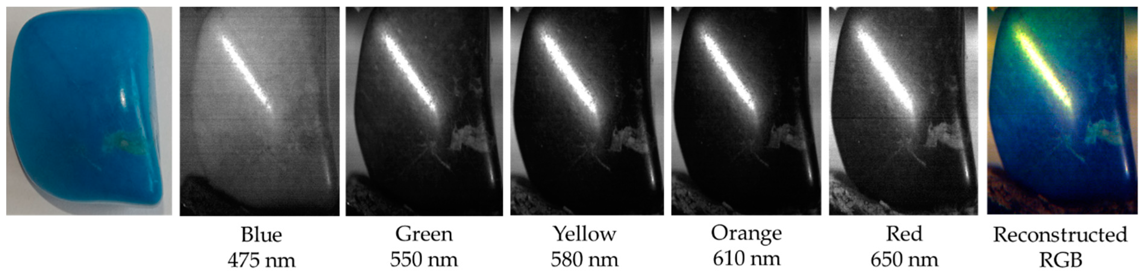
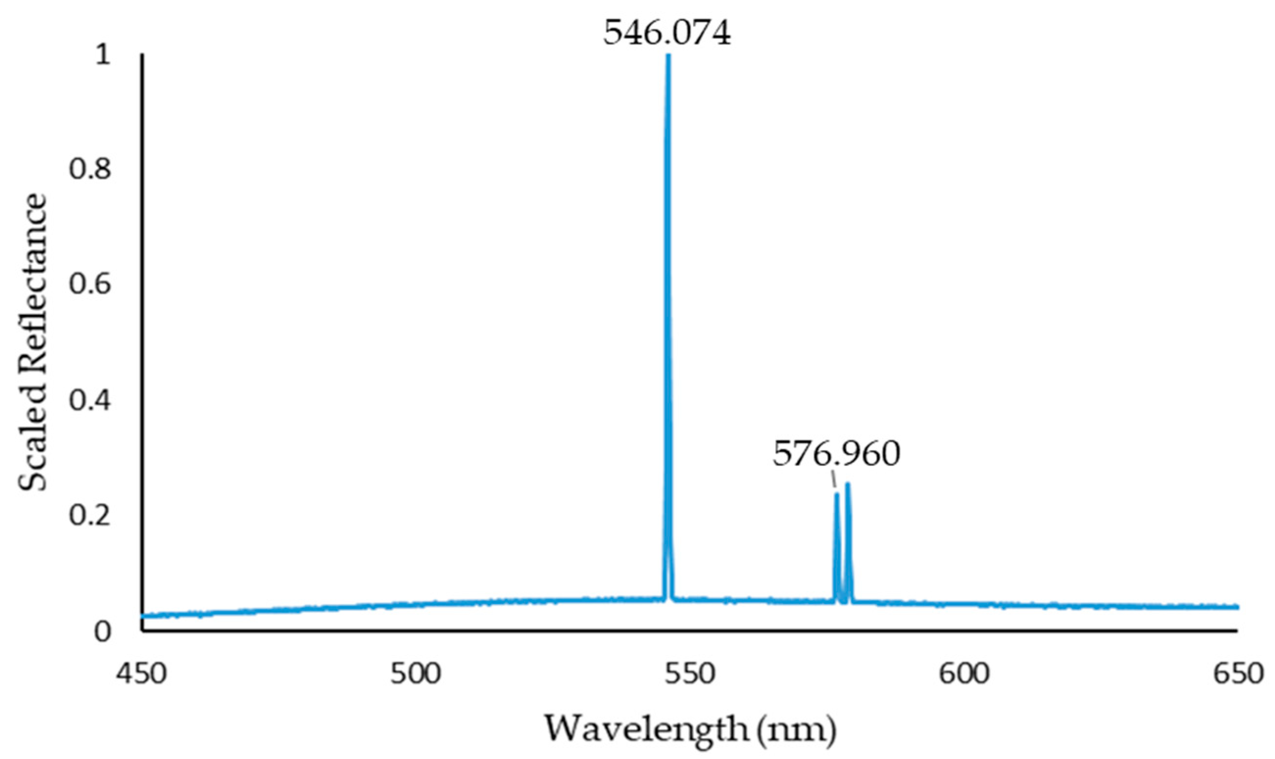
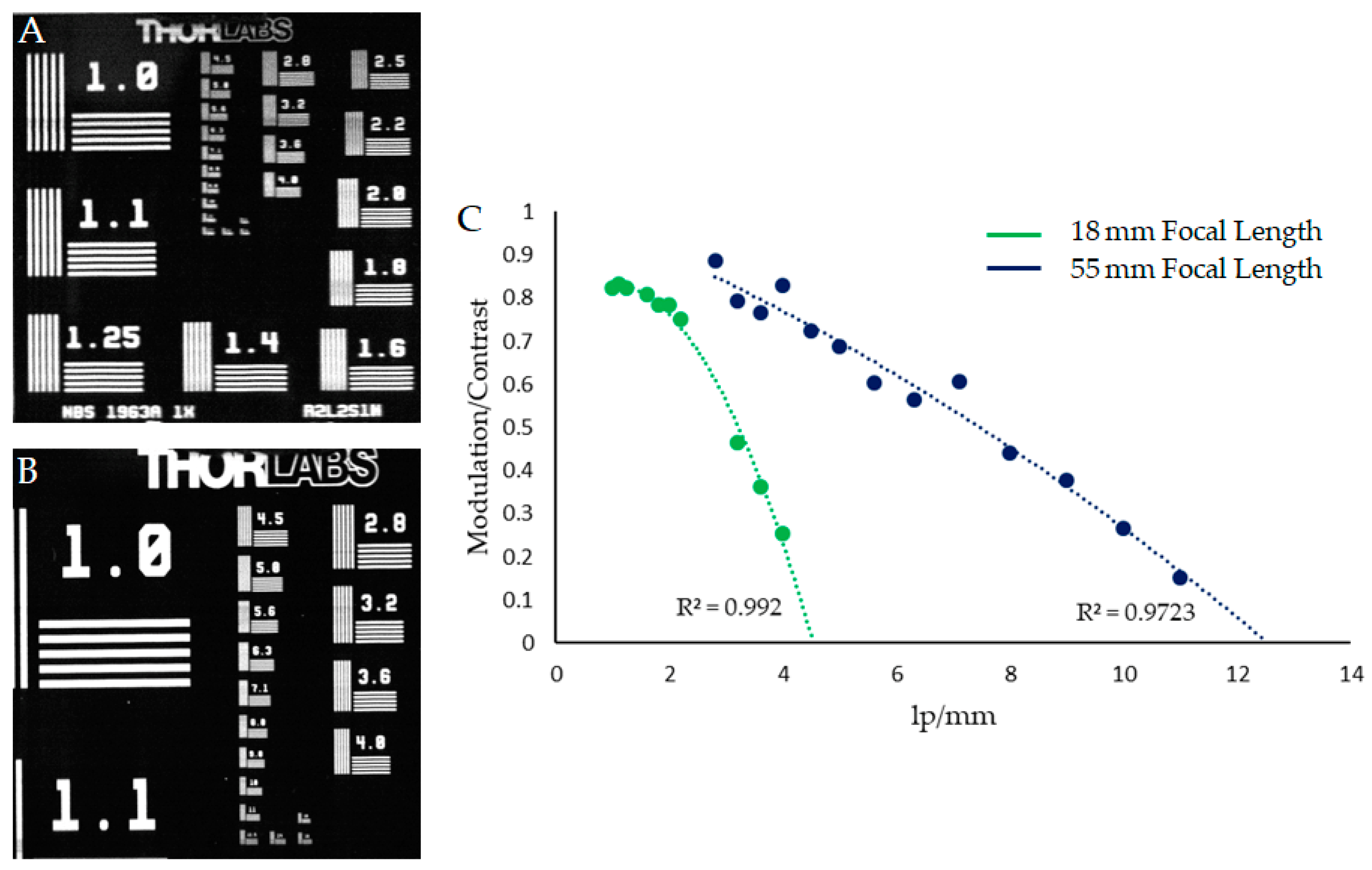
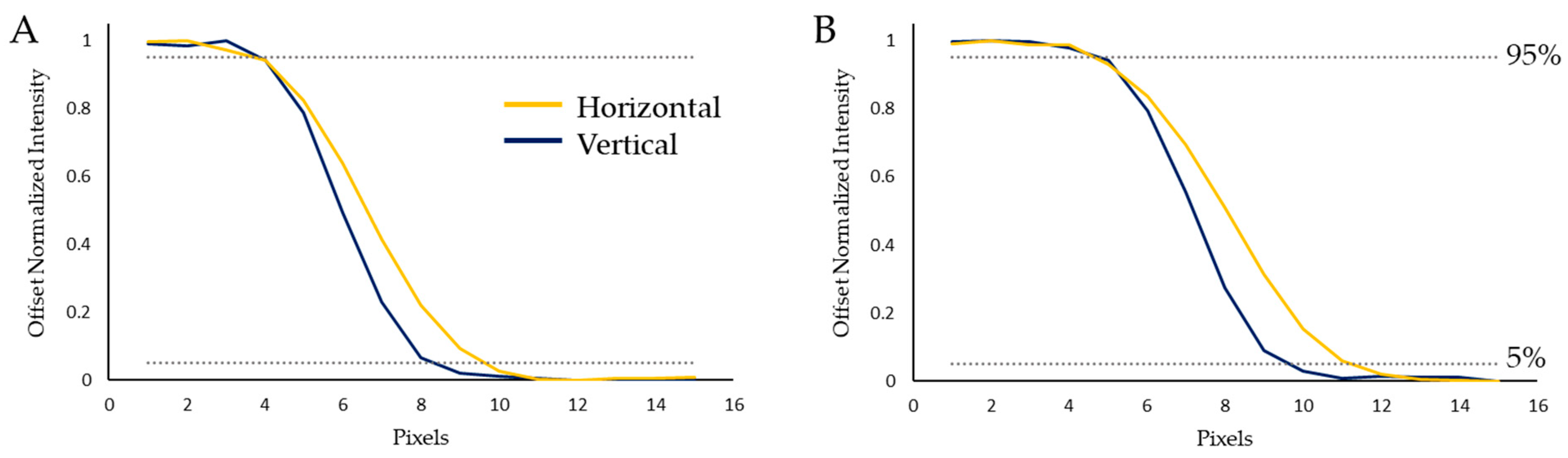
3. Results
Optical Characterisation
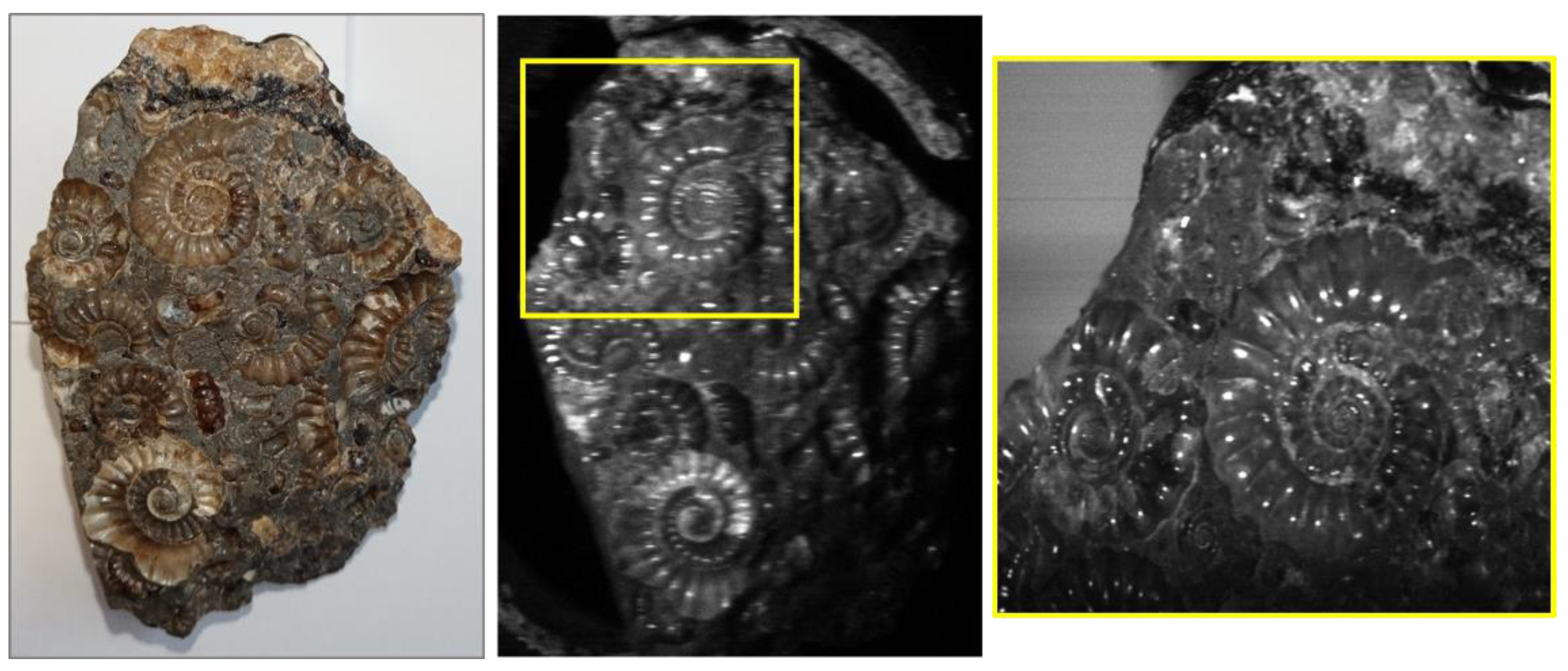
4. Discussion
Example Application
5. Conclusions
Author Contributions
Funding
Data Availability Statement
Conflicts of Interest
References
- Jia, J.; Chen, J.; Zheng, X.; Wang, Y.; Guo, S.; Sun, H.; Jiang, C.; Karjalainen, M.; Karila, K.; Duan, Z.; et al. Tradeoffs in the Spatial and Spectral Resolution of Airborne Hyperspectral Imaging Systems: A Crop Identification Case Study. IEEE Trans. Geosci. Remote Sens. 2021, 60, 5510918. [Google Scholar] [CrossRef]
- Jia, J.; Wang, Y.; Chen, J.; Guo, R.; Shu, R.; Wang, J. Status and application of advanced airborne hyperspectral imaging technology: A review. Infrared Phys. Technol. 2020, 104, 103115. [Google Scholar] [CrossRef]
- Yang, Q. Design study of a compact ultra-wide-angle high-spatial-resolution high-spectral-resolution snapshot imaging spectrometer. Opt. Express 2021, 29, 2893. [Google Scholar] [CrossRef]
- Brady, D.J. Optical Imaging and Spectroscopy; John Wiley & Sons: Hoboken, NJ, USA, 2009. [Google Scholar]
- Barducci, A.; Guzzi, D.; Lastri, C.; Nardino, V.; Marcoionni, P.; Pippi, I. Radiometric and signal-to-noise ratio properties of multiplex dispersive spectrometry. Appl. Opt. 2010, 49, 5366–5373. [Google Scholar] [CrossRef]
- Stuart, M.B.; McGonigle, A.J.S.; Willmott, J.R. Hyperspectral imaging in environmental monitoring: A review of recent developments and technological advances in compact field deployable systems. Sensors 2019, 19, 3071. [Google Scholar] [CrossRef] [PubMed] [Green Version]
- Stuart, M.B.; Stanger, L.R.; Hobbs, M.J.; Pering, T.D.; Thio, D.; McGonigle, A.J.S.; Willmott, J.R. Low-cost hyperspectral imaging system: Design and testing for laboratory-based environmental applications. Sensors 2020, 20, 3293. [Google Scholar] [CrossRef]
- Banerjee, B.P.; Raval, S.; Cullen, P.J. UAV-hyperspectral imaging of spectrally complex environments. Int. J. Remote Sens. 2020, 41, 4136–4159. [Google Scholar] [CrossRef]
- Wilkes, T.C.; Pering, T.D.; McGonigle, A.J.S.; Tamburello, G.; Willmott, J.R. A low-cost smartphone sensor-based UV camera for volcanic SO2 emission measurements. Remote Sens. 2017, 9, 27. [Google Scholar] [CrossRef] [Green Version]
- Adam, E.; Mutanga, O.; Rugege, D. Multispectral and hyperspectral remote sensing for identification and mapping of wetland vegetation: A review. Wetl. Ecol. Manag. 2010, 18, 281–296. [Google Scholar] [CrossRef]
- Zhang, J.; Rivard, B.; Sánchez-Azofeifa, A.; Castro-Esau, K. Intra- and inter-class spectral variability of tropical tree species at La Selva, Costa Rica: Implications for species identification using HYDICE imagery. Remote Sens. Environ. 2006, 105, 129–141. [Google Scholar] [CrossRef]
- Galieni, A.; Nicastro, N.; Pentangelo, A.; Platani, C.; Cardi, T.; Pane, C. Surveying soil-borne disease development on wild rocket salad crop by proximal sensing based on high-resolution hyperspectral features. Sci. Rep. 2022, 12, 5098. [Google Scholar] [CrossRef] [PubMed]
- Yang, G.; Huang, K.; Sun, W.; Meng, X.; Mao, D.; Ge, Y. Enhanced mangrove vegetation index based on hyperspectral images for mapping mangrove. ISPRS J. Photogramm. Remote Sens. 2022, 189, 236–254. [Google Scholar] [CrossRef]
- Ma, Y.; Zhang, Q.; Yi, X.; Ma, L.; Zhang, L.; Huang, C.; Zhang, Z.; Lv, X. Estimation of cotton leaf area index (LAI) based on spectral transformation and vegetation index. Remote Sens. 2022, 14, 136. [Google Scholar] [CrossRef]
- Barton, I.F.; Gabriel, M.J.; Lyons-Baral, J.; Barton, M.D.; Duplessis, L.; Roberts, C. Extending geometallurgy to the mine scale with hyperspectral imaging: A pilot study using drone- and ground-based scanning. Min. Metall. Explor. 2021, 38, 799–818. [Google Scholar] [CrossRef]
- Parbhaker-Fox, A.; Lottermoser, B.; Bradshaw, D.J. Cost-Effective Means for Identifying Acid Rock Drainage Risks—Integration of the Geochemistry- Mineralogy-Texture Approach and Geometallurgical Techniques. In Proceedings of the Second Ausimm International Geometallurgy Conference, Brisbane, Australia, 2 October 2013; pp. 143–154. [Google Scholar]
- Gallie, E.A.; McArdle, S.; Rivard, B.; Francis, H. Estimating sulphide ore grade in broken rock using visible/infrared hyperspectral reflectance spectra. Int. J. Remote Sens. 2002, 23, 2229–2246. [Google Scholar] [CrossRef]
- Kokaly, R.F.; Graham, G.E.; Hoefen, T.M.; Kelley, K.D.; Johnson, M.R.; Hubbard, B.E.; Buchhorn, M.; Prakash, A. Multiscale Hyperspectral Imaging of the Orange Hill Porphyry Copper Deposit, Alaska, USA, with Laboratory-, Field-, and Aircraft-based Imaging Spectrometers. Proc. Explor. 2017, 17, 923–943. [Google Scholar]
- van der Meer, F.D.; van der Werff, H.M.A.; van Ruitenbeek, F.J.A.; Hecker, C.A.; Bakker, W.H.; Noomen, M.F.; van der Meijde, M.; Carranza, J.M.; de Smeth, J.B.; Woldai, T. Multi- and hyperspectral geologic remote sensing: A review. Int. J. Appl. Earth Obs. Geoinf. 2012, 14, 112–128. [Google Scholar] [CrossRef]
- Sabins, F. Remote sensing for mineral exploration. Ore Geol. Rev. 1999, 14, 157–183. [Google Scholar] [CrossRef]
- Swayze, G.A.; Smith, K.S.; Clark, R.N.; Sutley, S.J.; Pearson, R.M.; Vance, J.S.; Hageman, P.L.; Briggs, P.H.; Meier, A.L.; Singleton, M.J.; et al. Using imaging spectroscopy to map acidic mine waste. Environ. Sci. Technol. 2000, 34, 47–54. [Google Scholar] [CrossRef]
- Shang, J.; Morris, B.; Howarth, P.; Lévesque, J.; Staenz, K.; Neville, B. Mapping mine tailing surface mineralogy using hyperspectral remote sensing. Can. J. Remote Sens. 2009, 35, S126–S141. [Google Scholar] [CrossRef]
- Nikonow, W.; Rammlmair, D.; Meima, J.A.; Schodlok, M.C. Advanced mineral characterization and petrographic analysis by μ-EDXRF, LIBS, HSI and hyperspectral data merging. Mineral. Petrol. 2019, 113, 417–431. [Google Scholar] [CrossRef]
- Roy, S.; Bhattacharya, S.; Omkar, S.N. Automated large-scale mapping of the Jahazpur mineralized belt by a MapReduce model with an integrated ELM method. PFG—J. Photogramm. Remote Sens. Geoinf. Sci. 2022, 90, 191–209. [Google Scholar] [CrossRef]
- Iqbal, M.A.; Rezaee, R.; Laukamp, C.; Pejcic, B.; Smith, G. Integrated sedimentary and high-resolution mineralogical characterization of Ordovician shale from Canning Basin, Western Australia: Implications for facies heterogeneity evaluation. J. Pet. Sci. Eng. 2021, 208, 109347. [Google Scholar] [CrossRef]
- Lombi, E.; De Jonge, M.D.; Donner, E.; Ryan, C.G.; Paterson, D. Trends in hard X-ray fluorescence mapping: Environmental applications in the age of fast detectors. Anal. Bioanal. Chem. 2011, 400, 1637–1644. [Google Scholar] [CrossRef]
- Belissont, R.; Muñoz, M.; Boiron, M.C.; Luais, B.; Mathon, O. Distribution and oxidation state of Ge, Cu and Fe in sphalerite by μ-XRF and K-edge μ-XANES: Insights into Ge incorporation, partitioning and isotopic fractionation. Geochim. Cosmochim. Acta 2016, 177, 298–314. [Google Scholar] [CrossRef]
- Flude, S.; Storey, M. 40Ar/39Ar age of the Rotoiti Breccia and Rotoehu Ash, Okataina Volcanic Complex, New Zealand, and identification of heterogeneously distributed excess 40Ar in supercooled crystals. Quat. Geochronol. 2016, 33, 13–23. [Google Scholar] [CrossRef] [Green Version]
- Melcher, F.; Oberthür, T.; Rammlmair, D. Geochemical and mineralogical distribution of germanium in the Khusib Springs Cu-Zn-Pb-Ag sulfide deposit, Otavi Mountain Land, Namibia. Ore Geol. Rev. 2006, 28, 32–56. [Google Scholar] [CrossRef]
- Bower, D.M.; Yang, C.S.C.; Hewagama, T.; Nixon, C.A.; Aslam, S.; Whelley, P.L.; Eigenbrode, J.L.; Jin, F.; Ruliffson, J.; Kolasinski, J.R.; et al. Spectroscopic characterization of samples from different environments in a Volcano-Glacial region in Iceland: Implications for in situ planetary exploration. Spectrochim. Acta Part A Mol. Biomol. Spectrosc. 2021, 263, 120205. [Google Scholar] [CrossRef]
- Amici, S.; Piscini, A.; Neri, M. Reflectance Spectra Measurements of Mt. Etna: A Comparison with Multispectral/Hyperspectral Satellite. Adv. Remote Sens. 2014, 3, 235–245. [Google Scholar] [CrossRef] [Green Version]
- Capaccioni, F.; Bellucci, G.; Orosei, R.; Amici, S.; Bianchi, R.; Blecka, M.; Capria, M.T.; Coradini, A.; Erard, S.; Fonti, S.; et al. Mars-IRMA: In-situ infrared microscope analysis of Martian soil and rock samples. Adv. Space Res. 2001, 28, 1219–1224. [Google Scholar] [CrossRef]
- Sgavetti, M.; Pompilio, L.; Roveri, M.; Manzi, V.; Valentino, G.M.; Lugli, S.; Carli, C.; Amici, S.; Marchese, F.; Lacava, T. Two geologic systems providing terrestrial analogues for the exploration of sulfate deposits on Mars: Initial spectral characterization. Planet. Space Sci. 2009, 57, 614–627. [Google Scholar] [CrossRef]
- Amici, S.; Piscini, A.; Buongiorno, M.F.; Pieri, D. Geological classification of Volcano Teide by hyperspectral and multispectral satellite data. Int. J. Remote Sens. 2013, 34, 3356–3375. [Google Scholar] [CrossRef]
- Gadd, G.M. Metals, minerals and microbes: Geomicrobiology and bioremediation. Microbiology 2010, 156, 609–643. [Google Scholar] [CrossRef] [PubMed]
- Zhu, C.; Hobbs, M.J.; Masters, R.C.; Rodenburg, C.; Willmott, J.R. An accurate device for apparent emissivity characterization in controlled atmospheric conditions up to 1423 K. IEEE Trans. Instrum. Meas. 2020, 69, 4210–4221. [Google Scholar] [CrossRef]
- Stanger, L.; Rockett, T.; Lyle, A.; Davies, M.; Anderson, M.; Todd, I.; Basoalto, H.; Willmott, J.R. Reconstruction of microscopic thermal fields from oversampled infrared images in laser-based powder bed fusion. Sensors 2021, 21, 4859. [Google Scholar] [CrossRef]
- Davies, M.; Stuart, M.B.; Hobbs, M.; McGonigle, A.; Willmott, J.R. Image Correction and In-Situ Spectral Calibration for Low-Cost Smartphone Hyperspectral Imaging. Remote Sens. 2022, 14, 1152. [Google Scholar] [CrossRef]


| Component | Part Used |
|---|---|
| Objective Lens | Canon EF-S 18–55 mm |
| Slit | Thorlabs VA100C (set at 300 μm). |
| Collimating Lens | Thorlabs MVL75M1 75 mm telephoto c mount |
| Transmission Diffraction Grating | Edmund Optics #49-580 |
| Focusing Lens | Thorlabs MVL50M23 50 mm telephoto c mount |
| Camera Sensor | Hamamatsu C13440 |
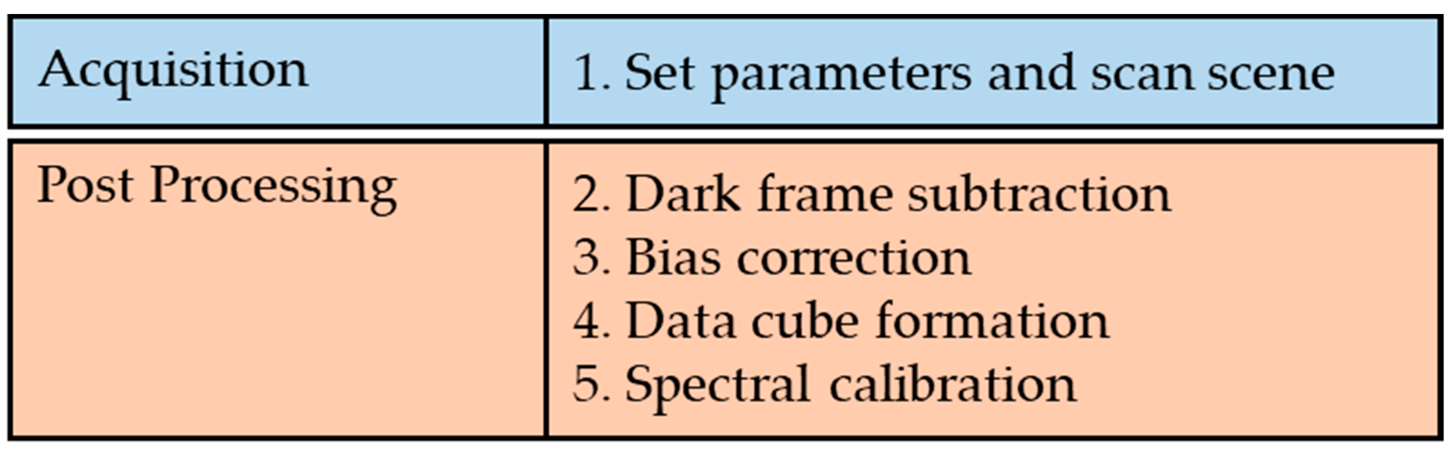
| Setting | |
|---|---|
| Exposure Time (ms) | 60 |
| Wavelength Range (nm) | 450–650 |
| Spectral Resolution (FWHM) (nm) | 0.29 |
| Spatial Resolution (pixels) | 1000 × 1000 |
| Focal Lengths (mm) | 18 and 55 |
Publisher’s Note: MDPI stays neutral with regard to jurisdictional claims in published maps and institutional affiliations. |
© 2022 by the authors. Licensee MDPI, Basel, Switzerland. This article is an open access article distributed under the terms and conditions of the Creative Commons Attribution (CC BY) license (https://creativecommons.org/licenses/by/4.0/).
Share and Cite
Stuart, M.B.; Davies, M.; Hobbs, M.J.; Pering, T.D.; McGonigle, A.J.S.; Willmott, J.R. High-Resolution Hyperspectral Imaging Using Low-Cost Components: Application within Environmental Monitoring Scenarios. Sensors 2022, 22, 4652. https://doi.org/10.3390/s22124652
Stuart MB, Davies M, Hobbs MJ, Pering TD, McGonigle AJS, Willmott JR. High-Resolution Hyperspectral Imaging Using Low-Cost Components: Application within Environmental Monitoring Scenarios. Sensors. 2022; 22(12):4652. https://doi.org/10.3390/s22124652
Chicago/Turabian StyleStuart, Mary B., Matthew Davies, Matthew J. Hobbs, Tom D. Pering, Andrew J. S. McGonigle, and Jon R. Willmott. 2022. "High-Resolution Hyperspectral Imaging Using Low-Cost Components: Application within Environmental Monitoring Scenarios" Sensors 22, no. 12: 4652. https://doi.org/10.3390/s22124652
APA StyleStuart, M. B., Davies, M., Hobbs, M. J., Pering, T. D., McGonigle, A. J. S., & Willmott, J. R. (2022). High-Resolution Hyperspectral Imaging Using Low-Cost Components: Application within Environmental Monitoring Scenarios. Sensors, 22(12), 4652. https://doi.org/10.3390/s22124652