
Multivariate Time Series Deep Spatiotemporal Forecasting with Graph Neural Network


Abstract
:1. Introduction
- 1.
- A more general time series forecasting model based on graph convolutional networks and deep spatiotemporal features is proposed in this paper.
- 2.
- The attention mechanism is added to the graph convolution module to realize the filtering of spatiotemporal information.
- 3.
- A down-sampling convolution module is proposed to extract deep spatiotemporal information of time series to improve the performance of the model.
2. Related Works
2.1. Time Series Forecasting with Traditional Methods
2.2. Time Series Forecasting with Deep Learning
3. Methods
3.1. Problem Definition
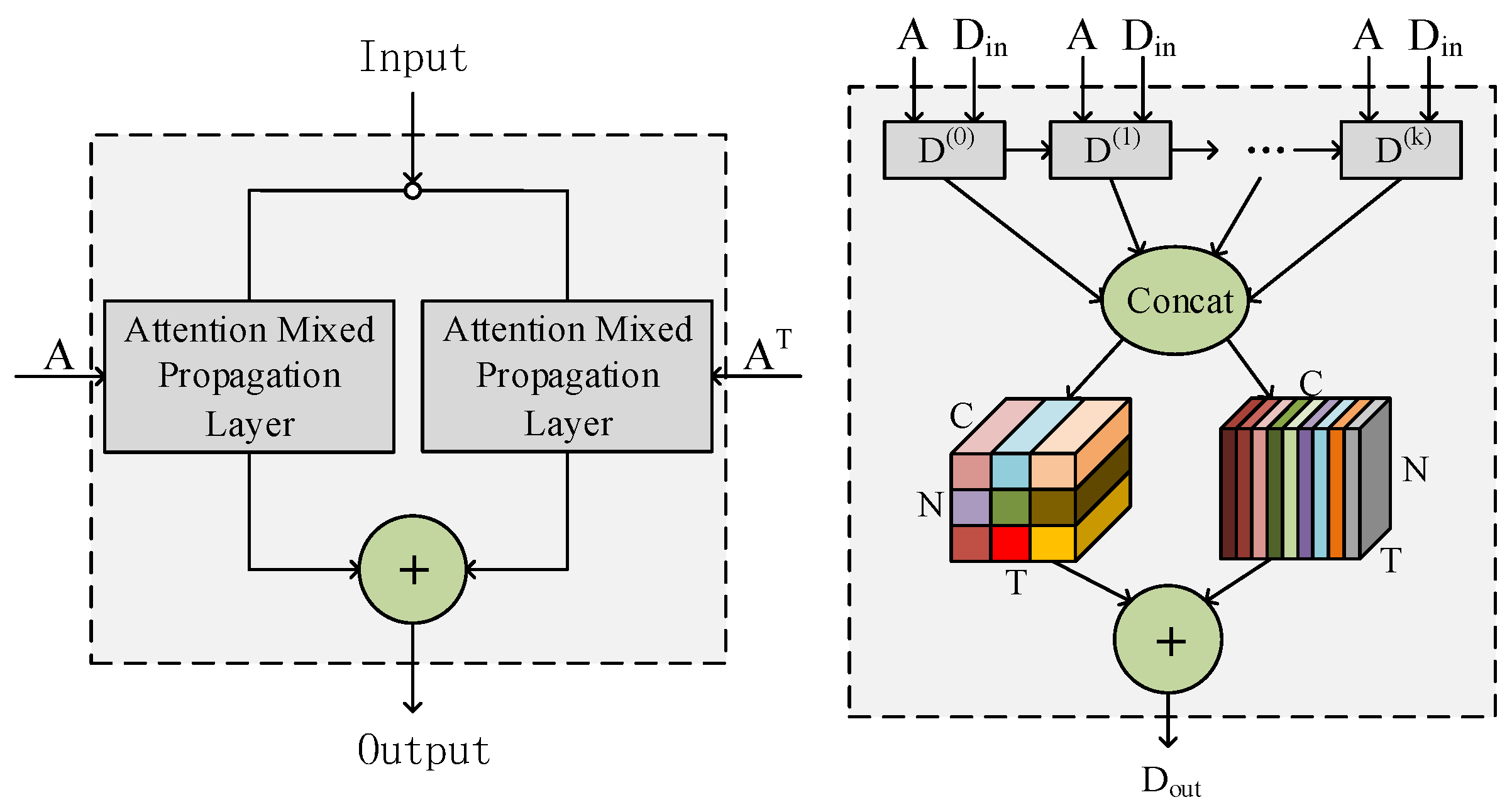
3.2. Graph Learning Module
3.3. Temporal Convolution Module
3.4. Graph Convolution Module
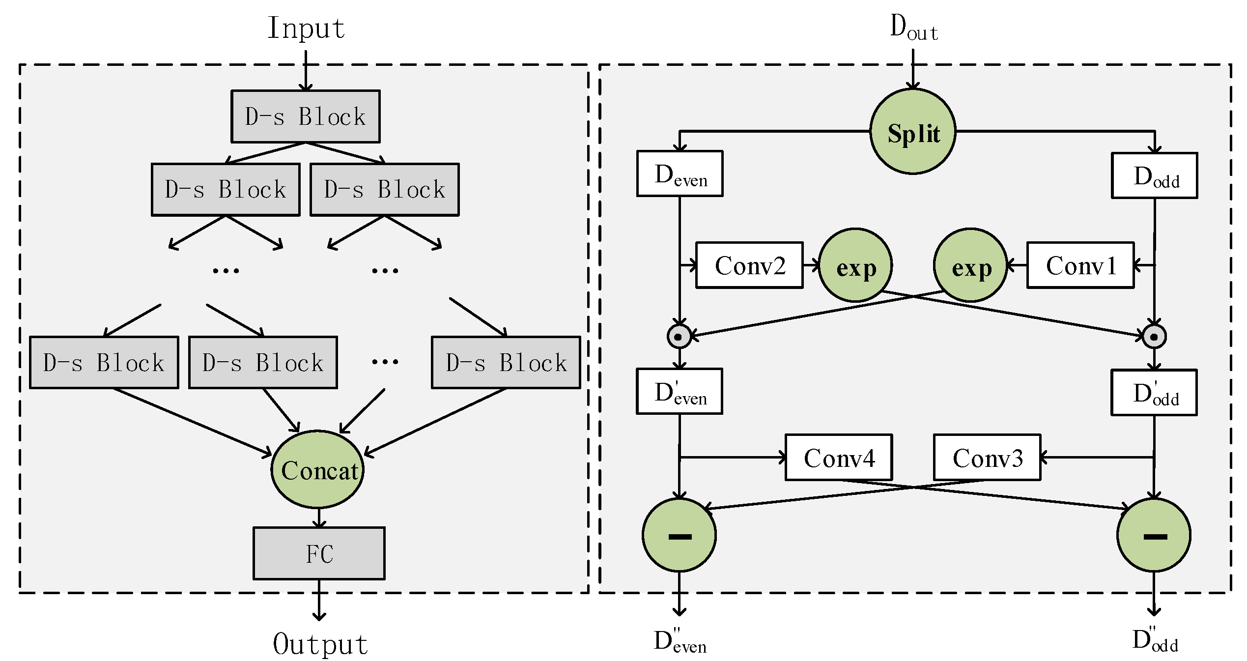
3.5. Down-Sampling Convolution Module
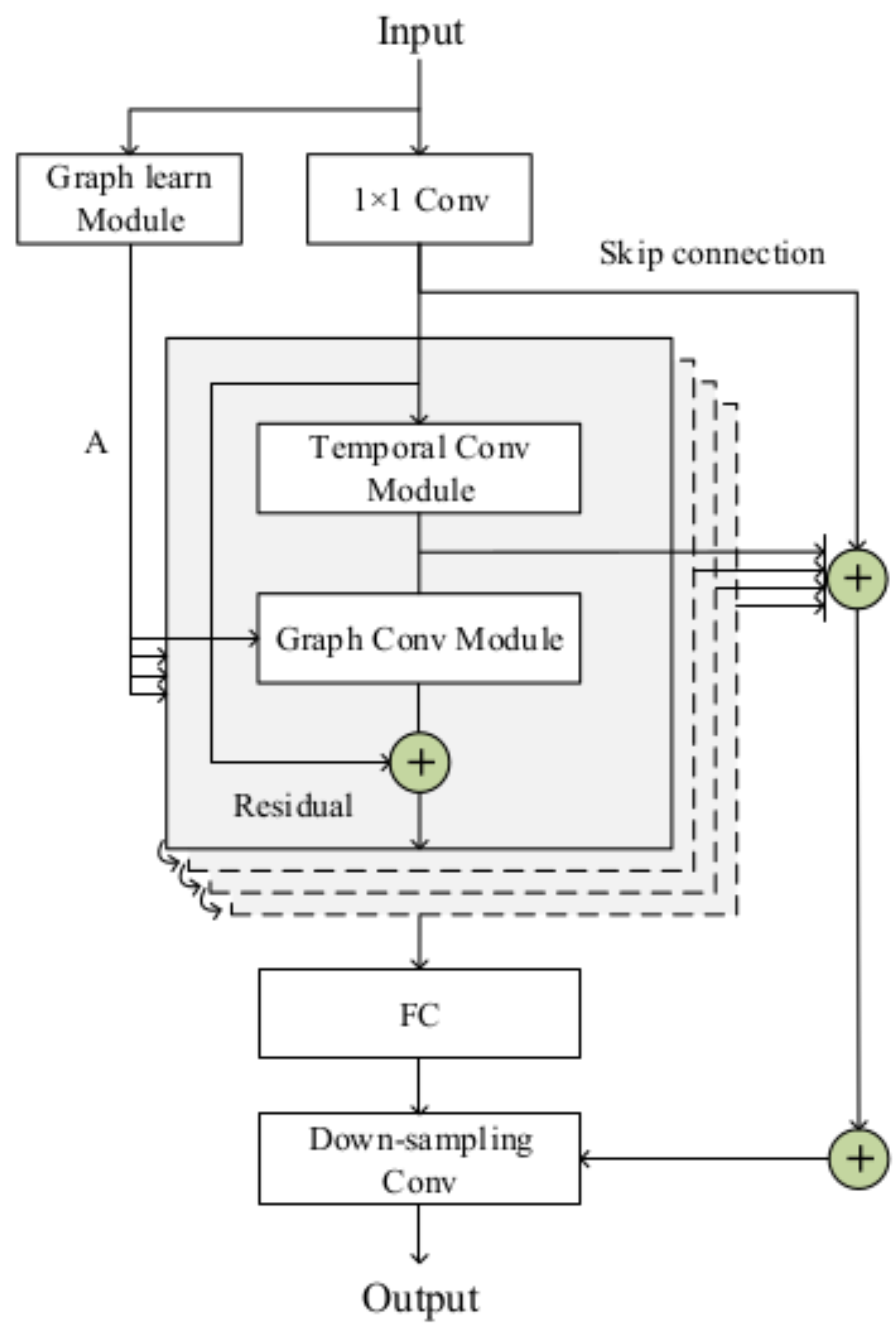
3.6. Experiment Model
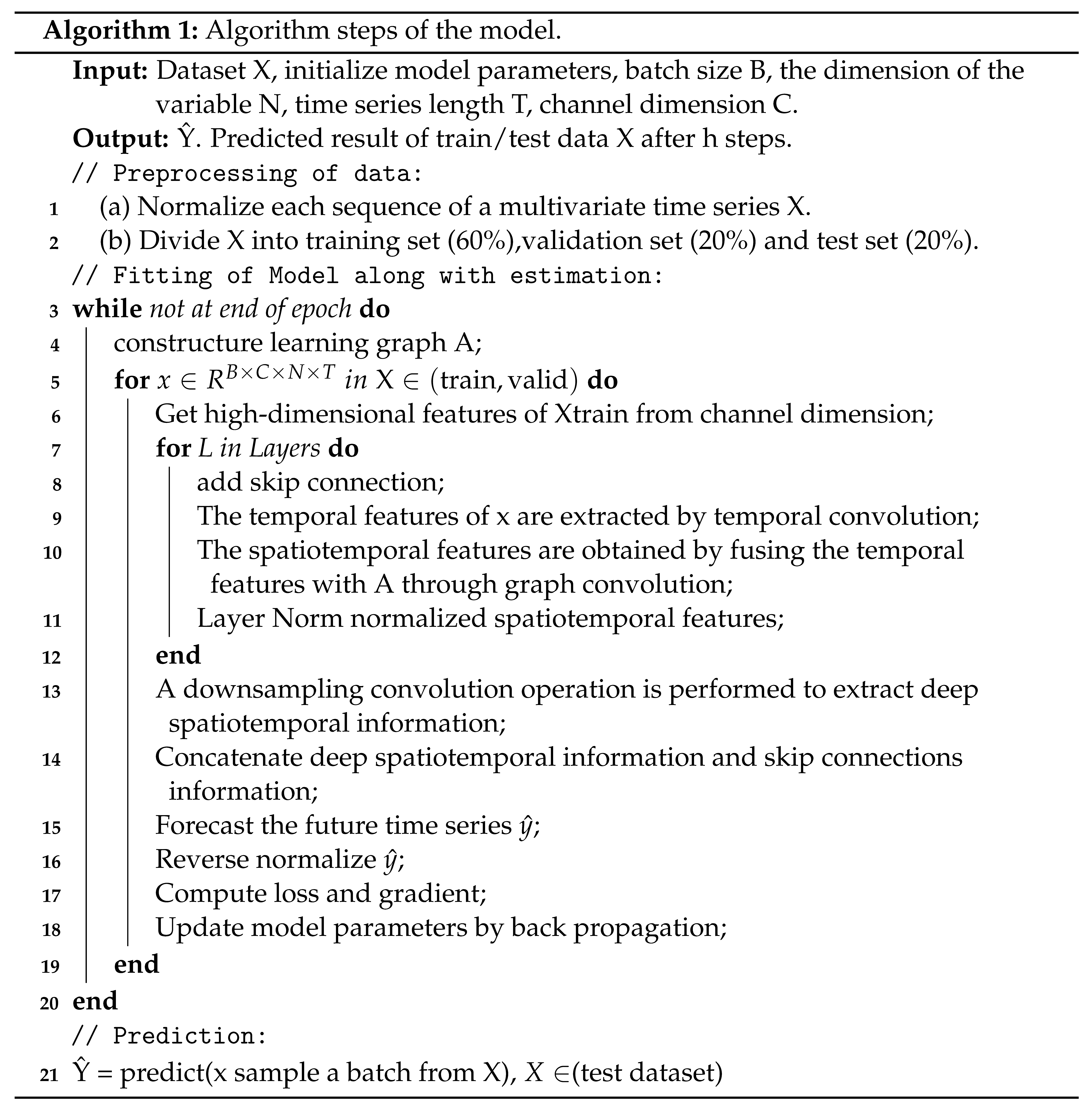
- Input: The raw data X of the multivariate time series.
- Output: The prediction result of data X after h (Horizon) steps. The value of h can take 3, 6, 12, and 24.
- Line 1–2: Preprocess the input raw data X. Normalize each sequence of a multivariate time series X. Divide X into training set (60%), validation set (20%), and test set (20%). The Xtrain and Ytrain are obtained by splitting the sequence X with a fixed-length sliding window. Xtrain represents the input data for training, and Ytrain represents the labels of the training data.
- Line 4: Construct the graph structure A of the multivariate time series. A represents the dependencies between different sequences in a multivariate time series by an adjacency matrix.
- Line 6: A 1 × 1 convolutional network is used to obtain high-dimensional data in the channel dimension of Xtrain.
- Line 8: Add skip connection method to preserve part of the original information of each layer.
- Line 9: Perform a temporal convolution operation on the input data to obtain the temporal information of the data.
- Line 10: In the graph convolution, spatially weighted spatiotemporal information is obtained by multiplying the temporal information with an adjacency matrix A.
- Line 11: The output data are normalized using Layer Norm. Repeat Line 8 to Step 11 for L times. L represents the number of layers of the module.
- Line 13: Perform down-sampling convolution operation on the obtained spatiotemporal information to extract deep spatiotemporal information.
- Line 14–15: Concatenate deep spatiotemporal information and skip connections information. The final output result is obtained through 1 × 1 convolutional dimensionality reduction information.
- Line 16–18: Reverse normalize the output of the model. The mean value (MAE) of the difference between the output and the true value is used as the loss function. The model parameters are updated according to the gradient, and the steps from Step 3 to Step 10 are repeated until the model finally converges to the minimum error.
- Line 21: Finally, input the test set into the trained model to obtain the prediction result.
4. Experiment Analysis
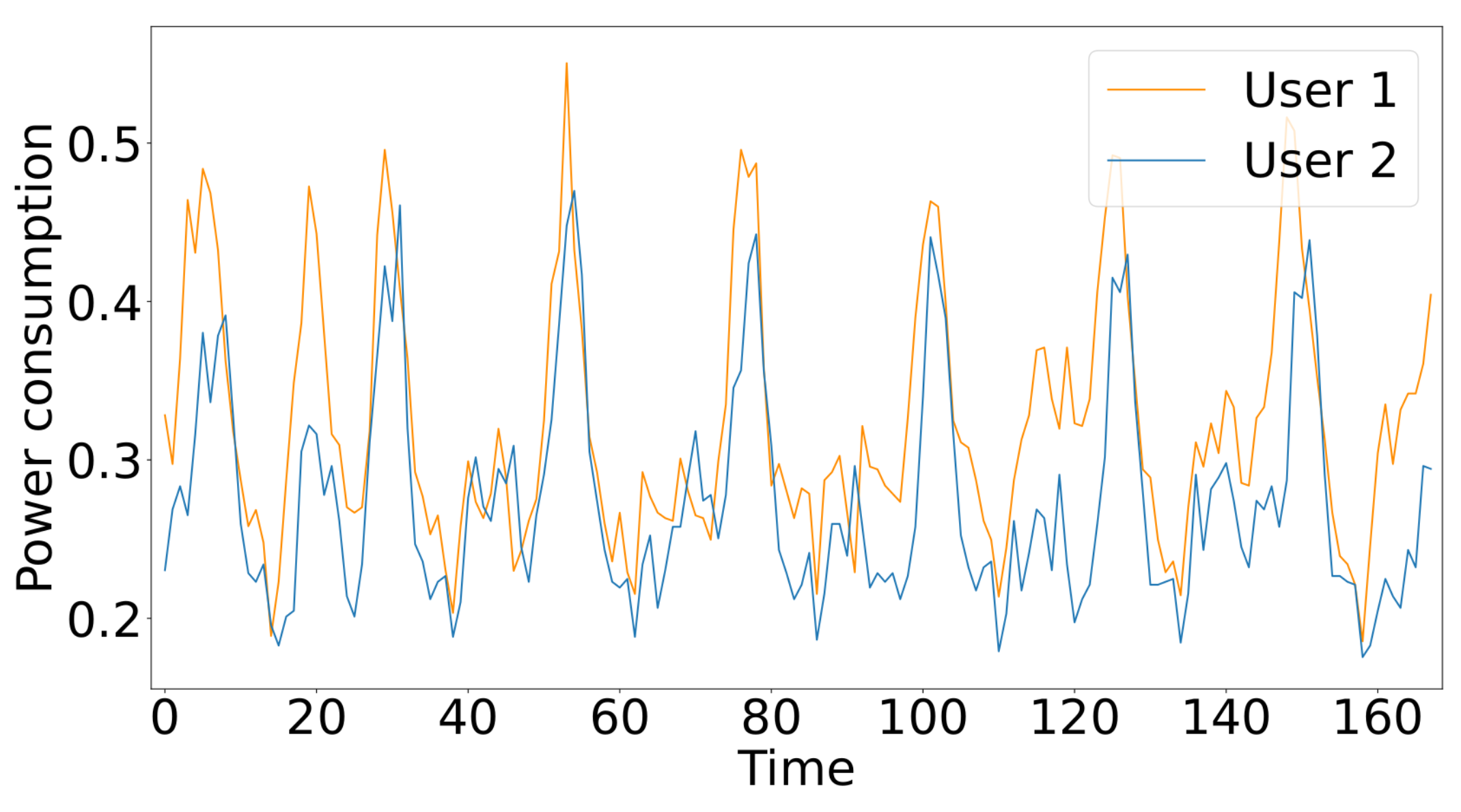
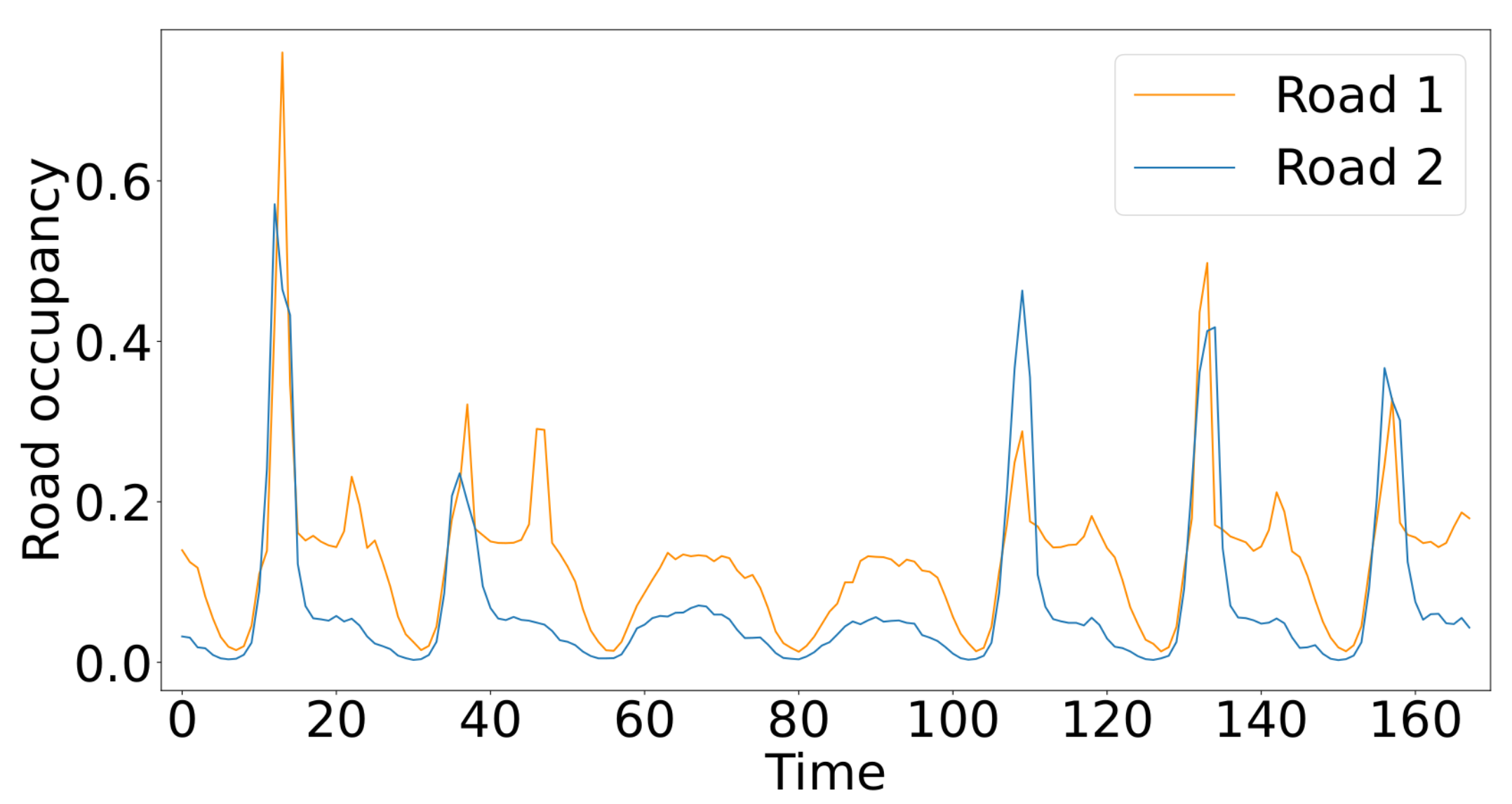
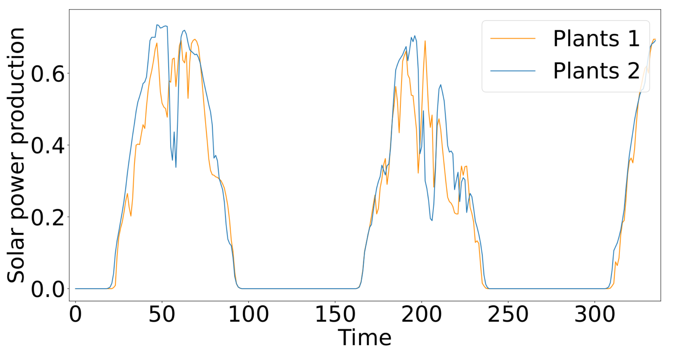
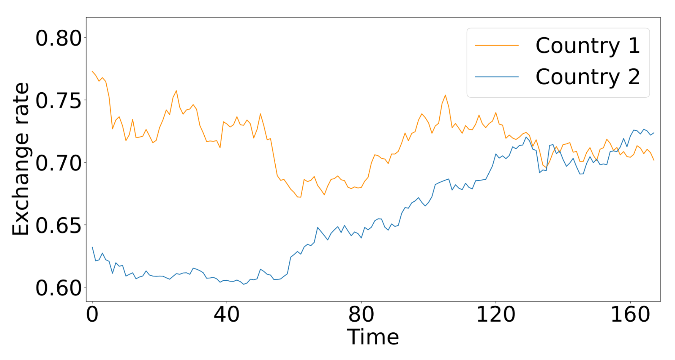
4.1. Experiment Dataset Analysis
- Solar Energy: Solar power generation data from Alabama State PV plants in 2006, sampled every 10 min from 137 PV plants;
- Traffic: Hourly road occupancy (between 0 and 1) on San Francisco Bay Area highways for 48 months (2015–2016) recorded by the California Department of Transportation, including data from 862 sensor measurements;
- Electricity: The hourly electricity consumption (kWh) of 321 users from 2012 to 2014;
- Exchange Rate: Daily exchange rate records for 8 countries (Australia, British, Canada, China, Japan, New Zealand, Singapore, and Switzerland) from 1990 to 2016.
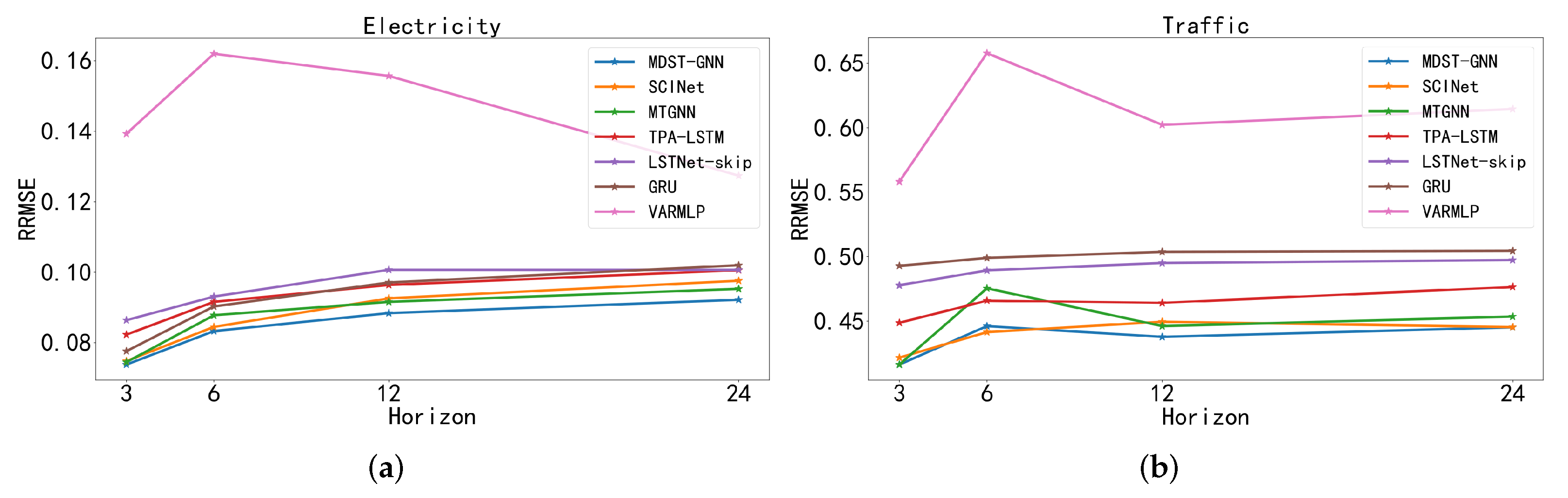
4.2. Methods for Comparison
- VAR-MLP: Hybrid model of multilayer perceptron (MLP) and autoregressive model (VAR) [13];
- GRU: Variant GRU model based on long short-term memory network;
- LSTNet: A hybrid model of deep neural network composed of convolutional neural network and recurrent neural network [19];
- TPA-LSTM: Recurrent Neural Network Model Based on Attention Mechanism [20];
- MTGNN: Hybrid model based on graph neural network and convolutional neural network [31];
- SCINet: Convolutional neural network model based on parity sequence segmentation and intersection [22].
4.3. Metrics
4.4. Experimental Setup
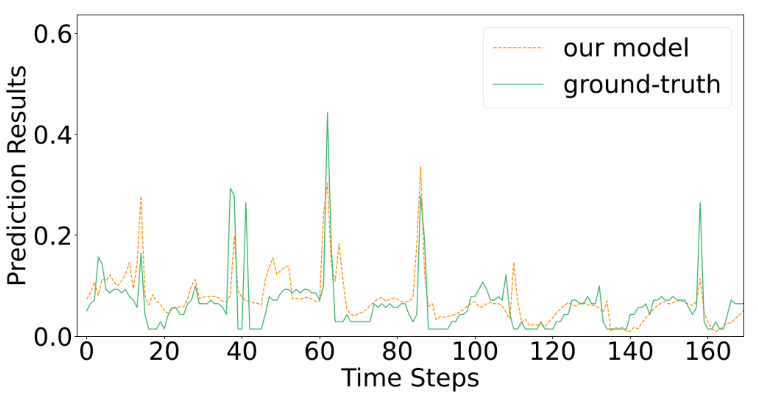
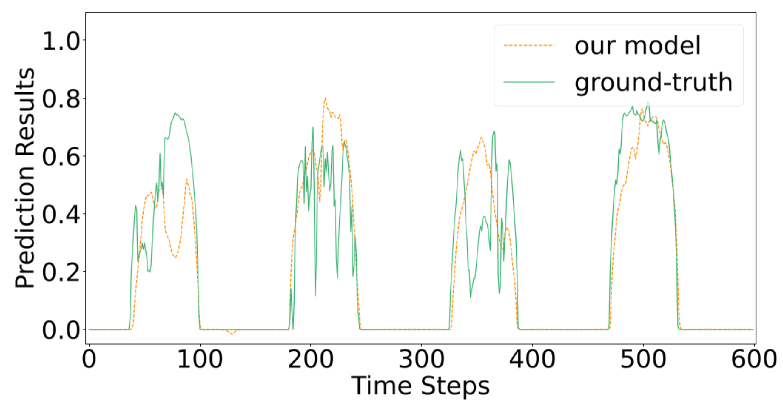
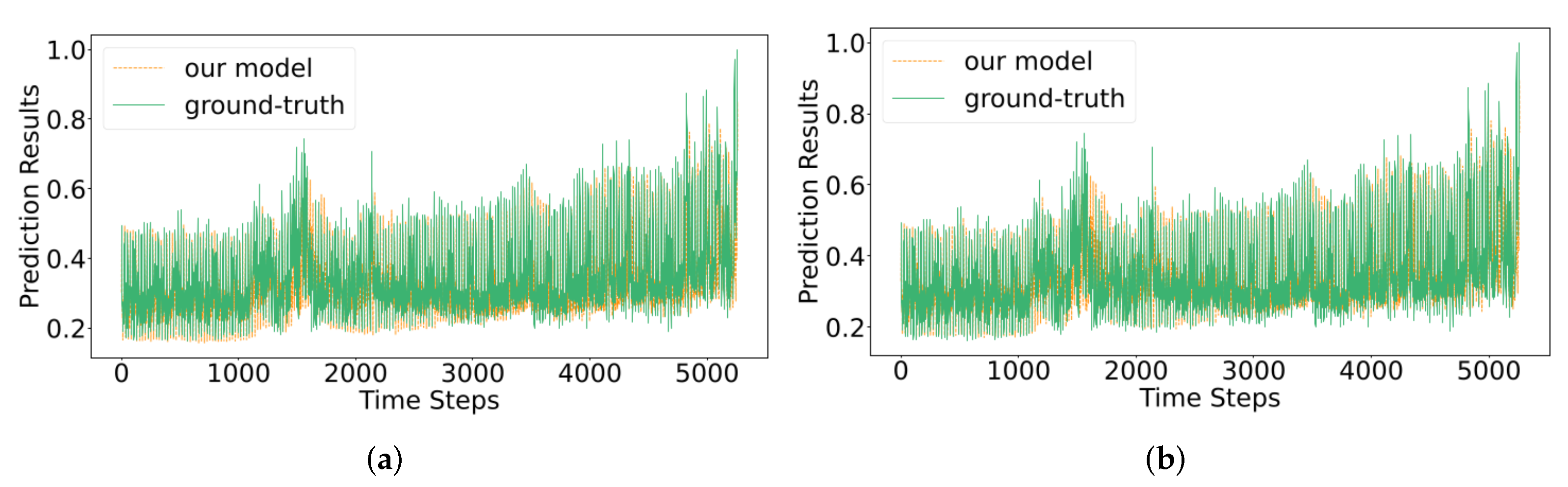
4.5. Results
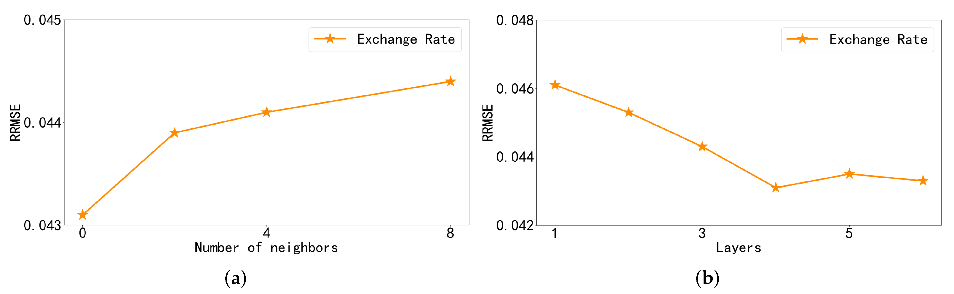
4.6. Ablation Study
- w/o A: The attention mechanism part is removed from the information selection process of the graph convolution module. The output of the information selection step is passed directly to the next section.
- w/o S: Remove the down-sampling convolution module from the model and replace that part with a fully connected layer.
5. Conclusions
Author Contributions
Funding
Institutional Review Board Statement
Informed Consent Statement
Data Availability Statement
Conflicts of Interest
References
- Taylor, J.W.; McSharry, P.E. Short-Term Load Forecasting Methods: An Evaluation Based on European Data. IEEE Trans. Power Syst. 2007, 22, 2213–2219. [Google Scholar] [CrossRef] [Green Version]
- Du, S.; Li, T.; Yang, Y.; Horng, S.J. Deep Air Quality Forecasting Using Hybrid Deep Learning Framework. IEEE Trans. Knowl. Data Eng. 2021, 33, 2412–2424. [Google Scholar] [CrossRef] [Green Version]
- Chen, J.L.; Li, G.; Wu, D.C.; Shen, S. Forecasting Seasonal Tourism Demand Using a Multiseries Structural Time Series Method. J. Travel Res. 2019, 58, 92–103. [Google Scholar] [CrossRef]
- Zhuang, D.E.H.; Li, G.C.L.; Wong, A.K.C. Discovery of Temporal Associations in Multivariate Time Series. IEEE Trans. Knowl. Data Eng. 2014, 26, 2969–2982. [Google Scholar] [CrossRef]
- Akdi, Y.; Glveren, E.; Nlü, K.; Yücel, M. Modeling and forecasting of monthly PM 2.5 emission of Paris by periodogram-based time series methodology. Environ. Monit. Assess. 2021, 193, 622. [Google Scholar] [CrossRef] [PubMed]
- Box, G.E.P.; Jenkins, G.M.; MacGregor, J.F. Some Recent Advances in Forecasting and Control. J. R. Stat. Soc. Ser. Appl. Stat. 1974, 23, 158–179. [Google Scholar] [CrossRef]
- Chouhan, V.; Singh, S.K.; Khamparia, A.; Gupta, D.; Tiwari, P.; Moreira, C.; Damaševičius, R.; de Albuquerque, V.H.C. A Novel Transfer Learning Based Approach for Pneumonia Detection in Chest X-ray Images. Appl. Sci. 2020, 10, 559. [Google Scholar] [CrossRef] [Green Version]
- Lin, T.H.; Akamatsu, T.; Tsao, Y. Sensing ecosystem dynamics via audio source separation: A case study of marine soundscapes off northeastern Taiwan. PLoS Comput. Biol. 2021, 17, e1008698. [Google Scholar] [CrossRef] [PubMed]
- Li, Q.; Li, S.; Zhang, S.; Hu, J.; Hu, J. A Review of Text Corpus-Based Tourism Big Data Mining. Appl. Sci. 2019, 9, 3300. [Google Scholar] [CrossRef] [Green Version]
- Li, G.; Nguyen, T.H.; Jung, J.J. Traffic Incident Detection Based on Dynamic Graph Embedding in Vehicular Edge Computing. Appl. Sci. 2021, 11, 5861. [Google Scholar] [CrossRef]
- Simeunovic, J.; Schubnel, B.; Alet, P.J.; Carrillo, R.E. Spatio-Temporal Graph Neural Networks for Multi-Site PV Power Forecasting. IEEE Trans. Sustain. Energy 2022, 13, 1210–1220. [Google Scholar] [CrossRef]
- Abbasimehr, H.; Paki, R. Improving time series forecasting using LSTM and attention models. J. Ambient Intell. Humaniz. Comput. 2022, 13, 673–691. [Google Scholar] [CrossRef]
- Zhang, G. Time series forecasting using a hybrid ARIMA and neural network model. Neurocomputing 2003, 50, 159–175. [Google Scholar] [CrossRef]
- Zhang, G.; Patuwo, B.E.; Hu, M.Y. Forecasting with artificial neural networks: The state of the art. Int. J. Forecast. 1998, 14, 35–62. [Google Scholar] [CrossRef]
- Kaur, T.; Kumar, S.; Segal, R. Application of artificial neural network for short term wind speed forecasting. In Proceedings of the 2016 Biennial International Conference on Power and Energy Systems: Towards Sustainable Energy (PESTSE), Bengaluru, India, 21–23 January 2016; pp. 1–5. [Google Scholar] [CrossRef]
- Bukhari, A.H.; Raja, M.A.Z.; Sulaiman, M.; Islam, S.; Shoaib, M.; Kumam, P. Fractional Neuro-Sequential ARFIMA-LSTM for Financial Market Forecasting. IEEE Access 2020, 8, 71326–71338. [Google Scholar] [CrossRef]
- Cao, L.J.; Tay, F.E.H. Support vector machine with adaptive parameters in financial time series forecasting. IEEE Trans. Neural Netw. 2003, 14, 1506–1518. [Google Scholar] [CrossRef] [Green Version]
- Qin, D. Rise of VAR modelling approach. J. Econ. Surv. 2011, 25, 156–174. [Google Scholar] [CrossRef]
- Lai, G.K.; Chang, W.C.; Yang, Y.M.; Liu, H.X. Modeling Long–Short-Term Temporal Patterns with Deep Neural Networks. In Proceedings of the 41st International ACM SIGIR Conference on Research and Development in Information Retrieval, Ann Arbor, MI, USA, 8–12 July 2018; pp. 95–104. [Google Scholar] [CrossRef] [Green Version]
- Shih, S.Y.; Sun, F.K.; Lee, H.Y. Temporal pattern attention for multivariate time series forecasting. Mach. Learn. 2019, 108, 1421–1441. [Google Scholar] [CrossRef] [Green Version]
- Hochreiter, S.; Schmidhuber, J. Long Short-Term Memory. Neural Comput. 1997, 9, 1735–1780. [Google Scholar] [CrossRef] [PubMed]
- Liu, M.; Zeng, A.; Xu, Z.; Lai, Q.; Xu, Q. Time Series is a Special Sequence: Forecasting with Sample Convolution and Interaction. arXiv 2021. [Google Scholar] [CrossRef]
- Bai, S.; Kolter, J.Z.; Koltun, V. An empirical evaluation of generic convolutional and recurrent networks for sequence modeling. arXiv 2018. [Google Scholar] [CrossRef]
- Vaswani, A.; Shazeer, N.; Parmar, N.; Uszkoreit, J.; Jones, L.; Gomez, A.N.; Kaiser, Ł.; Polosukhin, I. Attention is all you need. Adv. Neural Inf. Proces. Syst. 2017, 30, 5999–6009. [Google Scholar] [CrossRef]
- Zhou, H.; Zhang, S.; Peng, J.; Zhang, S.; Li, J.; Xiong, H.; Zhang, W. Informer: Beyond efficient transformer for long sequence time-series forecasting. arXiv 2021. [Google Scholar] [CrossRef]
- Wu, Z.; Pan, S.; Chen, F.; Long, G.; Zhang, C.; Yu, P.S. A Comprehensive Survey on Graph Neural Networks. IEEE Trans. Neural Netw. Learn. Syst. 2021, 32, 4–24. [Google Scholar] [CrossRef] [Green Version]
- Mai, W.; Chen, J.; Chen, X. Time-Evolving Graph Convolutional Recurrent Network for Traffic Prediction. Appl. Sci. 2022, 12, 2824. [Google Scholar] [CrossRef]
- Cui, Z.; Henrickson, K.; Ke, R.; Wang, Y. Traffic Graph Convolutional Recurrent Neural Network: A Deep Learning Framework for Network-Scale Traffic Learning and Forecasting. IEEE Trans. Intell. Transp. Syst. 2020, 21, 4883–4894. [Google Scholar] [CrossRef] [Green Version]
- Khodayar, M.; Wang, J. Spatio-Temporal Graph Deep Neural Network for Short-Term Wind Speed Forecasting. IEEE Trans. Sustain. Energy 2019, 10, 670–681. [Google Scholar] [CrossRef]
- Qi, Y.; Li, Q.; Karimian, H.; Liu, D. A hybrid model for spatiotemporal forecasting of PM2.5 based on graph convolutional neural network and long short-term memory. Sci. Total Environ. 2019, 664, 1–10. [Google Scholar] [CrossRef]
- Wu, Z.; Pan, S.; Long, G.; Jiang, J.; Chang, X.; Zhang, C. Connecting the dots: Multivariate time series forecasting with graph neural networks. In Proceedings of the 26th ACM SIGKDD International Conference on Knowledge Discovery & Data Mining, Virtual Event, 6–10 July 2020; pp. 753–763. [Google Scholar] [CrossRef]
- Yu, F.; Koltun, V. Multi-scale context aggregation by dilated convolutions. arXiv 2016. [Google Scholar] [CrossRef]
- Oord, A.V.D.; Dieleman, S.; Zen, H.; Simonyan, K.; Vinyals, O.; Graves, A.; Kalchbrenner, N.; Senior, A.; Kavukcuoglu, K. WaveNet: A generative model for raw audio. arXiv 2016. [Google Scholar] [CrossRef]
- Roy, A.G.; Navab, N.; Wachinger, C. Concurrent Spatial and Channel ’Squeeze & Excitation’ in Fully Convolutional Networks. Lect. Notes Comput. Sci. 2018, 11070, 421–429. [Google Scholar] [CrossRef] [Green Version]


| Dataset | Time Length | Variable | Sample Rate |
|---|---|---|---|
| Solar Energy | 52,560 | 137 | 10 min |
| Traffic | 17,544 | 862 | 1 h |
| Electricity | 26,304 | 321 | 1 h |
| Exchange Rate | 7588 | 8 | 1 day |
| Model Setting | Solar Energy | Traffic | Electricity | Exchange Rate | ||||||||||||
|---|---|---|---|---|---|---|---|---|---|---|---|---|---|---|---|---|
| Horizon | 3 | 6 | 12 | 24 | 3 | 6 | 12 | 24 | 3 | 6 | 12 | 24 | 3 | 6 | 12 | 24 |
| Batch size | 8 | 16 | 32 | 4 | ||||||||||||
| Learning rate | ||||||||||||||||
| Window length | 168 | 168 | 168 | 168 | ||||||||||||
| Layers | 4 | 4 | 4 | 4 | ||||||||||||
| Num nodes | 137 | 862 | 321 | 8 | ||||||||||||
| Weight decay | ||||||||||||||||
| Num layer | 4 | 3 | 3 | 3 | ||||||||||||
| Dataset | Solar Energy | Traffic | Electricity | Exchange Rate | |||||||||||||
|---|---|---|---|---|---|---|---|---|---|---|---|---|---|---|---|---|---|
| Horizon | Horizon | Horizon | Horizon | ||||||||||||||
| Methods | Metrics | 3 | 6 | 12 | 24 | 3 | 6 | 12 | 24 | 3 | 6 | 12 | 24 | 3 | 6 | 12 | 24 |
| VARMLP | RRMSE | 0.1922 | 0.2679 | 0.4244 | 0.6841 | 0.5582 | 0.6579 | 0.6023 | 0.6146 | 0.1393 | 0.162 | 0.1557 | 0.1274 | 0.0265 | 0.0394 | 0.0407 | 0.0578 |
| CORR | 0.9829 | 0.9655 | 0.9058 | 0.7149 | 0.8245 | 0.7695 | 0.7929 | 0.7891 | 0.8708 | 0.8389 | 0.8192 | 0.8679 | 0.8609 | 0.8725 | 0.828 | 0.7675 | |
| GRU | RRMSE | 0.2058 | 0.2832 | 0.3726 | 0.464 | 0.4928 | 0.499 | 0.5037 | 0.5045 | 0.0776 | 0.0903 | 0.0971 | 0.102 | 0.0195 | 0.0258 | 0.0347 | 0.0447 |
| CORR | 0.98 | 0.9601 | 0.9289 | 0.8857 | 0.851 | 0.8465 | 0.8431 | 0.8428 | 0.9412 | 0.9222 | 0.9088 | 0.9079 | 0.9768 | 0.9686 | 0.9534 | 0.9355 | |
| LSTNet-skip | RRMSE | 0.1843 | 0.2559 | 0.3254 | 0.4643 | 0.4777 | 0.4893 | 0.495 | 0.4973 | 0.0864 | 0.0931 | 0.1007 | 0.1007 | 0.0226 | 0.028 | 0.0356 | 0.0449 |
| CORR | 0.9843 | 0.969 | 0.9467 | 0.887 | 0.8721 | 0.869 | 0.8614 | 0.8588 | 0.9283 | 0.9135 | 0.9077 | 0.9119 | 0.9735 | 0.9658 | 0.9511 | 0.9354 | |
| TPA-LSTM | RRMSE | 0.1803 | 0.2347 | 0.3234 | 0.4389 | 0.4487 | 0.4658 | 0.4641 | 0.4765 | 0.0823 | 0.0916 | 0.0964 | 0.1006 | 0.0174 | 0.0241 | 0.0341 | 0.0444 |
| CORR | 0.985 | 0.9742 | 0.9487 | 0.9081 | 0.8812 | 0.8717 | 0.8717 | 0.8629 | 0.9439 | 0.9337 | 0.925 | 0.9133 | 0.979 | 0.9709 | 0.9564 | 0.9381 | |
| MTGNN | RRMSE | 0.1778 | 0.2348 | 0.3109 | 0.427 | 0.4162 | 0.4754 | 0.4461 | 0.4535 | 0.0745 | 0.0878 | 0.0916 | 0.0953 | 0.0194 | 0.0259 | 0.0349 | 0.0456 |
| CORR | 0.9852 | 0.9726 | 0.9509 | 0.9031 | 0.8963 | 0.8667 | 0.8794 | 0.881 | 0.9474 | 0.9316 | 0.9278 | 0.9234 | 0.9786 | 0.9708 | 0.9551 | 0.9372 | |
| SCINet | RRMSE | 0.1775 | 0.2301 | 0.2997 | 0.4081 | 0.4216 | 0.4414 | 0.4495 | 0.4453 | 0.0748 | 0.0845 | 0.0926 | 0.0976 | 0.018 | 0.0247 | 0.034 | 0.0442 |
| CORR | 0.9853 | 0.9739 | 0.955 | 0.9112 | 0.892 | 0.8809 | 0.8772 | 0.8825 | 0.9492 | 0.9386 | 0.9304 | 0.9274 | 0.9739 | 0.9662 | 0.9487 | 0.9255 | |
| MDST-GNN | RRMSE | 0.1764 | 0.2321 | 0.3082 | 0.4119 | 0.4162 | 0.4461 | 0.4377 | 0.4452 | 0.0738 | 0.0833 | 0.0884 | 0.0922 | 0.0172 | 0.0245 | 0.0337 | 0.0431 |
| CORR | 0.9855 | 0.9735 | 0.9519 | 0.9103 | 0.8958 | 0.8803 | 0.8841 | 0.8792 | 0.9454 | 0.9346 | 0.9264 | 0.9222 | 0.9811 | 0.9727 | 0.9578 | 0.9392 | |
| Dataset | Metrics | w/o A | w/o S | MDST-GNN |
|---|---|---|---|---|
| Solar Energy | RRMSE | 0.4279 | 0.429 | 0.4119 |
| CORR | 0.903 | 0.9042 | 0.9103 | |
| Traffic | RRMSE | 0.4584 | 0.4577 | 0.4452 |
| CORR | 0.8732 | 0.87 | 0.8792 | |
| Electricity | RRMSE | 0.0952 | 0.095 | 0.0922 |
| CORR | 0.9212 | 0.9213 | 0.9222 | |
| Exchange Rate | RRMSE | 0.0444 | 0.0459 | 0.0431 |
| CORR | 0.939 | 0.9344 | 0.9392 |
Publisher’s Note: MDPI stays neutral with regard to jurisdictional claims in published maps and institutional affiliations. |
© 2022 by the authors. Licensee MDPI, Basel, Switzerland. This article is an open access article distributed under the terms and conditions of the Creative Commons Attribution (CC BY) license (https://creativecommons.org/licenses/by/4.0/).
Share and Cite
He, Z.; Zhao, C.; Huang, Y. Multivariate Time Series Deep Spatiotemporal Forecasting with Graph Neural Network. Appl. Sci. 2022, 12, 5731. https://doi.org/10.3390/app12115731
He Z, Zhao C, Huang Y. Multivariate Time Series Deep Spatiotemporal Forecasting with Graph Neural Network. Applied Sciences. 2022; 12(11):5731. https://doi.org/10.3390/app12115731
Chicago/Turabian StyleHe, Zichao, Chunna Zhao, and Yaqun Huang. 2022. "Multivariate Time Series Deep Spatiotemporal Forecasting with Graph Neural Network" Applied Sciences 12, no. 11: 5731. https://doi.org/10.3390/app12115731
APA StyleHe, Z., Zhao, C., & Huang, Y. (2022). Multivariate Time Series Deep Spatiotemporal Forecasting with Graph Neural Network. Applied Sciences, 12(11), 5731. https://doi.org/10.3390/app12115731