Geological Carbon Sequestration: A New Approach for Near-Surface Assurance Monitoring

Abstract
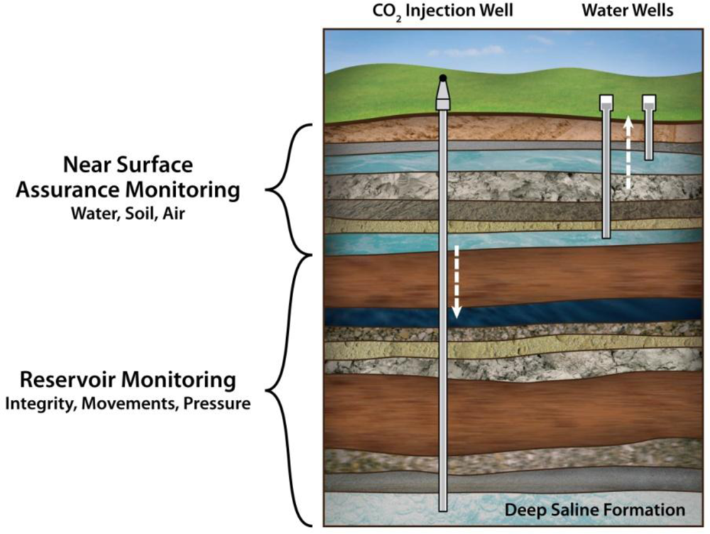
:1. Introduction
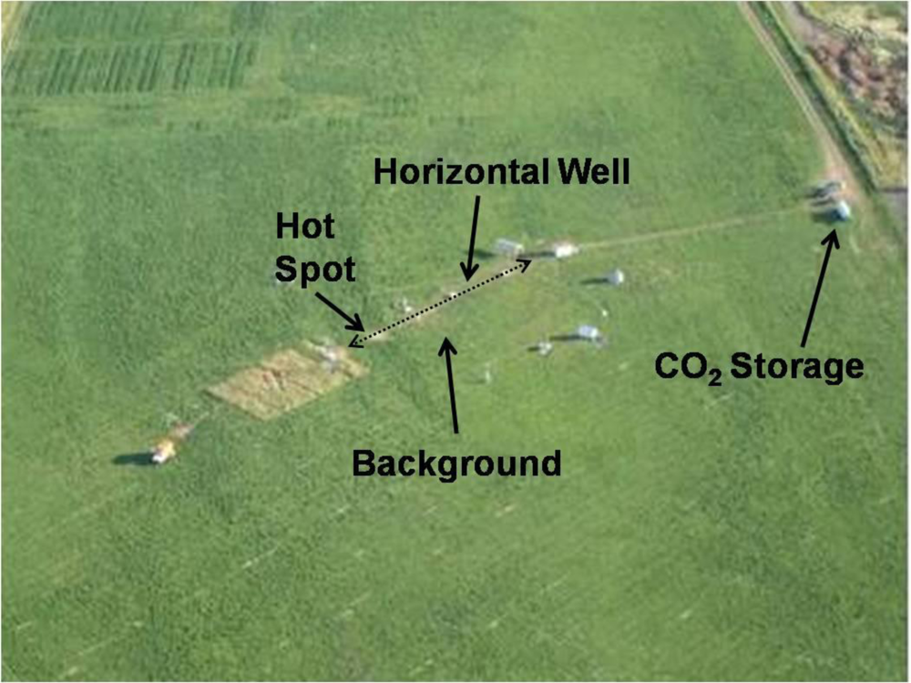
2. Site and Setup
2.1. Site
2.2. INS System
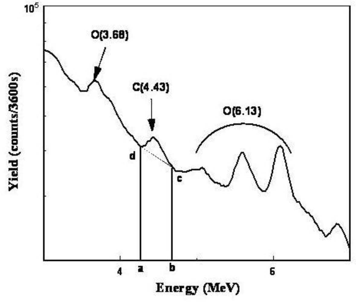
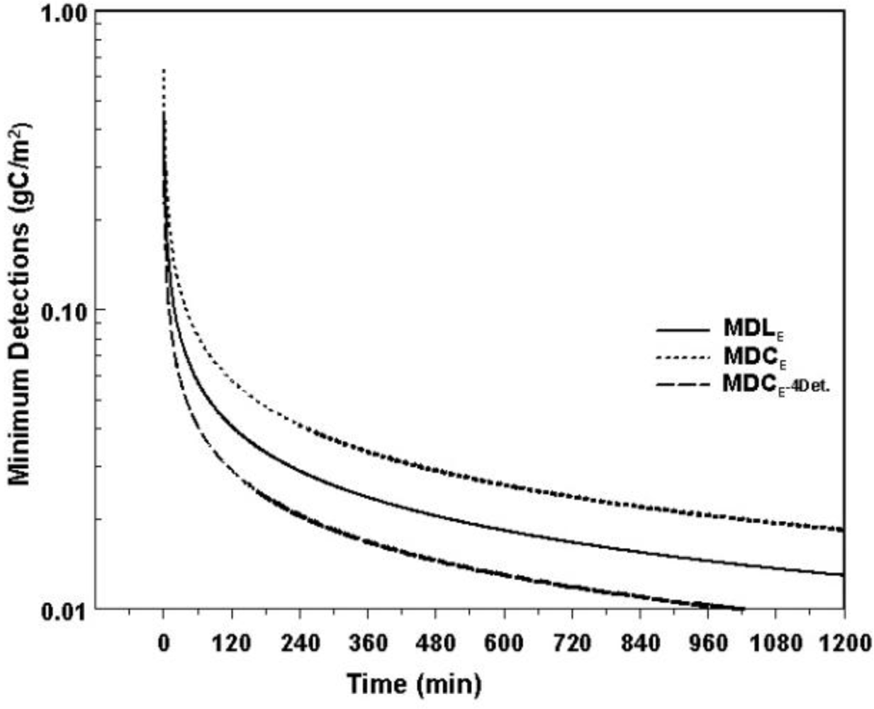
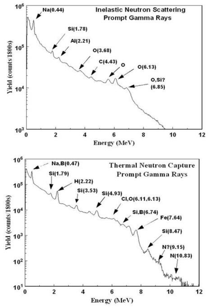
3. Spectral Analysis
4. Results
5. Discussion
6. Summary
Acknowledgments
References
- Tans, P. Trends in Atmospheric Carbon Dioxide—Mauna Loa; US Department of Commerce/National Oceanic and Atmospheric Administration: Boulder, CO, USA. Available online: http://www.esrl.noaa.gov/gmd/ccgg/trends/ (accessed on 9 March 2011).
- International Energy Outlook 2007; Energy Information Administration, US Department of Energy (EIA): Washington, DC, USA, May 2007. Available online: http://www.eia.doe.gov/oiaf/ieo/ (accessed on 9 March 2011). .
- Socolow, R; Hotinski, R; Greenblatt, JB; Pacala, P. Solving the climate problem—Technologies available to curb CO2 emissions. Environment 2004, 46, 8–19. [Google Scholar]
- Greenblatt, JB; Sarmiento, JL. Variability and climate feedback mechanisms in ocean uptake of CO2. In The Global Carbon Cycle: Integrating Humans, Climate, and the Natural World; Field, CB, Raupach, MR, Eds.; Island Press: Washington, DC, USA, 2004. [Google Scholar]
- Carbon Sequestration Technology Roadmap and Program Plan; United States Department of Energy/Office of Fossil Energy/National Energy Technology Laboratory (USDOE/FE/NETL): Pittsburgh, PA, USA, 2007. Available online: http://www.netl.doe.gov (accessed on 9 March 2011).
- Using the Class V Experimental Technology Well Classification for Pilot GS Projects; UIC Program Guidance (UICPG #83); Environmental Protection Agency (EPA): Washington, DC, USA, 2007.
- Core Energy, LLC Class V UIC Injection Permit; Permit No MI-137-5X25-0001; Environmental Protection Agency (EPA): Washington, DC, USA, draft version issued July 2008.
- Underground Injection Control Program (UIC); Environmental Protection Agency (EPA): Washington, DC, USA, 12 February 2008. Available online: http://www.epa.gov/safewater/uic/index.html (accessed on 8 June 2008).
- Geologic Sequestration of Carbon Dioxide; Environmental Protection Agency (EPA): Washington, DC, USA, 2008. Available online: http://www.epa.gov/safewater/uic/wells_sequestration.html (accessed on 9 March 2011).
- International Panel on Climate Change (IPCC). IPCC Special Report on Carbon Doxide Capture and Storage; Metz, B, Davidson, O, de Coninck, H, Loos, M, Meyer, L, Eds.; Cambridge University Press: Cambridge, UK, 2005; p. 195. [Google Scholar]
- Best Practices for: Monitoring, Verification, and Accounting of CO2 Stored in Deep Geologic Formation; DOE/NETL-311/081508; United States Department of Energy/Office of Fossil Energy/National Energy Technology Laboratory (USDOE/FE/NETL): Pittsburgh, PA, USA, 2009.
- Lewicki, JL; Hilley, GE; Laura Dobeck, L; Spangler, L. Dynamics of CO2 fluxes and concentrations during a shallow subsurface CO2 release. Environ. Earth Sci 2010, 60, 285–297. [Google Scholar]
- Saripalli, P; Amonette, J; Rutz, F; Gupta, N. Deign of sensor networks for long term monitoring of geological sequestration. Energy Convers. Manage 2006, 47, 1968–1974. [Google Scholar]
- West, JM; Pearce, JM; Coombs, P; Ford, JR; Scheib, C; Colls, JJ; Smith, KL; Steven, MD. The impact of controlled injection of CO2 on the soil ecosystem and chemistry of an English lowland pasture. Energy Procedia 2009, 1, 1863–1870. [Google Scholar]
- Wielopolski, L; Mitra, S. Near-surface soil carbon detection for monitoring CO2 seepage from a geological reservoir. Environ. Earth Sci 2010, 60, 307–312. [Google Scholar]
- Anderson, DE; Farrar, CD. Eddy covariance measurement of CO2 flux to the atmosphere from the area of high volcanogenic emissions, Mammoth Mountain, California. Chem. Geol 2001, 177, 31–42. [Google Scholar]
- Annunziatellis, A; Beaubien, SE; Bigi, SE; Ciotoli, S; Coltella, G; Lombardi, M. Gas migration along fault systems and through the vadose zone in the Latera caldera (central Italy) implications for CO2 geological storage. Int. J. Greenh. Gas Control 2008, 2, 253–372. [Google Scholar]
- Spangler, LH; Dobeck, LM; Repasky, KS; Nehrir, A; Humphries, S; Barr, J; Keith, C; Shaw, J; Rouse, J; Cunningham, A; et al. A controlled field pilot for testing near surface CO2 detection techniques and transport models. Energy Procedia 2009, 1, 2143–2150. [Google Scholar]
- Spangler, LH; Dobeck, LM; Repasky, KS; Nehrir, AR; Humphries, SD; Barr, JL; Keith, CJ; Shaw, JA; Rouse, JH; Cunningham, AB; et al. A shallow subsurface controlled release facility in Bozeman, Montana, USA, for testing near surface CO2 detection techniques and transport models. Environ. Earth Sci 2010, 60, 227–239. [Google Scholar]
- Wielopolski, L; Hendrey, G; Johnsen, K; Mitra, S; Prior, SA; Rogers, HH; Torber, HA. Nondestructive system for analyzing carbon in the soil. Soil Sci. Soc. Am. J 2008, 72, 1269–1277. [Google Scholar]
- Wielopolski, L; Mitra, S; Hendrey, G; Orion, I; Prior, S; Rogers, H; Runion, B; Torbert, A. Non-destructive Soil Carbon Analyzer (ND-SCA). BNL Report No.72200-2004; Brookhaven National Lab; Upton, NY, USA, 2004. [Google Scholar]
- Wielopolski, L; Johnston, K; Zhang, Y. Comparison of soil analysis methods based on samples withdrawn from different volumes: Correlations versus Calibrations. Soil Sci. Soc. Am. J 2010, 74, 812–819. [Google Scholar]
- Wielopolski, L; Chatterjee, A; Mitra, S; Lal, R. In Situ Determination of Soil Carbon Pool by Inelastic Neutron Scattering: Comparison with Dry Combustion. Geoderma 2010, 160, 394–399. [Google Scholar]
- Evans, RD. The Atomic Nucleus; McGraw-Hill Book Company: New York, NY, USA, 1955; p. 746. [Google Scholar]
- Bevington, FP; Robinson, DK. Data Reduction and Error Analysis for the Physical Sciences; McGraw-Hill Book Company: New York, NY, USA, 1969; p. 56. [Google Scholar]


| 2008—During Injection | ||||||
| Hot Spot (HS) | Background (B) | |||||
| Si | O | C | Si | O | C | |
| N | 8 | 8 | 7 | 12 | 12 | 11 |
| Mean | 1,031,332 | 622,914 | 47,137 | 1,008,545 | 636,929 | 53,704 |
| STD Deviations | 24,858 | 28,328 | 3,610 | 16,530 | 48,235 | 4,731 |
| STD Deviations (%) | 2.4 | 4.5 | 7.4 | 1.6 | 7.5 | 8.8 |
| STD Error (%) | 0.8 | 1.6 | 2.8 | 0.5 | 2.2 | 2.7 |
| Δ (1 − HS/B) × 100 | 2.3 | −2.2 | −14.0 | --- | --- | --- |
| 2009—Pre-Injection | ||||||
| Hot Spot | Background | |||||
| Si | O | C | Si | O | C | |
| N | 9 | 9 | 8 | 5 | 5 | 5 |
| Mean | 787,977 | 650,746 | 79,728 | 759,986 | 665,833 | 81,228 |
| STD Deviations | 15,066 | 13,714 | 4,850 | 5,860 | 5,811 | 3,916 |
| STD Deviations (%) | 1.9 | 2.1 | 6.1 | 0.8 | 0.9 | 4.8 |
| STD Error (%) | 0.6 | 0.7 | 2.2 | 0.4 | 0.4 | 2.1 |
| Δ (1 − HS/B) × 100 | 3.7 | −2.3 | −1.9 | --- | --- | --- |
| 2009—Post-Injection | ||||||
| Hot Spot | Background | |||||
| Si | O | C | Si | O | C | |
| N | 9 | 9 | 8 | 3 | 3 | 3 |
| Mean | 842,562 | 628,521 | 78,850 | 812,448 | 635,948 | 84,718 |
| STD Deviations | 19,889 | 7,117 | 6,079 | 5,751 | 8,725 | 4,566 |
| STD Deviations (%) | 2.4 | 1.1 | 7.6 | 0.7 | 1.4 | 5.4 |
| STD Error (%) | 0.8 | 0.4 | 2.7 | 0.4 | 0.8 | 3.1 |
| Δ (1 − HS/B) × 100 | 3.7 | −1.2 | −6.9 | --- | --- | --- |
| Year | 2008 | 2009 | Combined |
| n | 20 | 27 | 47 |
| Mean | 3,338,759 | 2,102,343 | 3,232,342 |
| SDEV (%) | 43,119 (1.29) | 15,384 (0.73) | 65,455 (2.03) |
| CV (%) | 9,642 (0.29) | 2,961 (0.14) | 9,548 (0.30) |
© 2011 by the authors; licensee MDPI, Basel, Switzerland This article is an open-access article distributed under the terms and conditions of the Creative Commons Attribution license (http://creativecommons.org/licenses/by/3.0/).
Share and Cite
Wielopolski, L. Geological Carbon Sequestration: A New Approach for Near-Surface Assurance Monitoring. Int. J. Environ. Res. Public Health 2011, 8, 818-829. https://doi.org/10.3390/ijerph8030818
Wielopolski L. Geological Carbon Sequestration: A New Approach for Near-Surface Assurance Monitoring. International Journal of Environmental Research and Public Health. 2011; 8(3):818-829. https://doi.org/10.3390/ijerph8030818
Chicago/Turabian StyleWielopolski, Lucian. 2011. "Geological Carbon Sequestration: A New Approach for Near-Surface Assurance Monitoring" International Journal of Environmental Research and Public Health 8, no. 3: 818-829. https://doi.org/10.3390/ijerph8030818
APA StyleWielopolski, L. (2011). Geological Carbon Sequestration: A New Approach for Near-Surface Assurance Monitoring. International Journal of Environmental Research and Public Health, 8(3), 818-829. https://doi.org/10.3390/ijerph8030818